A small Universe
Abstract
Many cosmological models assume or imply that the total size of the universe is very large, perhaps even infinite. Here we argue instead that the universe might be comparatively small, in fact not much larger than the currently observed size. A concrete implementation of this idea is provided by the no-boundary proposal, in combination with a plateau-shaped inflationary potential. In this model, opposing effects of the weighting of the wave function and of the criterion of allowability of the geometries conspire to favour small universes. We point out that a small size of the universe also fits well with swampland conjectures, and we comment on the relation with the dark dimension scenario.
Keywords:
No-boundary proposal , Cosmic inflation , Quantum cosmology1 Introduction
Perhaps the most basic characteristic of our universe is that it is big. When extrapolated to present times, the part of the universe that we see in the cosmic microwave background (CMB) has a size of a little over three times the current Hubble radius [1] (about billion light years), which is half a million times the size of the Milky Way. However, we do not know how large the universe actually is, as we cannot see beyond the limit imposed on us by the CMB. It has been suggested repeatedly that the universe might have a non-trivial topology, which would lead to specific patterns in the CMB if the shortest non-trivial loop fits within the observed last scattering surface (e.g. [2, 3, 4, 5]). Such patterns have been searched for, and no evidence of their existence has been found (e.g. [6, 7, 8, 9, 10, 11, 12, 13, 14]). More subtle correlations might be detectable even if the non-trivial topological feature is larger than the region seen in the CMB, see [15, 16, 17]. In the meantime, we will assume here that the universe possesses a simple topology (see also [18]).
In the absence of observational evidence, we may ask: how large do we expect the universe to be, based on our current understanding of theoretical cosmology? This is the question that concerns us in the present paper. Needless to say, the word current is crucial – cosmology has seen spectacular progress over the last century, accompanied by repeated, significant changes in our outlook on the universe. Also, few complete cosmological models exist. Most models describe only what happens to a certain (comoving) region of the universe, without implications for (or restrictions on) how many such regions might exist in total. But if we want to address the question of the size of the universe, we must do so in a complete cosmological model.
A heuristic view that has been advocated repeatedly is that the universe might have started out at the Planck (energy) scale, with wild fluctuations in geometry and matter configurations. Somewhere, it is argued, the conditions will turn out to be right for inflation to start and the corresponding region of the universe then develops into the large universe we see. However, it is typically not said how this beginning is supposed to have occurred and how many favourable regions one might expect to develop. In some sense, eternal inflation improved upon this scenario by showing that, if it occurs, the late time characteristics of the universe will essentially be independent of the beginning, as we would then be removed from the beginning by a possibly infinite number of tunneling events, in which a new inflating spacetime region of the universe is created from a preexisting inflationary patch of the universe. In this kind of model, the universe is then predicted to be spatially infinite.
This infinity leads to paradoxes, for example with regard to assigning probabilities in quantum theory, as in an infinite universe events that are not forbidden occur infinitely often [19, 20]. In fact the general question of a measure on such a set of pocket universes remains completely unresolved and may well be misguided. Specifying a measure assumes the existence of an overall slicing, which may be seen as an overall time coordinate in this multiverse. If one imagines one, then regions with the same field configurations exist at various ‘times’, and in fact a given set of field configurations is reproduced arbitrarily often globally. This causes the action to diverge [21], which signals a semi-classical inconsistency of the model. For these reasons, we deem eternal inflation to be physically inconsistent.
Another complete cosmological model that has been proposed is that of a cyclic universe, in which the universe is rendered smooth during ekpyrotic contracting phases and in which local quantities evolve cyclically [22]. This model also assumes a spatially infinite universe. Because the smoothing occurs at a low energy scale it avoids the worst issues with assigning a measure [23], though the problem with assigning quantum probabilities remains. For this kind of model, the action is also found to diverge [21], which we again take as a sign of semi-classical inconsistency. Moreover, the physics of the bounce phase remains insufficiently understood.
This leaves us with models of ordinary, non-eternal inflation, which however must be completed in the sense that their beginning must be explained (it is not possible to assume that ordinary inflation was the first phase of evolution of the universe because this leads both to a classical singularity [24] – see [25, 26, 27] for recent developments – and a semi-classical instability [28]). This brings us to the best understood theories of the origin of the universe: the no-boundary [29] and tunnelling proposals [30]. In both of these frameworks spacetime and matter emerge from a quantum tunnelling event out of nothing. The big bang singularity is replaced by a smooth, regular, quantum geometry which includes a Euclidean (or near-Euclidean) region where the big bang would have been. For a cartoon of the idea see Fig. 1, and for a detailed description see [31]. Because these no-boundary field configurations are both compact and regular, the action is automatically finite. Nevertheless, in the case of the tunnelling proposal the wave function favours anisotropic configurations to such an extent that the wave function becomes non-normalisable, and for this reason we will focus on the no-boundary wave function here, for which isotropic universes receive the highest weighting. In this sense a no-boundary origin immediately explains the observed spatial isotropy on the largest scales.

An intriguing feature of the no-boundary wave function is that it leads to the appearance of classical, Lorentzian universes only in the presence of a dynamical attractor [32]. Inflation can play precisely this role. (Ekpyrotic cosmology could too [33, 34, 35].) In fact, only a few -folds of inflationary evolution are required to localise the wave function on Lorentzian histories. However, in order to explain the present-day features of our universe, in particular its spatial flatness, a longer inflationary phase is required. This is because the basic no-boundary requirements of compactness and regularity force the universe to have closed spatial sections (as reviewed in, e.g., [31]). In other words, given our assumption of a trivial spatial topology, on large scales the universe is described by a Robertson-Walker metric with spatial -spheres11 1 Other topologies with closed spatial sections are possible. An example is which has been shown to be suppressed compared to in the no-boundary wave function [36, 37]. We should note that the contribution of more intricate topologies has not been widely explored to date.,
| (1) |
This feature may be at odds with observations, which show that the average curvature is currently very small. It is useful to look at these aspects more quantitatively now.
2 Size of the Universe
The evolution of the universe may be described by the Friedmann equation
| (2) |
with
| (3) |
Here a dot denotes a derivative with respect to the time coordinate , and we have assumed the presence of a scalar field with a potential . We have also included pressure-free matter and radiation, with present-day densities and respectively, which in these models are created at reheating. We are ignoring dark energy, though, since it is negligible for the present discussion. Finally, we are working in units where Newton’s gravitational constant is set to and where the speed of light is set to unity.
Observations show that the curvature term is currently very small, the Planck CMB data alone22 2 There has been stronger evidence for from CMB data alone [38], but when combined with baryonic acoustic oscillations data one recovers consistency with a flat universe at the cost of tension between the datasets – for different views see, e.g., [39, 40, 41, 42, 43, 44]. finding [45]
| (4) |
This is puzzling, as the curvature term has been growing during the phases of radiation () and matter () domination. A standard resolution of this puzzle is to invoke an inflationary phase, during which the curvature term shrinks. For a slow-roll no-boundary history the Lorentzian evolution coincides pretty closely with that of a closed de Sitter universe at constant vacuum energy , with scale factor
| (5) |
where the nucleation scale (which to a first approximation can be thought of as the onset of the classical evolution) is given by
| (6) |
Thus, during the inflationary phase the curvature component is given by
| (7) |
where we defined the number of -folds of inflation as , and where the approximation holds at late times. Importantly, we see that the curvature scales as an exponential of the -folding number during inflation.
Putting the various phases together, we find that at present times we may expect the curvature term to be given by
| (8) |
where the duration of inflation from nucleation to reheating is . Here and denote the temperature and redshift at matter-radiation equality. As one can see, the value of the curvature term depends crucially on the amount of inflation. In fact, we can turn this relation around and find the minimal number of -folds of inflation required to fit the current observational bounds on the curvature. Using , , one finds (see also [46, 45])
| (9) |
This minimal amount depends sensitively on the scale of inflation, which we have assumed coincides with the scale of reheating.
What is the implied current size of the universe in these models? To determine this, we start from the size at nucleation and factor in the subsequent evolutionary phases:
| (10) |
Now . If we assume for the moment that there was a minimal amount of inflation [cf. (2)], then using we see that the current size of the universe becomes independent of the nucleation scale, i.e. independent of the scale of inflation. This happens because a higher inflationary scale implies a smaller nucleation size but also a more pronounced inflationary expansion, and the two effects exactly compensate each other – see Fig. 1 for an illustration. In fact, by assumption, the size comes out as being on the order of the currently observable scale,
| (11) |
Thus, if inflation lasted not much longer than necessary to resolve the flatness puzzle, the size of the universe is just a few times larger than the currently observable size, with a closed spatial geometry.
3 Allowability
But the crucial question is: why would we expect a small number of -folds of inflation? In the no-boundary framework, inflationary histories obtain a probability that depends on the location of the scalar field in the inflationary potential at the onset of the inflationary phase, according to
| (12) |
(Here is the real part of the scalar field at the South Pole of the instanton.) This expression shows that low values of the potential come out as vastly preferred. Typically, this will imply an inflationary phase that is much too short to resolve the flatness puzzle and to generate appropriate cosmological perturbations. However, it has recently been realised that not all no-boundary instantons are likely to make sense in quantum gravity, as some of them develop an instability [47, 48].
No-boundary instantons are generally described by complex instantons. In the context of quantum field theory, Kontsevich & Segal [49] proposed that complex metrics should only be allowed if they lead to convergent path integrals once all possible (-form) matter types have been included. Explicitly, their criterion reads
| (13) |
where is the action and is the -form field strength in dimensions. Pointwise, one can write the metric in diagonal form (no summation), and then the above criterion simplifies to the condition
| (14) |
Roughly speaking, one can say that the metric is allowed to be complex, but not too much.
If one extends this criterion to quantum gravity, as Witten [50] has suggested, then one finds that certain types of metrics are not allowed, precisely because matter path integrals would diverge on such backgrounds. Concretely, one can determine the allowability as follows (for details, see [51, 48]). For the case of interest to us, the metric depends only on (complexified) time. A particular solution may then be represented by a path in the complex time plane – the details of this calculation can be found in A. In the no-boundary case this is a path from the origin (where we choose the South Pole to be located) up to the final point, which represents the late-time hypersurface on which the evolution ends; see Fig. 2. One should now picture two curves, emanating from the origin and saturating the inequality (14), i.e. two lines with and The actual solution is allowable if it lies in between these two extremal lines. It turns out that in the case of interest to us only the maximal line () is important, the other extremal line lying at . If the actual solution lies entirely below that line, the solution is allowed.
This has consequences for no-boundary solutions. As was shown in [50, 52], pure de Sitter instantons are always allowed. However, as discussed in [47, 48], this is no longer true when a scalar field with a potential is added. More specifically, in [48] it was shown that only certain types of potentials (mostly concave potentials) admit allowable no-boundary solutions that lead to -folds of inflationary expansion. The preference for concave/plateau-type potentials may be understood as follows: when the potential is steeper, it requires a more complex scalar field. For instance, at the ‘bottom’ (South Pole) of the no-boundary instanton, to a first approximation the scalar field value is given by
| (15) |
where is the slow-roll parameter. A more complex scalar implies a more complex metric in turn, and this fact then disallows no-boundary instantons starting out on a steep slope of the potential.
In the present paper we do not take the amount of inflation for granted. Rather, we ask: for a given potential, how many -folds of inflation are required in order for the associated no-boundary instantons to be allowed? When the potential is of plateau type, then a longer inflationary phase means starting out on a flatter region of the potential and hence will improve the allowability properties of the associated no-boundary solutions.
4 Example
We can illustrate this with an explicit example, for the family of potentials given by the (natural inflation [53]) form
| (16) |
where is a parameter. Then we find that small amounts of inflation lead to non-allowable instantons and are thus excluded. But above a minimal amount the instanton has sufficiently small complex parts of the metric to be allowed. The specific minimal number of -folds depends on the parameter , as shown in Fig. 3. For example, when we find , while for we find .
If we combine this finding with the preference of no-boundary probabilities for starting out low on the potential, we find that the most likely histories are those that have precisely the minimal number of -folds required for allowability. This situation is sketched in Fig. 4.
We should now see whether these preferred solutions can also be in agreement with observations. Their predictions for the spectral index of density perturbations, as well as the amplitude of gravitational waves (quantified by the tensor-to-scalar ratio ), are shown in Fig. 5, while the predictions for the running of the spectral index are in Fig. 6. Figure 5 shows that the models that are in good agreement with observational data are those with . These models predict a fairly small running, within current observational bounds, but at a level that is detectable by not-too-distant future experiments.
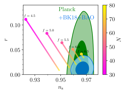

A surprising aspect of this analysis is that a priori we have no idea what might be. It could have turned out to be or (and for some potentials it might very well reach such values), but it turned out to be of for models that are also in close agreement with observations. This is a remarkable feature. But we must also check whether these models actually solve the flatness puzzle. To this end, we must match the scale of the potential (16) with the observed amplitude of density perturbations. At the pivot scale we have [45] , which, given , implies . This in turn implies a high reheating temperature of about and thus requires at least -folds of inflation in order to explain the current large-scale flatness of the universe [cf. (2)]. This is precisely what we obtain for models with Thus there is a kind of positive conspiracy at play, in that larger means more inflation and better agreement with observational data. It is remarkable that models of this kind provide a possible explanation for the otherwise rather arbitrary seeming value of inflationary -folds.
Note that the models predict a number of -folds that is not much larger than the minimal amount required for obtaining a sufficiently flat universe. Thus, they also imply that the size of the universe is not much larger than the current observable size, illustrating the theme of this paper.
We emphasize that similar results are also obtained for other concave potentials that are in agreement with observational constraints on at the confidence level, bearing in mind that the theoretical predictions and the observed central values and error bars may shift when allowing for spatial curvature (e.g. [55, 56, 57, 39, 38, 45, 41]).
Now that we have seen with the example of an explicit model how allowable no-boundary instantons may imply a relatively small size of the universe, let us comment on a few consequences of this idea.
5 Discussion
We will start by asking how large we may expect to be at present times. This depends very sensitively on the number of -folds of inflation. The minimal number was determined precisely such that . However, and thus if inflation lasts only -folds longer than the minimal number, then . This is the lowest value we can theoretically detect, as the primordial density perturbations also induce perturbations on that scale (and it may in fact be difficult to obtain conclusive evidence below [58, 59]). Thus it still seems possible to directly detect whether or not our universe possesses a small size, but only if inflation lasted little more than the minimal required duration.
Conceptually, a small universe seems to fit rather well with the recent advances in string theory and in particular the restrictions on solutions codified in the swampland programme. These suggest that inflation is hard to obtain: the dS conjecture [60, 61, 62, 63] implies that either or must be large. Plateau models (with small and large ) are particularly well suited: if you start higher up the potential, where it is flatter, then instantons will be more real and more allowable, as illustrated with the examples above. If the trans-Planckian censorship conjecture holds [64, 65, 66], then it would imply a very small , and thus also a very low inflationary scale (perhaps as low as ). This would require a very modest number of -folds of inflation, corresponding to a low reheating temperature and thus a smaller required number of -folds in order to resolve flatness and horizon puzzles. Moreover, a small also makes no-boundary geometries almost real [cf. (15)]. Specific predictions however can only be made in the presence of concrete constructions of potentials – we will thus leave this question for future work.
Another consequence of the swampland conjectures is that they must also apply to the current dark energy phase. Then they imply that dark energy must decay. If its potential becomes negative, the universe may even recollapse in a short period of time (see [67] for a study of this scenario). This would then imply a universe that is not only small spatially, but also in temporal extent. This would have the further consequence of rendering the universe rather stable to vacuum decay.
A further idea that has emerged from the swampland programme is that of an additional mesoscopic spatial dimension, called the dark dimension (see, e.g., [68, 69] and references therein). One puzzle with this scenario is how this dimension can be combined with inflation occurring in the other large dimensions, due to the Higuchi bound which effectively implies that there can be no extra internal dimension that is larger than the size of an inflating universe [70]. Here we see a possible resolution: the universe can simply nucleate at a large size already, corresponding to a low inflationary scale, in an isotropic -dimensional configuration. One might then imagine a mechanism by which spatial dimensions inflate, while one dimension is held fixed.
As a concluding thought, let us point out that dark energy currently provides the largest physical scale known. Understanding it will likely require a better understanding of quantum gravity, in perfect illustration of the emerging principle that quantum gravity affects both the smallest and largest scales accessible to us. Here we have seen that quantum cosmology gives us a reason to think that the size of the entire universe may be given by the same scale and may not be more than a few orders of magnitude larger than the currently visible part.
Acknowledgements
JLL thanks Oliver Janssen for explaining the numerical methods used in [48]. JLL gratefully acknowledges the support of the European Research Council via the ERC Consolidator Grant CoG 772295 “Qosmology”. This research was supported in part by the Perimeter Institute for Theoretical Physics. Research at the Perimeter Institute is supported by the Government of Canada through the Department of Innovation, Science and Economic Development and by the Province of Ontario through the Ministry of Colleges and Universities.
Appendix A Allowable complex paths
We consider general relativity minimally coupled to a scalar field with a potential in natural units () and with the cosmological metric
| (17) |
the equations of motion read
| (18a) | ||||
| (18b) | ||||
while the constraint is
| (19) |
No-boundary solutions are then regular solutions satisfying at the South Pole and reaching specified final values , at a final time (see, e.g., [31]). In order to obtain such solutions one must find a suitable (complex) scalar field value at . This works (typically with the use of a numerical optimisation algorithm) as long as the potential is such that it leads to a dynamical attractor, in our case inflation. In the slow-roll case one typically has
| (20) |
while
| (21) |
One may then think of the no-boundary solution as a path in the complex time plane starting at and ending at ; see Fig. 2. Reference [71] provides further details.
We would now like to know whether the solution along this path (let us call it with real parameter ) is allowable or not [51, 48]. For this, we may directly solve the equations of motion along the path. The metric then becomes
| (22) |
where a prime denotes a derivatives with respect to . Note that is generally complex valued. Then using the chain rule () we get the equations of motion along the path,
| (23a) | ||||
| (23b) | ||||
The equation for the maximal allowed curve is [cf. saturating the inequality (14)]
| (24) |
where for the maximal curve we can remove the absolute value signs (the curve always moves up and to the right in the region of interest, and the imaginary part of is positive and small for the solutions of interest compared to the positive real part). Only the argument of is fixed, and a solution with unit modulus is
| (25) |
We can also take a derivative to obtain an expression for ,
| (26) |
which can then be substituted into the equations of motion, ending up with
| (27a) | ||||
| (27b) | ||||
These are the equations that are then solved numerically in order to obtain the results shown in Fig. 3. We find that the level of numerical precision that is required is very high. For instance, we find that for solutions expanding by -folds, we typically need to retain about decimal places in the numerical calculations. As described in the main text, if lies below the maximal curve, then an allowable path can be found. Otherwise we deem the solution unphysical.
References
- [1] J.R. Gott, III, M. Juric, D. Schlegel, F. Hoyle, M. Vogeley, M. Tegmark et al., A map of the universe, Astrophys. J. 624 (2005) 463 [astro-ph/0310571].
- [2] M. Lachièze-Rey and J.P. Luminet, Cosmic topology, Phys. Rept. 254 (1995) 135 [gr-qc/9605010].
- [3] N.J. Cornish, D.N. Spergel and G.D. Starkman, Circles in the sky: Finding topology with the microwave background radiation, Class. Quant. Grav. 15 (1998) 2657 [astro-ph/9801212].
- [4] G.D. Starkman, Topology and cosmology, Class. Quant. Grav. 15 (1998) 2529.
- [5] J.J. Levin, Topology and the cosmic microwave background, Phys. Rept. 365 (2002) 251 [gr-qc/0108043].
- [6] N.J. Cornish, D.N. Spergel, G.D. Starkman and E. Komatsu, Constraining the topology of the universe, Phys. Rev. Lett. 92 (2004) 201302 [astro-ph/0310233].
- [7] J. Shapiro Key, N.J. Cornish, D.N. Spergel and G.D. Starkman, Extending the WMAP Bound on the Size of the Universe, Phys. Rev. D 75 (2007) 084034 [astro-ph/0604616].
- [8] P. Bielewicz and A.J. Banday, Constraints on the topology of the Universe derived from the 7-year WMAP data, Mon. Not. Roy. Astron. Soc. 412 (2011) 2104 [arXiv:1012.3549].
- [9] P.M. Vaudrevange, G.D. Starkman, N.J. Cornish and D.N. Spergel, Constraints on the Topology of the Universe: Extension to General Geometries, Phys. Rev. D 86 (2012) 083526 [arXiv:1206.2939].
- [10] R. Aurich and S. Lustig, A search for cosmic topology in the final WMAP data, Mon. Not. Roy. Astron. Soc. 433 (2013) 2517 [arXiv:1303.4226].
- [11] J.P. Luminet, Cosmic topology: Twenty years after, Grav. Cosmol. 20 (2014) 15 [arXiv:1310.1245].
- [12] Planck collaboration, P.A.R. Ade et al., Planck 2013 results. XXVI. Background geometry and topology of the Universe, Astron. Astrophys. 571 (2014) A26 [arXiv:1303.5086].
- [13] Planck collaboration, P.A.R. Ade et al., Planck 2015 results - XVIII. Background geometry and topology of the Universe, Astron. Astrophys. 594 (2016) A18 [arXiv:1502.01593].
- [14] J.P. Luminet, The Status of Cosmic Topology after Planck Data, Universe 2 (2016) 1 [arXiv:1601.03884].
- [15] COMPACT collaboration, Y. Akrami et al., The Search for the Topology of the Universe Has Just Begun, arXiv:2210.11426.
- [16] COMPACT collaboration, P. Petersen et al., Cosmic topology. Part I. Limits on orientable Euclidean manifolds from circle searches, JCAP 01 (2023) 030 [arXiv:2211.02603].
- [17] COMPACT collaboration, J.R. Eskilt et al., Cosmic topology. Part II. Eigenmodes, correlation matrices, and detectability of orientable Euclidean manifolds, arXiv:2306.17112.
- [18] G.J. Galloway, M.A. Khuri and E. Woolgar, The topology of general cosmological models, Class. Quant. Grav. 39 (2022) 195004 [arXiv:2010.06739].
- [19] A.H. Guth, Eternal inflation and its implications, J. Phys. A 40 (2007) 6811 [hep-th/0702178].
- [20] D.N. Page, The Born Rule Dies, JCAP 07 (2009) 008 [arXiv:0903.4888].
- [21] C. Jonas, J.L. Lehners and J. Quintin, Cosmological consequences of a principle of finite amplitudes, Phys. Rev. D 103 (2021) 103525 [arXiv:2102.05550].
- [22] P.J. Steinhardt and N. Turok, Cosmic evolution in a cyclic universe, Phys. Rev. D 65 (2002) 126003 [hep-th/0111098].
- [23] M.C. Johnson and J.L. Lehners, Cycles in the Multiverse, Phys. Rev. D 85 (2012) 103509 [arXiv:1112.3360].
- [24] A. Borde, A.H. Guth and A. Vilenkin, Inflationary space-times are incomplete in past directions, Phys. Rev. Lett. 90 (2003) 151301 [gr-qc/0110012].
- [25] D. Yoshida and J. Quintin, Maximal extensions and singularities in inflationary spacetimes, Class. Quant. Grav. 35 (2018) 155019 [arXiv:1803.07085].
- [26] J.E. Lesnefsky, D.A. Easson and P.C.W. Davies, Past-completeness of inflationary spacetimes, Phys. Rev. D 107 (2023) 044024 [arXiv:2207.00955].
- [27] G. Geshnizjani, E. Ling and J. Quintin, On the initial singularity and extendibility of flat quasi-de Sitter spacetimes, JHEP 10 (2023) 182 [arXiv:2305.01676].
- [28] A. Di Tucci, J. Feldbrugge, J.L. Lehners and N. Turok, Quantum Incompleteness of Inflation, Phys. Rev. D 100 (2019) 063517 [arXiv:1906.09007].
- [29] J.B. Hartle and S.W. Hawking, Wave Function of the Universe, Phys. Rev. D 28 (1983) 2960.
- [30] A. Vilenkin, The Birth of Inflationary Universes, Phys. Rev. D 27 (1983) 2848.
- [31] J.L. Lehners, Review of the no-boundary wave function, Phys. Rept. 1022 (2023) 1 [arXiv:2303.08802].
- [32] J.B. Hartle, S.W. Hawking and T. Hertog, The Classical Universes of the No-Boundary Quantum State, Phys. Rev. D 77 (2008) 123537 [arXiv:0803.1663].
- [33] L. Battarra and J.L. Lehners, On the Creation of the Universe via Ekpyrotic Instantons, Phys. Lett. B 742 (2015) 167 [arXiv:1406.5896].
- [34] L. Battarra and J.L. Lehners, On the No-Boundary Proposal for Ekpyrotic and Cyclic Cosmologies, JCAP 12 (2014) 023 [arXiv:1407.4814].
- [35] J.L. Lehners, New Ekpyrotic Quantum Cosmology, Phys. Lett. B 750 (2015) 242 [arXiv:1504.02467].
- [36] J.J. Halliwell and J. Louko, Steepest Descent Contours in the Path Integral Approach to Quantum Cosmology. 3. A General Method With Applications to Anisotropic Minisuperspace Models, Phys. Rev. D 42 (1990) 3997.
- [37] R. Bousso and S.W. Hawking, The Probability for primordial black holes, Phys. Rev. D 52 (1995) 5659 [gr-qc/9506047].
- [38] Planck collaboration, N. Aghanim et al., Planck 2018 results. VI. Cosmological parameters, Astron. Astrophys. 641 (2020) A6 [arXiv:1807.06209].
- [39] C.G. Park and B. Ratra, Using the tilted flat-CDM and the untilted non-flat CDM inflation models to measure cosmological parameters from a compilation of observational data, Astrophys. J. 882 (2019) 158 [arXiv:1801.00213].
- [40] E. Di Valentino, A. Melchiorri and J. Silk, Planck evidence for a closed Universe and a possible crisis for cosmology, Nature Astron. 4 (2019) 196 [arXiv:1911.02087].
- [41] W. Handley, Curvature tension: evidence for a closed universe, Phys. Rev. D 103 (2021) L041301 [arXiv:1908.09139].
- [42] G. Efstathiou and S. Gratton, The evidence for a spatially flat Universe, Mon. Not. Roy. Astron. Soc. 496 (2020) L91 [arXiv:2002.06892].
- [43] S. Vagnozzi, A. Loeb and M. Moresco, Eppur è piatto? The Cosmic Chronometers Take on Spatial Curvature and Cosmic Concordance, Astrophys. J. 908 (2021) 84 [arXiv:2011.11645].
- [44] S. Vagnozzi, E. Di Valentino, S. Gariazzo, A. Melchiorri, O. Mena and J. Silk, The galaxy power spectrum take on spatial curvature and cosmic concordance, Phys. Dark Univ. 33 (2021) 100851 [arXiv:2010.02230].
- [45] Planck collaboration, Y. Akrami et al., Planck 2018 results. X. Constraints on inflation, Astron. Astrophys. 641 (2020) A10 [arXiv:1807.06211].
- [46] WMAP collaboration, E. Komatsu et al., Five-Year Wilkinson Microwave Anisotropy Probe (WMAP) Observations: Cosmological Interpretation, Astrophys. J. Suppl. 180 (2009) 330 [arXiv:0803.0547].
- [47] J.L. Lehners, Allowable complex scalars from Kaluza-Klein compactifications and metric rescalings, Phys. Rev. D 107 (2023) 046004 [arXiv:2209.14669].
- [48] T. Hertog, O. Janssen and J. Karlsson, Kontsevich-Segal Criterion in the No-Boundary State Constrains Inflation, Phys. Rev. Lett. 131 (2023) 191501 [arXiv:2305.15440].
- [49] M. Kontsevich and G. Segal, Wick Rotation and the Positivity of Energy in Quantum Field Theory, Quart. J. Math. Oxford Ser. 72 (2021) 673 [arXiv:2105.10161].
- [50] E. Witten, A Note On Complex Spacetime Metrics, arXiv:2111.06514.
- [51] C. Jonas, J.L. Lehners and J. Quintin, Uses of complex metrics in cosmology, JHEP 08 (2022) 284 [arXiv:2205.15332].
- [52] J.L. Lehners, Allowable complex metrics in minisuperspace quantum cosmology, Phys. Rev. D 105 (2022) 026022 [arXiv:2111.07816].
- [53] K. Freese, J.A. Frieman and A.V. Olinto, Natural inflation with pseudo-Nambu-Goldstone bosons, Phys. Rev. Lett. 65 (1990) 3233.
- [54] BICEP, Keck collaboration, P.A.R. Ade et al., Improved Constraints on Primordial Gravitational Waves using Planck, WMAP, and BICEP/Keck Observations through the 2018 Observing Season, Phys. Rev. Lett. 127 (2021) 151301 [arXiv:2110.00483].
- [55] W. Handley, Primordial power spectra for curved inflating universes, Phys. Rev. D 100 (2019) 123517 [arXiv:1907.08524].
- [56] L.T. Hergt, F.J. Agocs, W.J. Handley, M.P. Hobson and A.N. Lasenby, Finite inflation in curved space, Phys. Rev. D 106 (2022) 063529 [arXiv:2205.07374].
- [57] M.I. Letey, Z. Shumaylov, F.J. Agocs, W.J. Handley, M.P. Hobson and A.N. Lasenby, Quantum Initial Conditions for Curved Inflating Universes, arXiv:2211.17248.
- [58] M. Vardanyan, R. Trotta and J. Silk, How flat can you get? A model comparison perspective on the curvature of the Universe, Mon. Not. Roy. Astron. Soc. 397 (2009) 431 [arXiv:0901.3354].
- [59] C.D. Leonard, P. Bull and R. Allison, Spatial curvature endgame: Reaching the limit of curvature determination, Phys. Rev. D 94 (2016) 023502 [arXiv:1604.01410].
- [60] G. Obied, H. Ooguri, L. Spodyneiko and C. Vafa, De Sitter Space and the Swampland, arXiv:1806.08362.
- [61] S.K. Garg and C. Krishnan, Bounds on Slow Roll and the de Sitter Swampland, JHEP 11 (2019) 075 [arXiv:1807.05193].
- [62] H. Ooguri, E. Palti, G. Shiu and C. Vafa, Distance and de Sitter Conjectures on the Swampland, Phys. Lett. B 788 (2019) 180 [arXiv:1810.05506].
- [63] J.L. Lehners, Small-Field and Scale-Free: Inflation and Ekpyrosis at their Extremes, JCAP 11 (2018) 001 [arXiv:1807.05240].
- [64] A. Bedroya and C. Vafa, Trans-Planckian Censorship and the Swampland, JHEP 09 (2020) 123 [arXiv:1909.11063].
- [65] A. Bedroya, R. Brandenberger, M. Loverde and C. Vafa, Trans-Planckian Censorship and Inflationary Cosmology, Phys. Rev. D 101 (2020) 103502 [arXiv:1909.11106].
- [66] K. Kadota, C.S. Shin, T. Terada and G. Tumurtushaa, Trans-Planckian censorship and single-field inflaton potential, JCAP 01 (2020) 008 [arXiv:1910.09460].
- [67] C. Andrei, A. Ijjas and P.J. Steinhardt, Rapidly descending dark energy and the end of cosmic expansion, Proc. Nat. Acad. Sci. 119 (2022) e2200539119 [arXiv:2201.07704].
- [68] M. Montero, C. Vafa and I. Valenzuela, The dark dimension and the Swampland, JHEP 02 (2023) 022 [arXiv:2205.12293].
- [69] L.A. Anchordoqui, I. Antoniadis and D. Lüst, Aspects of the dark dimension in cosmology, Phys. Rev. D 107 (2023) 083530 [arXiv:2212.08527].
- [70] A. Higuchi, Forbidden Mass Range for Spin-2 Field Theory in De Sitter Space-time, Nucl. Phys. B 282 (1987) 397.
- [71] O. Janssen, Slow-roll approximation in quantum cosmology, Class. Quant. Grav. 38 (2021) 095003 [arXiv:2009.06282].
