Learning to Recharge: UAV Coverage Path Planning through Deep Reinforcement Learning
Abstract
Coverage path planning (CPP) is a critical problem in robotics, where the goal is to find an efficient path that covers every point in an area of interest. This work addresses the power-constrained CPP problem with recharge for battery-limited unmanned aerial vehicles (UAVs). In this problem, a notable challenge emerges from integrating recharge journeys into the overall coverage strategy, highlighting the intricate task of making strategic, long-term decisions. We propose a novel proximal policy optimization (PPO)-based deep reinforcement learning (DRL) approach with map-based observations, utilizing action masking and discount factor scheduling to optimize coverage trajectories over the entire mission horizon. We further provide the agent with a position history to handle emergent state loops caused by the recharge capability. Our approach outperforms a baseline heuristic, generalizes to different target zones and maps, with limited generalization to unseen maps. We offer valuable insights into DRL algorithm design for long-horizon problems and provide a publicly available software framework for the CPP problem.
I Introduction
Determining a path that covers every point in an area of interest is the designated goal of the coverage path planning (CPP) problem. Typically, this path should be as short and efficient as possible, making the problem related to the traveling salesman problem [1]. At the same time, other constraints, e.g., collision avoidance, need to be satisfied. When a complete geometric description of the area of interest is available, the CPP problem is proven to be NP-hard [2]. Rapid innovation has enabled unmanned aerial vehicles (UAVs), or drones as they are commonly called, to be used for a wide range of applications that constitute some form of the CPP problem, e.g., smart farming, photogrammetry, disaster management, environmental monitoring, or infrastructure inspection [3]. Including but not limited to these applications, the overall UAV services market is projected to reach a value of USD 189.4 billion by 2030 [4]. When using autonomous quadcopter-type UAVs for the CPP problem, a central constraint is the limited onboard battery capacity that may make repeated recharge cycles necessary to complete a coverage mission.
As a long-standing problem in robotics, numerous path planning algorithms have been proposed to solve various instances of the CPP problem. Most classically, these approaches are either characterized as complete approaches or heuristics [1, 5]. Complete approaches guarantee complete coverage of all free space in the scenario, but may be computationally infeasible, while heuristics do not offer guarantees but are usually computationally simpler. Algorithms of both categories are often based on cellular decomposition of the environment, i.e., a geometric partition into cells that either need to be covered or are seen as obstacles. Each cell is then covered by some strategy, e.g., simple back-and-forth motions, while the order in which the cells are visited is decided by some planning algorithm. Previous works have suggested the use of graph search [6], dynamic programming [7], meta-heuristics [8], or evolutionary algorithms [9] to plan coverage paths for UAVs.
In this work, we formulate the power-constrained CPP problem with recharge. In contrast to most existing problem formulations, we consider an energy-limited case in which a UAV can achieve full coverage of the target region only by carrying out multiple flights with intermediate charging stops. We only consider a coverage mission completed when full coverage of the target region is achieved. Furthermore, we investigate a more generalized form of the CPP problem, where only a subset of the free space is considered a coverage target. This challenging scenario requires optimization over the entire time horizon of the mission, with a complex interplay between flight segments to and from landing zones.
We propose to address this problem using deep reinforcement learning (DRL), as it has the potential to find close to optimal solutions for this NP-hard problem. To that end, we formulate the problem such that the proximal policy optimization (PPO)-based [10] deep reinforcement learning (DRL) agent observes the problem as global and local maps [11] and learns to minimize the steps required to solve the problem. We utilize action masking based on a safety model, which guarantees safety and significantly improves the learning performance of the agent. We address the long-horizon problem by scheduling the discount factor, which balances the importance of immediate and future rewards in the objective. The scheduling allows the agent to first learn to solve the task, followed by continuous improvement on the efficiency of the trajectory. Furthermore, we provide the agent with a history of its positions to aid it in solving an emergent state loop problem that is caused by the recharge capability and the consequential possibility of recreating previously visited states. In the results, we conduct ablation studies on action masking, discount factor scheduling, and position history. Additionally, we highlight the agent’s zero-shot generalization ability, denoting its capacity to solve unseen scenarios without additional training. We evaluate this generalization across various target zones and maps, including its capability to solve unseen maps. As existing approaches from the literature can usually not be easily adapted to the power-constrained CPP problem with recharge, we further provide a model-based greedy heuristic and compare it to our proposed algorithm, showcasing that our DRL approach can reliably find shorter paths to solve the CPP problem.
CPP is a fundamental problem with broad applications, holding the potential to address numerous existing challenges across various domains. However, only a few papers investigated DRL-based methods specifically tailored to the complexities of the UAV coverage problem [11, 12, 13], or investigated the general applicability of DRL for ground-based CPP [14, 15, 16, 17, 18, 19, 20]. In this work, we present several contributions to address these gaps:
- •
We tackle the power-constrained CPP problem with recharge, a critical aspect for battery-limited UAVs operating in large and complex environments, utilizing a PPO-based global-local DRL approach.
- •
Using model-based action masking, we ensure the safety of the generated flight paths.
- •
Through extensive evaluations, we show that our approach outperforms a baseline heuristic, can generalize planning over multiple maps with different characteristics, and can even solve a previously unseen map.
- •
We offer valuable design insights for developing DRL algorithms and corresponding neural network models for long-horizon problems.
- •
Finally, we provide a publicly available software framework11 1 https://github.com/theilem/uavSim.git based on the commonly used OpenAI gym API [21] and include all trained models shown in this work, filling the current gap in available software tools.
This paper is organized as follows: Section II provides an overview of relevant literature in coverage path planning and DRL approaches. In Section III, we introduce the full CPP problem with recharge and associated environmental constraints. Starting from the problem description as a partially observable Markov decision process (POMDP), we introduce our DRL-based solution methodology in Section IV. Section V, which describes our evaluation setup, is followed by a detailed analysis of results and ablation studies in Section VI. We conclude the paper with a summary and an outlook to future work in Section VII.
II Related Work
As CPP is a long-standing problem in robotics, a wide array of solution methods has been proposed. The most classical introduction to the CPP problem and traditional solution methods can be found in [1]. Cabreira et al. [3] provide a survey focusing specifically on decomposition-based CPP approaches for UAVs. In contrast, Tan et al. [22] review existing CPP approaches (not specifically for UAVs) ranging from decomposition-based, exact algorithms to fully random heuristics, including recent deep learning-based approaches.
Focusing on designing coverage paths for UAVs specifically, most previous works suggest non-DRL approaches. An example of planning a coverage path for a UAV through a combination of a genetic algorithm and the rapidly exploring random tree (RRT) method is given in [9], which leads to an optimal path for the specific scenario but is only practical for small maps and simple environments. In [7], the authors suggest solving the underlying traveling salesman problem of flying from one region of interest to the next with dynamic programming and using a straightforward back-and-forth motion to cover the individual regions. They focus on an environment without obstacles and the necessity to recharge. Meta-heuristics like harmony search in [8], specifically for a UAV application scenario in precision agriculture, offer relatively low computation time but without optimality guarantees. Various variants of posing a CPP problem in a graph structure by decomposition and solving it by graph search algorithms have also been suggested. In [6], such an algorithm is developed and evaluated on a real-world UAV system. None of these approaches would be directly applicable to the scenario we investigate, be it for lack of recharging, lower complexity environments, or the scale of the specific CPP scenario.
DRL-based approaches can tackle CPP problems directly and without the need for previous decomposition but are generally underexplored in the context of autonomous UAV coverage missions. One of the rare examples is given in [13], where a Q-learning-based algorithm is proposed for coordinating multiple UAVs on a coverage mission. In contrast to the scenario we investigate, the coverage mission is set in an environment not requiring obstacle avoidance or recharge. It is not based on directly using a map as input to the DRL agent. Our previous work [12, 11], which focuses on generalizing learning over scenario parameters and map-processing techniques is related to this work, but only tackles the CPP problem without recharge.
Considering general CPP approaches for ground-based robots, several works utilize some form of DRL in their solution. In [14], the authors develop an abstraction model for CPP scenarios to find a specific coverage path solution with DRL. In [17], a CPP problem is reformulated as an optimal time-stopping problem, and the authors demonstrate a solution to this problem with a deep Q-network approach for indoor environments. Kyaw et al. [15] use a classical cellular decomposition approach to repose the CPP problem as a traveling salesman problem, then solve it with the help of the REINFORCE algorithm. A more practical perspective is given in [19], where a CPP problem for specific tetromino-shaped reconfigurable robots is solved with the help of an actor-critic type DRL algorithm and compared to various other existing CPP algorithms. In the context of a medical surface disinfecting robot, a graph-based environment representation is used in [20] to solve a CPP problem using a deep Q-network DRL approach. In [16], the authors investigate another form of the CPP problem in unknown environments and also use a map-based DRL approach, but with the combination of local sensory inputs of the robotic platform. All mentioned approaches focus on a scenario where the complete free space is the coverage target, and no recharging is needed. Several other tasks, for which DRL-based solutions were suggested, are closely CPP-related. Typical examples are patrolling [23, 24], which is the task of checking an area of interest repeatedly, and the exploration of unknown environments [25, 26, 27].
With safety being a top concern in path planning for autonomous UAVs, we propose using model-based action masking to constrain the actions available to the DRL agent to a safe subset. Regarding safe learning approaches in RL, this can be classified as a straightforward certifying learning-based control approach [28]. Action masking has been suggested in other domains, e.g., in autonomous driving scenarios [29] or for the vehicle routing problem [30]. Independently of a specific application, the authors in [31] investigate the consequences of using action masking in policy gradient DRL algorithms, while general action space shaping is investigated in [32].
III Problem Formulation
| Description | |
|---|---|
 |
Low/High buildings |
 |
Landing zone |
 |
No-fly zone (NFZ) |
 |
Target zone |
 |
Target + NFZ/Landing |
 |
Cells not covered |
 |
Agent with battery |
 |
Field of view (FoV) |
 |
Trajectory |
 |
Take-off/Charging point |
This section describes the CPP problem by first introducing the UAV grid-world model followed by the CPP objective. Figure 1 visualizes the problem in an example state.
III-A UAV Grid-World
We consider a square grid-world of size with cell width and height where the set of all cell indices is given by . Each cell in the grid-world can be a low or high obstacle, a landing zone, a no-fly zone (NFZ), or empty. The grid-world can thus be described through three Boolean matrices , where the matrices indicate the presence of an obstacle, a landing zone, and NFZ in each cell, respectively. A low obstacle that can be flown over is only defined as an obstacle, while a high obstacle that cannot be passed over is also defined as an NFZ. Landing zones can neither be obstacles nor NFZs. To reduce the use of indexing in the following descriptions, we define the set of obstacles, landing zones, and NFZs as , , and , which contain the indices of all cells for which the respective Boolean matrices are true.
The UAV is assumed to occupy one cell at a time described through its position . It is either flying at cruise altitude or landed at altitude 0, indicated through its landed state , which is true if the UAV is landed and false if it is flying. The UAV has a battery with a known charge, which is defined through the remaining flying time , indicating the number of steps that can be taken until the battery is empty.
The UAV can move to adjacent cells, take off, land, or charge, which is described through an action where
| (1) |
The position of the UAV evolves according to
| (2) |
where is the motion lookup table defined as
| (3) |
The landed state evolves according to
| (4) |
The battery state follows
| (5) |
with being a constant charge amount, and as the maximum capacity of the battery.
The constraints of the UAV grid-world problem are defined through action and state constraints. Action constraints are given as
| (6) | ||||
The UAV can only take off if landed, can only charge if landed and the battery is not full, can only move if flying, and can only land if currently flying and in a landing zone. Constraints on the state are summarized as
| (7a) | ||||
| (7b) | ||||
which define that the UAV cannot be in an NFZ, and the battery cannot be empty unless landed.
III-B Coverage Path Planning
The CPP problem extends the UAV grid-world problem by defining target zones summarized through , with being the set of indices of cells defined as targets. The target evolves according to
| (8) |
in which indicates whether cell is visible from the next position given the obstacles . It thus defines the current field of view (FoV) of the UAV. The initial state of the system is set as
| (9a) | ||||
| (9b) | ||||
with . The initial coverage target consists of multiple random patches with , i.e., no target zones in cells occupied by obstacles. However, target zones can be in NFZs, which need to be covered by flying adjacent to the cells. The initial landing state depends on the objective. We formulate two objectives for the CPP problem.
III-B1 Power-constrained CPP without recharge
In the power-constrained CPP problem without recharge the initial landing state of the UAV is and the objective is
| (10) | ||||
in which
| (11) |
The objective is to minimize the remaining target zone until the agent lands for the first time, while adhering to the action and state constraints, with the initial state flying over a landing zone with a randomized battery level. This objective was used in previous work [12, 11].
III-B2 Power-constrained CPP with recharge
In the power-constrained CPP problem with recharge the initial landing state is and the objective is
| (12) | ||||
The objective is to minimize the number of steps until the remaining coverage target is empty and the UAV is landed, while adhering to the action and state constraints, with the initial state landed in a landing zone with a randomized battery level. This objective is closer to a realistic UAV CPP scenario, but also much more challenging than the previous one as it extends over a significantly longer time-horizon. Therefore, this paper focuses on solving this power-constrained CPP problem with recharge.
IV Methodology
We solve the described problem using reinforcement learning (RL) with model-based action masking for constraint satisfaction. To solve the problem with RL, it needs to be formulated as a Markov decision process (MDP). Since we utilize specific observation functions, we describe the problem as a partially observable Markov decision process (POMDP), which is defined by the tuple . It contains the set of possible states , the set of possible actions , the reward function , and the deterministic state transition function . Furthermore, an observation space describes the agent’s observations, and the observation function defines the mapping from states to observations. The discount factor balances the importance of immediate and future rewards. The state space of the system can be described through
| (13) |
In principle, the discrete action space is as given in (1). However, we mask out infeasible actions based on a safety model.
IV-A Action Masking through Safety Modeling
We consider three different levels of action space restrictions: valid, immediate, and invariant. The valid action mask is defined based on actions that violate the action constraints in (6). These actions are considered invalid as their outcomes are undefined, such as taking off if already flying or trying to fly east while landed. It can be defined as:
| (14) |
with . The valid action mask is the most commonly used in the literature [32].
The immediate action mask disallows actions leading to an immediate next state that violates any constraint, i.e., an action after which the UAV is in an NFZ. Based on the constraints (6) and (7a), it can be defined as:
| (15) |
Finally, the invariant action mask is intended to disallow actions that lead to unrecoverable states. In the grid-world, a state is unrecoverable if the battery level is insufficient to return to a landing zone and recharge, i.e., state constraint (7b). The invariant action mask can be defined by first computing the distance from the nearest landing zone for each cell, using the distance matrix defined recursively as:
| (16) |
The recursion stops at landing zones and NFZs, setting the distance to 1 and , respectively. Using the function that indexes , the state-dependent invariant action space can then be defined as:
| (17) |
All immediately safe actions that lead to a state that is at maximum steps away from a landing zone are invariantly safe. The mask is applied by setting the infeasible action logits of the actor to , which is further described in Section IV-E. Section VI-A ablates the usage of different mask levels.
IV-B Reward Function and Discount Factor
The ideal reward function that reflects the objective in (12) only contains a penalty for each step taken in the environment since, with invariant action masking, the episode only terminates when the remaining coverage target is empty and the agent is landed. However, since the agent learns from scratch, it is highly unlikely, effectively impossible, to solve the problem randomly to observe the termination condition even once. Therefore, some reward shaping is necessary such that the agent is guided toward solving the problem first and then minimizing the number of required steps. We chose to give a reward for every covered cell at the moment of coverage, leading to the following reward function:
| (18) |
With a discount factor , this reward function still yields a return , which is maximized only by decreasing . However, as before, the agent initially does not know how to solve the problem and, thus, the value estimate would be unstable, potentially tending towards depending if or dominates the estimate. On the other hand, a discount factor often results in greedy behavior as early coverage becomes more important than finishing the coverage mission overall faster. To avoid this conundrum, we start with a lower discount factor allowing the agent to learn how to successfully complete the mission and for the value estimate to stabilize. Throughout training, we gradually increase the discount factor , specifically we use
| (19) |
with the starting value , decay rate , decay steps , and the current interaction step .
The suggested discount factor scheduling proves advantageous within finite-horizon problems where the horizon is contingent on the agent’s performance, initially creating the illusion of an infinite problem. This approach stabilizes initial value estimates while facilitating long-horizon optimization during the advanced phases of training. Section VI-B ablates different discount factor scheduling parameters.
IV-C Position History


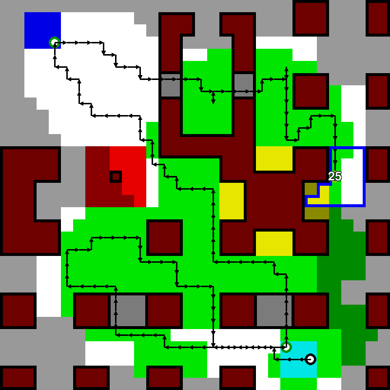
An added challenge through the recharge ability is that the agent can recreate the same state. If the agent takes off, flies around without covering any new target, and then returns to the same landing zone cell to recharge, the same state will be observed after charging. If the actions chosen by the agent are deterministic, the agent will be stuck in this loop, indefinitely. Figure 2 shows two examples of this behavior.
For the agent to avoid getting stuck in such a loop, it either needs to act stochastically or the associated observation needs to change between loops. To alter the observation and help the agent to learn to avoid repeating the same behavior, we augment the state with a position history layer , which evolves according to
| (20) |
with being 1 at and 0 otherwise. All values except the current position in the position history decay with . The position history is concatenated with the other map layers in the observation. Note that we do not add any reward shaping to avoid the revisitation of cells. Section VI-C ablates the usage of the position history.
IV-D Global-Local Observation
We use the global-local observation method from previous work [11] as the observation function. In this method, the agent observes the environment as two maps centered around the agent, a global compressed map and a local full-resolution map. Centering the map was shown to be essential for generalization capabilities in [33]. The motivation for using the global-local observation function is that it outperformed centered observations in [11] and in initial experiments for this paper. The global-local preprocessing appears to aid the agent significantly, and additionally it greatly reduces memory requirements for storing experiences compared to the centered map.
The observation processing pipeline is visualized on the left side of Figure 3. It starts by centering the map around the agent’s position and padding it with obstacles and NFZs, increasing the size to . The global map downsamples the centered map by the global map scaling factor , and the local map crops out an central region, with the local map size . The resulting observation space , is given as
containing the global map the local map and the state scalars, consisting of the normalized battery and the landed state . The layers of the maps are landing zones, NFZs, obstacles, remaining targets, and position history. For simplicity, all channels and scalars are cast to real values.
IV-E Neural Network Architecture

We train the agents using the proximal policy optimization (PPO) algorithm [10]. PPO is a popular and effective reinforcement learning method widely used in various applications. It is an on-policy actor-critic algorithm. In our work, the parameters of the actor and critic, and , parameterize two neural networks with the same structure, shown in Figure 3. After creating the global and local maps, they are embedded by a linear convolution layer into 32 channels. After that, both maps are processed similarly with two convolution layers with ReLU activation function, where the second layer doubles the number of channels, followed by a max pooling. This is repeated three more times, after which the spatial dimensions are reduced by a last max pooling, yielding two 512-element vectors. These vectors are concatenated with the state scalars input and processed through three hidden layers of size 256 and with ReLU activation function. The output layer has no activation function and is a single neuron for the critic and neurons for the actor. At this point, action masking can be applied by setting the output values of the actor to for all infeasible actions. The policy is a of the masked output values.
V Evaluation Setup
V-A Heuristic for Comparison
As the methods described in the literature are not directly applicable to the scenario in this paper, we developed a model-based greedy heuristic as a baseline for comparison. The heuristic determines the nearest reachable cell from which a coverage target cell is visible and flies towards it. If no reachable cell exists, it lands to recharge fully. Algorithm 1 provides a pseudocode of the heuristic. It uses the distance functions that gives the distance in steps from one cell to another, and that provides the distance of a given cell to the closest landing zone. Lines 1-3 state that whenever the agent is landed, it should fully recharge and then take off. If there is no remaining target zone, the agent should fly to the nearest landing zone and land to complete the task (lines 4-7). Otherwise, line 8 computes all cells of interest that are not NFZs and from which a target cell is in FoV. Using these, line 9 determines all reachable cells of interest where the agent could fly and return to a landing zone within its battery constraint. If there is no reachable cell of interest, lines 10-14 compute all reachable landing zones to select the one closest to a cell of interest to fly there and land. This step is essential if the nearest cell of interest is more than a full charge away. If a reachable cell of interest exists, the agent should select the closest and fly toward it (lines 15-16).
return Fly to and land end if 4
if is empty then 5
return Fly to and land end if 6
return Fly to
In the experiments, the heuristic is used to give a baseline against which the performance of the learned agents is measured. We use the relative percentage deviation (RPD) measure to evaluate the performance in the required steps to solve the CPP problem. It is computed as
| (21) |
with and being the steps needed to solve the problem by the agent and heuristic, respectively.
V-B Agents and Maps
For this paper we created 12 maps, shown in Figure 4, with sizes ranging from to . The Manhattan map is used for illustration purposes, as it is small enough but still contains all possible CPP challenges. In the evaluation, we focus on the Suburban, Castle, TUM, Cal, and Border maps. As target zones can also be within NFZs, the Suburban map has the specific challenge that the agent might need to pass on both sides of the wide NFZs to cover target zones. The Castle map is challenging because of the long distances traveled to access points on the map. The castle-like shape on the top left that surrounds a landing zone further complicates the path planning. The specific challenge of the TUM map is that the agent needs to learn the difference between low and high obstacles to fly into the inner area of the bottom left region. No specific added challenges are present in the Cal map, but it contains irregular low and high buildings. Finally, the Border map is dominated by a barrier-like obstacle that divides the task area in the middle and can only be circumvented near the edges of the map. The Cal and Border maps are used for our zero-shot out-of-distribution generalization experiments to evaluate how the agent can solve simple and complicated maps that it did not encounter before.
We trained multiple agents on different subsets of maps, shown in Table I. The Multi agents are trained on multiple maps, where in each training episode, a map is chosen uniformly at random. The other agents are trained only on one map, and are referred to as specialized agents. Unless stated otherwise, all agents are trained using the parameters in Table II. For each configuration, three agents were trained. Each training procedure ran for around four days on an NVIDIA A100 GPU.
|
Manhattan |
Manhattan2 |
Town |
City |
Open |
Urban |
Urban2 |
Suburban |
Castle |
TUM |
Cal |
Border | |
| Size | 32 | 32 | 32 | 40 | 44 | 50 | 50 | 38 | 50 | 50 | 42 | 50 |
| T/O | 1000 | 1000 | 1000 | 1200 | 1300 | 1500 | 1500 | 1200 | 1500 | 1500 | 1300 | 1500 |
| Multi10 | ✓ | ✓ | ✓ | ✓ | ✓ | ✓ | ✓ | ✓ | ✓ | ✓ | ✗ | ✗ |
| Multi3 | ✗ | ✗ | ✗ | ✗ | ✗ | ✗ | ✗ | ✓ | ✓ | ✓ | ✗ | ✗ |
| Suburban | ✗ | ✗ | ✗ | ✗ | ✗ | ✗ | ✗ | ✓ | ✗ | ✗ | ✗ | ✗ |
| Castle | ✗ | ✗ | ✗ | ✗ | ✗ | ✗ | ✗ | ✗ | ✓ | ✗ | ✗ | ✗ |
| TUM | ✗ | ✗ | ✗ | ✗ | ✗ | ✗ | ✗ | ✗ | ✗ | ✓ | ✗ | ✗ |
| Cal | ✗ | ✗ | ✗ | ✗ | ✗ | ✗ | ✗ | ✗ | ✗ | ✗ | ✓ | ✗ |
| Border | ✗ | ✗ | ✗ | ✗ | ✗ | ✗ | ✗ | ✗ | ✗ | ✗ | ✗ | ✓ |
| Manhattan | ✓ | ✗ | ✗ | ✗ | ✗ | ✗ | ✗ | ✗ | ✗ | ✗ | ✗ | ✗ |
| Value | Description | Value | Description | ||
| 0.01 | Coverage reward | 0.1 | PPO clip | ||
| 0.02 | Motion penalty | 0.8 | TD() parameter | ||
| 0.99 | Discount base | 5 | Actor parameters | ||
| 0.1 | Discount decay rate | 5 | Critic parameters | ||
| 2 | Discount decay steps | - | 1.2 | Interaction steps | |
| 100 | Max battery level | 3 | Global map scaling | ||
| 2 | Charging amount | 17 | Local map size | ||
| 0.5 | Min initial charge | 0.99 | Position history decay |
VI Results
This section starts with ablation studies on action masking, discount factor scheduling, and position history. After that, an example shows how the coverage target is decomposed through the agent’s trajectory, followed by detailed analysis of the generalization capabilities of the proposed approach. Note that all trajectory figures are clickable and lead to a timestamp in a video 22 2 https://youtu.be/BeKn-VVhrz0 showing an animation of that particular path.
VI-A Action Masking Ablation
This ablation study explores the impacts of different action masks on the learning performance. Multi3 agents (i.e., agents trained on three maps, see Table I) were trained using either no mask, the valid mask (14), the immediate mask (15), or the invariant mask (17). For the purpose of this comparison, agents that violated a constraint received a penalty of ( and ), and the episode was terminated. Also specific to this ablation study, we found that the use of discount factor scheduling (19) significantly deteriorated the performance of agents without the invariant mask. This can be attributed to the cumulative movement penalties surpassing the crash penalty as the discount factor increased. Consequently, for agents without the invariant mask, crashing became an optimal strategy when they had not yet learned to solve the task reliably. Therefore, the discount factor was set to a fixed value of for this ablation study.
Figure 5 reports the training curves of the masking ablation, showing the average coverage ratio, constraint violation or crash ratio, and the ratio of solved tasks that are observed during the training rollouts. The invariant mask helps the agent to learn the task very early, which can be seen in the coverage ratio (Figure 5(a)), and consequentially in the task solved indicator (Figure 5(c)). Due to the safety guarantee, there are no safety violations during training, as seen in Figure 5(b). The agent with the immediate action mask learns to solve the task slower and less reliably. Even after 120 million interaction steps, only around 90-95% of tasks were solved, and the rest resulted in a crash. The agent with the valid action mask learns to avoid crashing relatively fast, even though still showing a crash ratio of 10-20% throughout training. However, the more significant problem is that the agent learns to cover the target region very slowly, leading to no solved task event throughout the training. Even worse, agents with no mask get stuck in one of two local optima. They fly out and cover as much as possible on one charge without recharging, or remain landed without covering anything. These two behaviors lead to the large variability in the indicators represented by the shaded blue region in the figures, with two agents exhibiting the remain landed behavior and the third agent venturing out with no return.
From this ablation, it can be concluded that more action masking yields increasing performance and safety. The only outliers in this safety trend are the agents without a mask that never take off to cover anything. Based on these results, we will only investigate agents with invariant action masks in the following.


VI-B Discount Factor Scheduling Ablation


To investigate the effect of the proposed discount factor scheduling (19), we trained a number of Multi3 agents (see Table I) with different constant and scheduled discount factors. Specifically, three agents were trained with a constant discount factor and two with a scheduled discount factor starting from and going to in steps. Figure 6 shows the ratio of solved tasks and steps per episode throughout training. It immediately becomes clear from Figure 6(a) that overall higher constant discount factors lead to the agent learning to solve the task significantly later. Figure 6(b) shows that the scheduled discount factor agents have a significant head start in minimizing the number of steps needed to finish each episode compared to the higher constant discount factors and a large advantage in final performance over the constant discount factor. The faster decay of the discount factor only aided in initial performance but did not yield better final performance. This ablation study confirms that having a lower discount factor aids in learning to solve the task and a higher one improves final performance. Combining the two through discount factor scheduling showed significant performance gains. Based on these results, we chose and for the following experiments.
VI-C Position History Ablation
| Suburban + Castle + TUM | Cal | Border | ||||
| solved | RPD | solved | RPD | solved | ||
| Base | stoch. | |||||
| deter. | ||||||
| Random Layer | stoch. | |||||
| deter. | ||||||
| Position History | stoch. | |||||
| deter. | ||||||
To evaluate the benefits of using the position history layer, we trained Multi3 agents (see Table I) with position history, without it, and with an added random layer. The random layer was added to see whether any changes in the observation were enough to break behavior loops (as described in section IV-C). After training, the agents were evaluated on the maps they were trained on (Suburban, Castle, and TUM) and two unseen maps (Cal, and Border). For evaluation, scenarios per map were randomly generated. All agents were tested on these maps once deterministically with the of the action logits and once sampling from a distribution of the action logits stochastically.
The results in Table III show the performance in solving the task and the RPD compared to the heuristic (21) of each configuration averaged over the trained maps, and the Cal and Border maps separately. For the Border map, the RPD values are omitted as they are not comparable for low task-solved ratios. On in-distribution maps, the deterministic base case shows that 4.5% of the maps are not solved, most likely due to loops. The loop problem seems solvable by making the agent stochastic, adding a random layer, or adding the position history layer. The deterministic agent with position history does not always solve the task but is significantly better than the deterministic base agent. In RPD, the random layer decreases performance, while the position history improves performance. For the out-of-distribution Cal map, the difference in task solving is more significant with the best performance of the stochastic agent with random layer. Interestingly, on the Cal map, the random layer shows the best RPD performance. However, the most striking difference between the approaches can be seen on the Border map. The stochastic position history agent solves more than double of the scenarios than the other approaches.
While sampling from the distribution solves the loop problem for in-distribution maps, the position history significantly improved task completion for the out-of-distribution maps. Additionally, the position history improves performance for in-distribution maps, yielding the best performance. We hypothesize that the stochastic actions allow the agent to break out of loops while the position history prevents the loops in the first place. Additionally, for the complicated Border map, the agent might use the position history to remember what it tried before, which allows it to solve significantly more scenarios. Given this knowledge, the following results perform stochastic inference using the position history layer.
VI-D Target Decomposition Example


In contrast to most existing works on coverage path planning, we investigate scenarios with a hard energy constraint that makes it necessary for the UAV agent to learn when and how to integrate recharging stops into its trajectory. To illustrate the effect of the capability to recharge on the resulting trajectory, Figure 7 shows a Manhattan agent and the greedy heuristic solving two scenarios on the Manhattan map. For this example, during training and testing, the maximum battery level was set to , so that solving the problem in one pass is rarely possible. The numbered areas that are outlined and shaded in different colors show in which pass the agent is covering that area, with a recharge stop between every pass.
Focusing first on the Manhattan agent, in Figure 7(a), the agent starts in the top-left landing zone, and flies down to the bottom-right landing zone to recharge, covering the blue-shaded area. After recharging, it flies around the top-right to cover the remaining area and land on the top-left landing zone. In the scenario in Figure 7(c), the target area is too large to cover in two passes. Hence, the agent splits the target into three passes, starting from the bottom-right landing zone and consecutively landing on the bottom-right, top-left, and bottom-right zones.
The greedy heuristic on the other hand requires significantly more steps than the DRL agent. The reason is primarily that it does not optimize the timing for recharge trips, leaving behind small patches of the target zone, requiring additional passes. This can be seen by the third target decomposition in Figure 7(b) and the third and fourth decompositions in Figure 7(d). This example illustrates the challenge in the CPP problem with recharge: the agent needs to precisely predict which cells it can cover in the current and in future passes. Creating these decompositions with traditional techniques would be challenging. However, using RL, the agent appears to learn implicitly how to decompose the target zones.
VI-E Generalization
| Maps | Suburban | Castle | TUM | Castle* | Cal | Border | ||||||
|---|---|---|---|---|---|---|---|---|---|---|---|---|
| Agents | solved | RPD | solved | RPD | solved | RPD | solved | RPD | solved | RPD | solved | RPD |
| Multi10 | ||||||||||||
| Multi3 | ||||||||||||
| Suburban | ||||||||||||
| Castle | ||||||||||||
| TUM | ||||||||||||
| Cal | ||||||||||||
| Border | ||||||||||||
To analyze how well the agents can generalize their learned abilities, we evaluate the trained agents extensively on multiple maps. All results are shown in Table IV and discussed in detail in the following. We concentrate on three aspects: the generalization over target zones, multiple maps, and unseen maps.
VI-E1 Target Zones

For the target zone generalization, we focus on the five specialized agents at the bottom of Table IV evaluated on the same map they each have been trained on indicated by the green color. The respective maps (landing zones, NFZs, and obstacles) are the same during training and evaluation in these evaluations. However, the initial position, battery, and target zones are randomly sampled from their respective distributions. While the space of initial positions and battery levels is relatively small, the space of random target zones is vast. Therefore, in each episode, the agent encounters a different, unseen target zone sampled from the same distribution, requiring in-distribution generalization.
In Figure 8, we show an example of the impact of a minor change in the target zone on the agent’s trajectory. Specifically, a small target zone was added in the scenario on the right, changing the agent’s trajectory almost entirely. By flying the top route in the unchanged scenario on the left, the agent required two fewer steps than the bottom route in the modified scenario on the right. Since the agent’s trajectory appears to be very sensitive to the target zones, generalization over different target zones can be considered challenging.
Considering the performance displayed by the specialized agents (Suburban, Castle, TUM, Cal, Border) on their respective training maps (see Table IV), it is clear that the agents always learn to solve their respective training maps efficiently. Their RPD to the baseline heuristic shows an average reduction of 24-31% in the number of required steps to solve the problem. It can be concluded that the agents can generalize solving the coverage problem for randomized target distributions and significantly outperform the heuristic.
VI-E2 Multimap


For multimap generalization capabilities, we focus on the results of the Multi10 and Multi3 agents at the top of Table IV on the first three maps (Suburban, Castle, TUM). The main questions are whether an agent can learn to generalize over target zones on multiple maps and, if so, how large the performance loss is compared to specialized agents. As such, successful evaluation on multiple maps (that the agent was trained on) requires in-sample generalization for the maps and in-distribution generalization for target zones.
Figure 9 shows example trajectory comparisons between the Multi3 agent, which was trained on all three example maps, and the respective specialized agents that each were only trained on one map (Suburban, Castle, or TUM). For all three examples, the specialized agents found a shorter trajectory than the Multi3 agent. On the Suburban map (Figure 9(a)+ 9(b)), the agents created identical decompositions, with slight deviations along the trajectory. The specialized Suburban agent required six fewer steps, partly because it arrived with less remaining battery at the landing zone. On the Castle map (Figure 9(c) + 9(d)), the agents show different trajectories, with the most significant improvement by the specialized agent being that it added the decomposition region 4 of the Multi3 agent into its region 3, which lead to a significantly shorter path. On the TUM map (Figure 9(e) + 9(f)), the agents again created nearly identical decompositions. However, on this map, the difference in steps is greater, making the specialized agent’s trajectory 17 steps shorter. A significant contributor is the difference in the final battery level of 22, i.e., the equivalent of 11 charging steps.
Quantitative results in Table IV confirm that the Multi agents perform worse than the specialized agents on their respective maps. The Multi10 agent shows a more significant relative performance decrease than the Multi3 agent. However, both agents still achieve a perfect task-solved ratio, and all RPD values are still negative, showing that the agents outperform the heuristic. The drop in performance for the Multi agents is expected since training steps and size of the neural networks remain unchanged compared to the specialized agents.
VI-E3 Unseen Maps
For the unseen map generalization, we focus on all cells of Table IV with the blue color with a primary focus on the Multi agents. In these evaluations, the agents are deployed in maps they did not encounter during training. To solve unseen maps, the agents require out-of-distribution generalization as the scenarios encountered are not within the distributions drawn from during training. The unseen maps include a slight modification of the Castle map, the relatively simple Cal map, and the challenging Border map. For the specialized agents, the unseen maps also include all other maps except the one each specialized agent was trained on.


Figure 10 shows an example of how the Multi10 and Castle agents react to a slight modification of the Castle map that both agents have encountered during training. In contrast to the original, the modified Castle* map includes a second entrance to the castle obstacle on the top left. In the example scenario shown, it would be advantageous for the agent to use the second castle entrance to easily reach the target zone on the top left. It can be seen that the specialized Castle agent ignores the new possibility and solves the scenario as it would solve it on the unaltered map. On the other hand, the Multi10 agent adapts and takes advantage of the second entrance, making this part of the trajectory more efficient. However, it still requires more steps than the specialized Castle agent because the rest of the trajectory is less optimized. Unfortunately, the Multi10 agent does not reliably take advantage of this map simplification but sometimes does, in contrast to the Castle and Multi3 agents, which never utilize the second entrance. This can be seen in Table IV, where all agents’ RPD performance drops compared to the original Castle map, as the heuristic takes advantage of the second entrance. As expected, the task-solved ratios remain unaffected. Notably, the Border agent solves the modified Castle* map twice as often as the original Castle map, showing that the former is easier than the latter.


The Cal map is the first one that has not been seen at all by any agent during training, except for the Cal specialized agent. Example trajectories of the Multi10 and Cal agent are shown in Figure 11. It is evident that the Multi10 agent can solve the Cal map but takes significantly longer than the specialized agent. Referring to the overall results in the Cal column in Table IV, it is clear that the Cal map is indeed relatively easy as the task-solved ratio of all agents is higher than for any other map in the table. The TUM and Border agents specialized on different maps even solved it in of all evaluated scenarios. However, it can be clearly seen that the Multi agents perform best in applying their generalized trajectory planning abilities to this new map, with the Multi10 agent producing better results than the heuristic.


Finally, to evaluate generalization capabilities on a challenging previously unseen map, we tested the agents on the Border map (see Table IV). Although the map was designed to be more challenging than the maps encountered during training, the Multi10 agent can solve the task in around one third of evaluation scenarios, with the Multi3 agent showing slightly lower performance. As seen from the example trajectory in Figure 12, if the Multi10 agent manages to solve the scenario, the resulting decomposition still shows a similar strategy to the highly optimized one of the specialized Border agent. As expected, the specialized agent can also solve the scenario more efficiently than the Multi10 agent and the heuristic, as indicated by a negative RPD value.
VI-E4 Specialization-Generalization Trade-Off:
The proposed DRL approach allows the agents to learn efficient paths, outperforming the heuristic and solving multiple maps. As expected, the more specialized an agent is, the better its performance on the in-distribution maps. Similarly, the less specialized the agent is, the better its performance on the out-of-distribution maps. In future work, we will further study the generalization capabilities and explore one-shot and few-shot generalization techniques to improve generalization to unseen maps and to improve the performance of generalizing agents.
VII Conclusion
Coverage path planning for UAVs is a problem that is relevant to a large number of application domains. DRL-based solution approaches have been underexplored, especially in the case of power-constrained CPP with recharge. We have introduced a novel PPO-based global-local map DRL approach and provide insights for the DRL algorithm and neural network model design for the challenges of this particular problem. Utilizing a model-based action masking approach, we also guarantee the safety of generated paths. We showed that our approach can generalize path planning over multiple maps with different characteristics and even solve previously unseen maps. Through the detailed evaluation and ablation studies, we hope to provide some guidelines on what works best for developing and implementing DRL-based solutions for long-horizon problems. As not much software is publicly available in this context, we also hope that open-sourcing our software framework with an OpenAI gym-API will prove beneficial for the research community working on the same or related problems.
As expected and shown in this study, we observed a better generalization ability to unseen maps for agents exposed to a larger number of maps during training. In future work, we plan to investigate whether training on even more maps would further improve the generalization ability. We plan on employing a procedural map generator to handle the potentially large requirement of varying maps. At the same time, we observed that the highest performance on a particular map was achieved by a specialized agent only trained on the respective map, which came at the price of dismal generalization ability to unseen maps. To achieve the best combination of specific performance and generalization ability, we also plan to study learning schemes based on the idea of one-shot or few-shot generalization or methods of fine-tuning in the future.
References
- [1] H. Choset, “Coverage for robotics - a survey of recent results,” Annals of Mathematics and Artificial Intelligence, vol. 31, pp. 113–126, 2001.
- [2] E. M. Arkin, S. P. Fekete, and J. S. Mitchell, “Approximation algorithms for lawn mowing and milling,” Computational Geometry, vol. 17, no. 1-2, pp. 25–50, 2000.
- [3] T. M. Cabreira, L. B. Brisolara, and F. J. Paulo R, “Survey on coverage path planning with unmanned aerial vehicles,” Drones, vol. 3, no. 1, p. 4, 2019.
- [4] Fortune Business Solutions, “Drone services market,” Jun 2023. [Online]. Available: https://www.fortunebusinessinsights.com/drone-services-market-102682
- [5] E. Galceran and M. Carreras, “A survey on coverage path planning for robotics,” Robotics and Autonomous Systems, vol. 61, no. 12, pp. 1258–1276, 2013.
- [6] A. Xu, C. Viriyasuthee, and I. Rekleitis, “Optimal complete terrain coverage using an unmanned aerial vehicle,” in IEEE International Conference on Robotics and Automation (ICRA), 2011, pp. 2513–2519.
- [7] J. Xie, L. R. G. Carrillo, and L. Jin, “An integrated traveling salesman and coverage path planning problem for unmanned aircraft systems,” IEEE Control Systems Letters, vol. 3, no. 1, pp. 67–72, 2018.
- [8] J. Valente, J. Del Cerro, A. Barrientos, and D. Sanz, “Aerial coverage optimization in precision agriculture management: A musical harmony inspired approach,” Computers and Electronics in Agriculture, vol. 99, pp. 153–159, 2013.
- [9] Y. Bouzid, Y. Bestaoui, and H. Siguerdidjane, “Quadrotor-UAV optimal coverage path planning in cluttered environment with a limited onboard energy,” in 2017 IEEE/RSJ International Conference on Intelligent Robots and Systems (IROS), 2017, pp. 979–984.
- [10] J. Schulman, F. Wolski, P. Dhariwal, A. Radford, and O. Klimov, “Proximal policy optimization algorithms,” arXiv preprint arXiv:1707.06347, 2017.
- [11] M. Theile, H. Bayerlein, R. Nai, D. Gesbert, and M. Caccamo, “UAV path planning using global and local map information with deep reinforcement learning,” in 20th International Conference on Advanced Robotics (ICAR), 2021, pp. 539–546.
- [12] ——, “UAV coverage path planning under varying power constraints using deep reinforcement learning,” in IEEE/RSJ International Conference on Intelligent Robots and Systems (IROS), 2020, pp. 1444–1449.
- [13] Z. Dong and C. Liu, “Collaborative coverage path planning of UAV cluster based on deep reinforcement learning,” in IEEE International Conference on Frontiers Technology of Information and Computer (ICFTIC), 2021, pp. 201–207.
- [14] X. Chen, T. M. Tucker, T. R. Kurfess, and R. Vuduc, “Adaptive deep path: Efficient coverage of a known environment under various configurations,” in IEEE/RSJ International Conference on Intelligent Robots and Systems (IROS), 2019, pp. 3549–3556.
- [15] P. T. Kyaw, A. Paing, T. T. Thu, R. E. Mohan, A. V. Le, and P. Veerajagadheswar, “Coverage path planning for decomposition reconfigurable grid-maps using deep reinforcement learning based travelling salesman problem,” IEEE Access, vol. 8, pp. 225 945–225 956, 2020.
- [16] A. Jonnarth, J. Zhao, and M. Felsberg, “End-to-end reinforcement learning for online coverage path planning in unknown environments,” arXiv preprint arXiv:2306.16978, 2023.
- [17] J. Heydari, O. Saha, and V. Ganapathy, “Reinforcement learning-based coverage path planning with implicit cellular decomposition,” arXiv preprint arXiv:2110.09018, 2021.
- [18] K. G. S. Apuroop, A. V. Le, M. R. Elara, and B. J. Sheu, “Reinforcement learning-based complete area coverage path planning for a modified hTrihex robot,” Sensors, vol. 21, no. 4, p. 1067, 2021.
- [19] A. K. Lakshmanan, R. E. Mohan, B. Ramalingam, A. V. Le, P. Veerajagadeshwar, K. Tiwari, and M. Ilyas, “Complete coverage path planning using reinforcement learning for tetromino based cleaning and maintenance robot,” Automation in Construction, vol. 112, p. 103078, 2020.
- [20] B. Nasirian, M. Mehrandezh, and F. Janabi-Sharifi, “Efficient coverage path planning for mobile disinfecting robots using graph-based representation of environment,” Frontiers in Robotics and AI, vol. 8, p. 624333, 2021.
- [21] “OpenAI Gym Library,” https://www.gymlibrary.dev/, accessed: August 16, 2023.
- [22] C. S. Tan, R. Mohd-Mokhtar, and M. R. Arshad, “A comprehensive review of coverage path planning in robotics using classical and heuristic algorithms,” IEEE Access, vol. 9, pp. 119 310–119 342, 2021.
- [23] S. Y. Luis, D. G. Reina, and S. L. T. Marín, “A deep reinforcement learning approach for the patrolling problem of water resources through autonomous surface vehicles: The Ypacarai lake case,” IEEE Access, vol. 8, pp. 204 076–204 093, 2020.
- [24] C. Piciarelli and G. L. Foresti, “Drone swarm patrolling with uneven coverage requirements,” IET Computer Vision, vol. 14, no. 7, pp. 452–461, 2020.
- [25] J. Hu, H. Niu, J. Carrasco, B. Lennox, and F. Arvin, “Voronoi-based multi-robot autonomous exploration in unknown environments via deep reinforcement learning,” IEEE Transactions on Vehicular Technology, vol. 69, no. 12, pp. 14 413–14 423, 2020.
- [26] F. Niroui, K. Zhang, Z. Kashino, and G. Nejat, “Deep reinforcement learning robot for search and rescue applications: Exploration in unknown cluttered environments,” IEEE Robotics and Automation Letters, vol. 4, no. 2, pp. 610–617, 2019.
- [27] L. C. Garaffa, M. Basso, A. A. Konzen, and E. P. de Freitas, “Reinforcement learning for mobile robotics exploration: A survey,” IEEE Transactions on Neural Networks and Learning Systems, 2021.
- [28] L. Brunke, M. Greeff, A. W. Hall, Z. Yuan, S. Zhou, J. Panerati, and A. P. Schoellig, “Safe learning in robotics: From learning-based control to safe reinforcement learning,” Annual Review of Control, Robotics, and Autonomous Systems, vol. 5, pp. 411–444, 2022.
- [29] H. Krasowski, X. Wang, and M. Althoff, “Safe reinforcement learning for autonomous lane changing using set-based prediction,” in IEEE 23rd International Conference on Intelligent Transportation Systems (ITSC), 2020.
- [30] M. Nazari, A. Oroojlooy, L. Snyder, and M. Takác, “Reinforcement learning for solving the vehicle routing problem,” Advances in Neural Information Processing Systems, vol. 31, 2018.
- [31] S. Huang and S. Ontañón, “A closer look at invalid action masking in policy gradient algorithms,” in The International FLAIRS Conference Proceedings, vol. 35, 2022.
- [32] A. Kanervisto, C. Scheller, and V. Hautamäki, “Action space shaping in deep reinforcement learning,” in IEEE Conference on Games (CoG), 2020, pp. 479–486.
- [33] H. Bayerlein, M. Theile, M. Caccamo, and D. Gesbert, “UAV path planning for wireless data harvesting: A deep reinforcement learning approach,” in IEEE Global Communications Conference (GLOBECOM), 2020.