The canonical equation of adaptive dynamics in individual-based models with power-law mutation rates
Tobias Paul11 1 HU Berlin, Rudower Chaussee 25, 12489 Berlin, tobias.paul.1@hu-berlin.de
(August 11, 2026)
Abstract: In this paper, we consider an individual-based model with power-law mutation probability. In this setting, we use the large population limit with a subsequent “small mutations” limit to derive the canonical equation of adaptive dynamics. For a one-dimensional trait space this corresponds to well established results and we can formulate a criterion for evolutionary branching in the spirit of Champagnat and Méléard (2011). However, for more complex models higher dimensional trait spaces are required model various aspects of coexisting individuals without simplifying potential trade-offs. In higher dimensional trait spaces, we find that the speed at which the solution of the canonical equation moves through space is reduced due to mutations being restricted to the underlying grid on the trait space. However, as opposed to the canonical equation with rare mutations, we can explicitly calculate the path which the dominant trait will take without having to solve the equation itself.
MSC 2010. 92D25.
Keywords and phrases. Canonical equation of adaptive dynamics, evolutionary branching, adaptive dynamics, mutation, trait substitution sequence, coexistence
1. Introduction
When considering stochastic population models with mutation, we want to understand which mutations are successful and how the sequence of successful mutations behaves over time. First ideas for a single equation describing this sequence were heuristically given by [MGM+96] and [DL96], discussed in the setting of Markov processes in [CFB01] and later made rigorous by [CM11]. They consider the “rare” mutation regime, where the probability for a mutation at birth satisfies
| (1.1) |
for all , where is a scaling parameter for the population size which in this context is called carrying capacity. Here, we write if as . This scaling leads, with , to the trait substitution sequence as was shown in [C06]. As the name implies, this limit describes a sequence of traits which dominate the population. In particular, at each point in time there is a unique dominating trait. When one takes the subsequent limit for the radius of mutation (i.e. a parameter determining how much a mutant trait differs from the parental trait) , the trait substitution sequence converges weakly to the solution of the canonical equation of adaptive dynamics [CM11]. While this approach of taking limits successively is mathematically convenient, it does not allow to make any claims about the quality of approximation for a fixed set of parameters since we do not know the relation of , and . This issue was resolved by [BBC17] showing that a suitable scaling of also depending on allows to consider the simultaneous limit and recover the same limiting equation.
The scaling (1.1) of the mutation probability is called “rare” because in the limiting process we see mutations invading the current population successively and any advantageous mutation immediately replaces the previous dominant trait before another mutation can invade. Recently, individual-based models with higher mutation probabilities, namely for some , have been investigated. We will refer to this regime as “power-law” mutations. Since mutations are so much more frequent, we will require the set of possible traits which can be attained by any sequence of mutations to be finite. Then, as was shown to be true on arbitrary finite graphs by [CKS21], a logarithmic scaling of time gives rise to convergence of the exponents of the population sizes to piecewise affine functions for all traits and suitable times . This result already appeared earlier in a specific model of [CMT21] considering mutations and horizontal gene transfer. Similar observations regarding the connection between the exponents of a population and linear behaviour on a -time scale were already made by Durrett and Mayberry [DM11] in a population genetic setting with fixed population size, but were also described in e.g. [BCS19] for estimating times to cross fitness valleys or [S17] in the context of recurrent mutations. For a general overview of results for both “rare” and “power law” mutations, we refer to [CMT23]. However, the canonical equation has not been discussed yet for models with power-law mutations.
In this paper, we take the first step to obtain the canonical equation of adaptive dynamics while considering a power-law mutation probability for the underlying individual-based model beginning with the case of taking successive limits. More precisely, we will first let the mutation probability and population size tend to and respectively simultaneously with . Then, we let the exponent of the mutation probability and only thereafter we let the radius of mutation go to . We are taking three limits as opposed to only two limits in the “rare” mutation regime in order to obtain better control over the times at which the dominating trait in the population changes. While it is desirable to obtain a corresponding result for general , the dynamics of the large population limit are difficult to handle and hence we leave this for future work. As we will see in Section 2, as long as we are in a one-dimensional trait space, we recover exactly the canonical equation that we would expect from translating the canonical equation with “rare” mutations into our setting.
However, in order to incorporate different facets of a trait into a model, one needs higher dimensional spaces with each dimension describing one feature of a trait. Such aspects may be the reproduction rate, mortality rate, tolerance to competitive pressure, ability to perform horizontal gene transfer or phenotypic switching [BB18, BPT23]. While it is possible to consider all of these features in a one-dimensional model, this requires significant simplification of the trade-offs between the different aspects of a trait. For spaces of dimension strictly larger than , the canonical equation becomes only piecewise differentiable and the speed of evolution through space is reduced. This is a contrast to the canonical equation with rare mutations where there is a closed formula independent of the dimension of the trait space. Therefore, we need to treat higher dimensions separately and will do so extensively for the special case of two dimensions in Section 3. Differently from the canonical equation with rare mutations, we get an explicit description of the path of the solution of the canonical equation from the fitness function.
One peculiarity of the canonical equation with power-law mutation rates is the fact that there is no term corresponding to mutational variance which one sees frequently in other models [DL96, CFB01, CH23]. This observation is rooted in the deterministic nature of the large population limit. While the rare mutation regime results in the large population limit in the polymorphic evolution sequence [CM11] which is a stochastic process, the power-law mutation regime has a deterministic limit as outlined above. Therefore, there is no more randomness involved in determining the next resident trait which carries over to the small mutation limit.
2. The canonical equation in one dimension
In this section, we derive the canonical equation as the small mutation limit of an individual-based model with power-law mutations in a one-dimensional trait space. For the purpose of this section, let be an interval and let be the grid of size on this interval. For now we will suppress the dependency on in our notation but we will point to it when it becomes important. We consider a population composed of individuals with traits in the trait space . The individual dynamics depend on their trait in the following way: Let and be fixed.
- •
At rate the individual with trait gives birth to another individual which in general carries the parental trait. However, with probability the offspring mutates with equal probability to the traits or . If the mutant trait is not contained in , the offspring carries the parental trait.
- •
At rate , the individual with trait dies.
- •
At rate , the individual with trait experiences competition from an individual with trait and dies as a result of this competitive event.
These are the standard individual dynamics in the adaptive dynamics framework where we only adjusted the mutation probability to be a power law . We are interested in the dynamics of the population sizes as and more specifically in the sequence of traits which dominate the population in a suitable sense. Following [CKS21], we denote the number of individuals carrying trait at time by . Under a suitable rescaling of time, the population sizes behave approximately exponentially with base . Therefore, we define the exponents describing the population size of trait via the relation
Going forward, we also need to introduce the notion of fitness. To this end, denote by a set of traits in the trait space. The traits are said to if the mutation free Lotka-Volterra system
has a unique coordinate-wise strictly positive equilibrium which we denote by . The invasion fitness of a trait in a population composed of coexisting traits is defined as
| (2.1) |
In the cases where is a singleton, we also write instead of . The function describes the initial rate of growth of individuals with trait since it is the rate of growth of the approximating branching process. Hence, if , trait is fit and can invade against the traits in whereas if , the trait will go extinct almost surely. We call a mutant trait of the traits if
where denotes the number of mutations needed to reach trait by a sequence of mutations started from . This can also be seen as the length of the shortest path from to in the directed graph with vertex set and edges given by the possible mutations. We then arrive at a theorem detailing the limiting functions , which we want to sketch here.
Theorem 2.1 (Theorem 2.2 in [CKS21]).
Let be a set of coexisting traits. Then under suitable further assumptions, the functions converge as in the space of càdlàg paths on the time interval for any time and a time determined later to a piecewise affine function which is constructed in the following way:
- •
We define the sequence of invasion times recursively by setting and for
where denotes the set of coexisting traits from and the trait as detailed in the above definition of the time . These are the traits which have strictly positive coordinates in the unique equilibrium of the mutation free Lotka-Volterra system for the traits . If there is no unique trait or no unique equilibrium, we set .
- •
We define
where the time is defined as
- •
If for some or and for all sufficiently small , the construction is stopped and .
Remark 2.2.
Note that the functions are well defined by the recursive structure for the times . For the definition of the times we always require a unique trait to have an exponent reaching . If there were multiple such traits, we could not control the equilibrium population size since it might depend on the starting condition of the approximating Lotka-Volterra system.
Remark 2.3.
The functions do not depend on the specific choice of the underlying mutation probabilities. That is, if there are two mutation kernels and determining the distribution of the trait of a mutant offspring of which for each have positive mass on the same set but with possibly different values, then the limiting functions will be identical. In particular, the variance of the mutation kernels is not visible in the large population limit.
We can use this convergence theorem for new terminology. We call traits with limiting exponent resident at time . There is a large number of technical details and assumptions related to this theorem that we have omitted for the sake of briefness. One of the main assumptions is since this would cause problems in the stochastic setting concerning the emergence of new traits and extinction of old traits when there is a change in the resident population. However, since we have taken the large population limit already and hence have a deterministic function, we can now take the subsequent limit by setting in the formula for . As we will see in a moment, this greatly helps our cause in deriving the canonical equation of adaptive dynamics in this setting. The functions now take the form
| (2.2) |
for , . Here, we use the notation to highlight the dependence of the limiting function on the underlying -grid in trait space. This definition allows us to determine the time until the next exponent reaches , i.e. the time until the next mutation successfully invades the population explicitly by defining
Here, is the non-negative part of and we use the convention that dividing by yields . If we had not let previously, we would not be able to get this simple representation. This is due to possible changes in fitness when there is a change in the resident trait causing a change in slope. Another reason is the possibility of secondary mutants (i.e mutants of mutant traits) to have a high fitness which then could lead to a jump in the sequence of resident traits. This would require us to pay attention not only to the current resident trait, but also to the exponent size of all other traits which is difficult to handle.
Example 2.4.
We consider a minimum working example to illustrate the differences between and . Let , , and for all pairs . Further we consider the case in which . We readily calculate the invasion fitness to be
Assuming the trait to be initially resident, the functions take the form displayed in Figure 1.
During the residency of trait , the slope of trait is twice as steep as that of trait . In more extreme cases (e.g. choosing ) it may hence happen that trait does not get resident at all and instead trait becomes the resident trait after trait . Letting prohibits both the change in slope and the possibility of skipping a trait due to a large fitness advantage of the mutant of a mutant. This is illustrated in Figure 2.
In order to arrive at the canonical equation, we will have to take a step back and consider monomorphic populations. While the above definitions hold for any arbitrary number of coexisting traits, we will now only consider the case of one resident trait (i.e. at each time there is exactly one trait with ) as was already the case in Example 2.4. We introduce the following definitions.
Definition 2.5.
A trait with and is called local fitness minimum. A trait with and is called local fitness maximum.
Now, suppose that the starting trait (and without loss of generality (w.l.o.g.) for all , else consider a shifted grid) is in the interior of and neither at a local minimum nor maximum. Then there will be one distinguished invading trait (w.l.o.g. , otherwise it would be ) and it will take time until successful invasion by definition of the times . This will trigger a change in the resident trait or it will lead to coexistence. We will assume for now that the population remains monomorphic, so there is always a change in the resident trait, as is usually assumed in order to obtain a trait substitution sequence. However, due to the nature of our model – more precisely the faster mutation rates – it may be that the trait goes to extinction very slowly and becomes fit again after a succession of resident changes. We will exclude this case by imposing the following assumption.
Assumption 1.
For any trait with times such that and , there exists a time such that for all and .
While this assumption might seem fairly restrictive, it is easily verified that for constant competition any rate functions and lead to functions which satisfy this criterion.
Since we have a sequence of resident traits , we can define a function denoting the unique resident trait (i.e. the trait with exponent ). At the times where the resident trait changes and there is no unique resident trait, we use the càdlàg version of . Without loss of generality, we will assume the function to be monotonically increasing remaining consistent with the assumption of the invading trait following to be . Then we can write
Note that for smooth fitness functions the jump times of indicating the times until a new mutant indades the population successfully will get longer as we approach a local fitness maximum since the invasion fitness will tend towards . With this definition of the trait substitution sequence , we can formulate our theorem on the canonical equation of adaptive dynamics with power-law mutation rate in one dimension.
Theorem 2.6.
Assume the set-up introduced above and let the functions and be twice continuously differentiable. Further, let the single starting trait not be a local fitness maximum or minimum. Then, for all , the sequence of functions converges uniformly as in the space of càdlàg paths to the unique function which solves
| (2.3) |
with initial condition .
Proof.
Suppose that is such that at time we have and at the next change of resident trait we have . Then we interpolate by setting
In particular, this function coincides with at the times when the resident trait changes and jumps. Since the distance of and is bounded by , the uniform convergence of the interpolated function and the original function are equivalent. Hence, we will now only consider the function . Note that is a strictly increasing continuous function until the time where for some and therefore absolutely continuous. We now set and compute the right derivative of at time for to be
and similarly the left derivative is
Note that as these expressions agree and yield . For we find that the function is differentiable with
where is the largest element of less than or equal to . Since is continuously differentiable in both variables on a compact set, for any sufficiently small we find a such that for all we have
for all . In particular, the limits as agree up to an error of in a neighbourhood of . Since for any we can find a sequence such that , the limits are identical. Hence, taking the limit of the derivatives, we observe
which coincides with the derivative of the solution of the ODE in the statement of the theorem. Hence, the limiting function of (and hence of ) solves the ODE (2.3). Existence and uniqueness for a solution of the ODE (2.3) follow from being Lipschitz on with Lipschitz constant . By uniqueness of the solution of the ODE, we have . To show uniform convergence, we see that for every we have
almost everywhere, where is a bounded function in and converges uniformly to as by uniform convergence of the differential quotient due to compactness of . Thus,
where is a function such that and as . Uniform convergence follows using Gronwall’s inequality. ∎
Remark 2.7.
We have assumed throughout that the function and hence are monotonically increasing. Our result also applies for monotonically decreasing functions by considering the invading traits to be instead of .
Remark 2.8.
In [CM11], the canonical equation reads
Here, is a function related to the fitness and is the mutation kernel. In one dimension (), this would mean in our setting that is the point measure on and is replaced by . Then the equation reads
which is the result that we have obtained. In contrast to this result, we require slightly more regularity on the functions which determine the fitness function , because we want the derivative of with respect to the first component to be Lipschitz.
2.1. Evolutionary branching in one dimension
Now that we have shown the result on the canonical equation, we can also consider evolutionary singularities, i.e. stationary points of the ODE (2.3). Such points are also called evolutionary singular strategies in the literature. Here, these are the points satisfying . We will show that the same criterion for evolutionary branching in the sense of Champagnat and Méléard [CM11] will apply. We recall the definition and necessary assumptions here.
Definition 2.9.
Let be an evolutionary singularity, i.e. an equilibrium of equation (2.3). We call -branching the event that satisfies
- •
There is a time such that there is a unique resident trait at time contained in the interval .
- •
There is a time such that there is coexistence between exactly two traits distant more than at time .
- •
In the time interval , there are always at most two (coexisting) resident traits with increasing distance over time between the traits.
Since we are now dealing with coexistence of traits, we need to assume that the corresponding Lotka-Volterra system has a unique stable equilibrium.
Assumption 2.
Suppose that is a set of coexisting traits. Then we assume that for any mutant trait with the solution of the corresponding mutation free Lotka-Volterra system for the set of traits converges to a unique equilibrium for any starting value in a sufficiently small neighbourhood of . Further assume that for all traits whose equilibrium coordinate in is , we have , where is the collection of traits whose coordinate in is strictly positive.
With the notion of evolutionary branching in the sense of -branching and assumption on the stability of equilibrium points, we can state our result which coincides with the one in [CM11].
Proposition 2.10.
Assume the set-up from Theorem 2.6 and Assumption 2. In addition, assume the functions and to be three times and to be four times continuously differentiable. Further, let the functions from (2.2) start with the unique resident trait and assume that the sequence of resident traits converges towards an evolutionary singularity in the interior of . Lastly assume that this singularity satisfies
Then, for all sufficiently small there exists such that for all
- •
if , there is -branching at .
- •
if , there is no -branching at .
Proof.
The result on evolutionary branching is an entirely analytic result using properties of the invasion fitness and doe not depend on a particular choice of a mutation kernel or mutation rate besides the mutation kernel having mass on the positive and negative real numbers. Therefore, we can apply the same proof as in [CM11, Theorem 4.10.]. ∎
2.2. Examples
We want to give some examples for convergence to the CEAD in this setting as well as for evolutionary branching. To this end, we consider the example discussed in [CM11] and proposed in [DD99]. Here, the interval is , the birth rate is , death rate and competition kernel . We expect the population to evolve into the reproduction optimum at for all choices of . If the concentration of the competition kernel is higher than that of the birth rate (i.e. ), we expect to see evolutionary branching since the loss in reproduction away from is compensated by a reduction in death from competition. This is also confirmed by computing the derivatives from the branching criterion.
Firstly, we want to consider the approximation of the function by the canonical equation as predicted by Theorem 2.6. In this setting, let and . Further, let and . Then we obtain the graphs for and as shown in Figure 3.
As we would expect, the difference between and is bounded by since this is the furthest a point can be from a (directed) -grid in one dimension.
Secondly, we want to consider an illustration of evolutionary branching. Our choice of parameters satisfies the branching criterion and as shown in our consideration for the canonical equation, we reach a neighbourhood of the singularity in (real time) time steps for . Therefore, we expect evolutionary branching to occur around this time and we expect the branching to be symmetric around by the deterministic nature of our functions. Indeed, we find the behaviour shown in the left image of Figure 4.
The resident trait reaches a neighbourhood of the evolutionary singularity in a short period relative to the time it takes for the branching to reach its end. This is due to the fact that at first the invading traits only need to compete against a single resident trait and have both a higher rate of reproduction and a lower exposure to competition compared to individuals of the resident trait. During the branching phase however the mutants advantage is reduced to the difference between loss in reproduction and reduced competition with the resident traits. Hence it takes longer for mutants to be successful during this phase. On an even longer time scale, we see two subsequent branching events (see right image of Figure 4). These are not symmetric anymore since the branches in the middle experience much higher competition than those on the outsides.
3. The canonical equation in two dimensions
We will now concern ourselves with the corresponding result of Theorem 2.6 for a two dimensional trait space. Higher dimensional trait spaces are necessary to investigate the effects of different components of a trait such as reproduction rate, tolerance of competitive pressure, dormancy or horizontal transfer as was done for example in [BPT23]. While trade-offs between these features can also be understood in a one-dimensional trait space as in [CMT21] or [DD99], this requires a simplification of the interactions. For our purpose, let now be the grid of size on a rectangle formed by the intervals . Concerning mutations, we will only allow mutations to the direct neighbours i.e. we see mutations from trait to or with equal probability at birth. The birth function , death rate and competition kernel are again as before but now depending on the two dimensional traits .
Since the result [CKS21, Theorem 2.2] (formulated in this paper in Theorem 2.1) holds for a general trait space, we can apply their result to this new situation as well and obtain a family of piecewise affine functions . Again, we will let to obtain the functions as detailed in equation (2.2). A key component to the derivation of the canonical equation in one dimension was to assume that we are neither at a local fitness maximum nor at a local fitness minimum so that we know in which direction the resident trait will evolve in trait space. However, in a two dimensional trait space, there may still be more than one invading trait even outside of a fitness minimum. A generic example is that mutations both along the first component and along the second component have an evolutionary advantage over their parental trait. This could lead to situations in which again one of the invading traits becomes resident and hence affects the fitness of the secondary invading trait. We want to avoid such situations in order to have control over the sequence of resident traits by imposing another assumption.
Assumption 3.
We assume that for any of the four possible mutant traits of the parental trait , the trait with the highest fitness will become resident and all the remaining mutant traits have a negative fitness against this new resident and will go to extinction, even when there are further changes in the resident trait prior to extinction. If we assume as an example for , then we assume to become the resident trait following and for . However, since further changes in the resident trait could lead to a positive fitness of the mutant traits , we assume that these traits go to extinction instead.
Assumption 3 is the analogue of Assumption 1, but this time we do not only need to control traits which are resident at one point and then have decreasing fitness, but we also need to control all the mutant traits which reach strictly positive exponents. While this is quite a strong restriction, it prohibits “jumps” in trait space, that is, we avoid the situation in which the resident trait jumps by more than in either of the coordinates. However, it also appears natural to assume that usually the trait with the highest fitness out of a selection of possible mutants will also be fit against the competing traits.
In the following, we again want to concern ourselves with the sequence of resident traits over time. For this, observe that the fitness function dictates the next invading trait. In particular, the gradient with respect to the first component tells us, in which direction the new invading trait lies. If the first coordinate of the gradient at a point is larger than the second coordinate, we will see the next resident trait in the first coordinate. As long as the coordinates of are unequal, we know in which direction the next resident trait lies. However, there may be a set where the coordinates of are equal. To deal with this case, we introduce the notion of an attractive curve given the fitness function .
Definition 3.1.
For a vector we write for the -th component of . Consider the set for some domain and a differentiable and monotone function , i.e. is the graph of on the domain . Then we call the set attractive for if one of the following holds:
- •
The function is monotonically increasing and for any sufficiently small we have
as well as
- •
The function is monotonically decreasing and for any sufficiently small we have
as well as
The signs in the individual displays are fixed by the leading sign on the left hand side of the inequalities, i.e. in each display either all signs are from the top row or from the bottom row. Also, for the two displays in each case, the choice of the row of signs must be the same. As an example, if we choose “+” as the leading sign on the left hand side of the first display of the second case, then we need to choose “-” as leading sign in the second display.
From this definition we see that we would need to distinguish many cases to formulate our results in all generality. For simplicity, we will assume the first case of the definition to be satisfied with positive leading signs on the left hand side of the displays. The definition is best understood with a simple image. We illustrate attractiveness for the line determined by in Figure 5 and a generic fitness function . Intuitively, the function showing the current resident trait will see a movement through trait space in the direction of the component of which has the largest absolute value. A curve then is attractive if we have a drift towards the curve given by . In the example, the line is attractive if for all in the yellow area, and the same holds true for the second coordinate for all in the black area. This would see a movement from the bottom left to the top right along the curve because the yellow area indicates the resident trait to evolve towards the right while the black area promotes new resident traits which have a larger second component. Of course, we could also go in the reverse direction, which is the first case of the definition with leading negative signs. If these conditions do not hold, we will see the resident trait move away from the curve in a straight line.
We now have all the necessary prerequisites to formulate our theorem for the canonical equation in two dimensions. In order to keep the theorem legible, we will only formulate it for the case in which both coordinates of are non-negative. For other cases, suitable absolute values and leading negative signs need to be introduced where appropriate but they will yield the same result.
Theorem 3.2.
Denote the function tracing the unique resident trait at time by , where at times of a change in the resident trait, we choose to take the value of the new resident trait so that is càdlàg.
Suppose that Assumption 3 is satisfied and assume the functions and to be twice continuously differentiable. Define the fitness function as in (2.1). Further, let be such that is not a multiple of . Lastly, assume that the gradient is a coordinate-wise non-negative vector for all and the set can be written as a finite union of graphs of monotone and continuously differentiable functions .
Then, for all , the sequence of functions converges uniformly as in the space of càdlàg functions to the unique function with and which is characterized piecewise in the following way:
- (1)
If , then there exists a time such that and for all we have
and if , then we have
- (2)
After time ,
- •
if the set is attractive for , the function values of will trace the curve given by the points in the set , i.e. for sufficiently small. The speed at which the function moves along this curve is given by
where denotes the angle of the tangent line of the curve at to the positive real axis modulo . Hence, if denotes the normalized tangent vector with appropriate orientation of at , then we have
(3.1) This occurs until a time , where the tangent line of the set is a horizontal or vertical line in trait space or the edge of the trait space is reached.
- •
if the set is not attractive for , then the function will continue in a straight line in the direction of the initially non-dominating coordinate at the appropriate speed given in (1).
- •
- (3)
If the tangent line at time is horizontal, then the function will continue horizontally as described in (1). If the tangent is vertical, then we will see the analogue continuation of in the direction of the second component. If we have reached the boundary of the trait space, then we will see continue also in only one dimension along the coordinate which is not on the boundary.
- (4)
The phases (2) and (3) alternate until eventually .
Remark 3.3.
Proof of Theorem 3.2.
We give a proof of the piecewise convergence by considering the different phases. In the beginning, due to the assumption on , the gradient has unequal coordinates. W.l.o.g. we assume the first coordinate to have larger absolute value. Then, by Assumption 3 we will see one dimensional evolution in trait space and hence can apply Theorem 2.6. By the intermediate value theorem, there may exist a distinguished point for some at which the coordinates of become equal. This point is reached by the function at a time . Beyond this point, we will start to see successful invasions from mutations in the direction of the second coordinate and hence we cannot reduce our arguments to the one dimensional case.
We find that the curve described by the set divides the trait space into distinct regions where on either side we have or vice versa. Assuming without loss of generality the former case to apply, this implies for sufficiently small that
With Assumption 3 this shows that the resident trait will evolve in the direction of the first component until the line is crossed again and since is attractive for , the inequality is reversed. In particular, we see that the resident trait will not leave a -neighbourhood of the set during this phase. However, if the tangent line of becomes a horizontal or vertical line, then this crossing of does not occur anymore and we will see evolution in one coordinate again for which the proof of case applies. Also, if is not attractive for , we will see only one-dimensional evolution by definition of attractiveness but now in the direction of the second coordinate.
To give proof for the speed at which the limiting function moves along the curve given by the set , we first consider the case of a straight line. Suppose that for some fixed and . Further, let denote the angle between the line and the positive real axis. Since we assume to be attractive for , w.l.o.g. we assume the first case of Definition 3.1 to hold. Now, consider a point and suppose that there is a sequence of -grids such that we cross at . W.l.o.g., crosses at vertically. Let be a corresponding sequence such that . To simplify notation, we consider a fixed as an element of this sequence. We calculate the time until the next crossing of occurs and subsequently we obtain the speed at which we trace .
For this, we again consider the interpolated version of the function which we call . Recall the notation to mean the largest element of which is less than or equal to . Then there is a point on the grid such that there is a time with and a time
with , where denotes the -th unit vector. By construction, there is a time such that the interpolation of on this time interval satisfies .
Now, let be such that . Note that is dependent on and with we also have . By our assumption on attractivity of for we then find that there is a time and a point such that
and . Note that .
We now calculate the time difference to determine the speed . Using the interpolation function we find that the time satisfies
Next, we cover a distance of units horizontally which sees a total of steps on the grid in addition to an interpolation step. Hence, this takes a time of
Accelerating time by and with a slight abuse of notation, we see that
and similarly for we get
Now, we find that the quotients are approximately the reciprocal of the derivative of . Hence, we write
for some error function which tends to with . Using the continuous differentiability of , we can perform a similar substitution for the time step
Since the sum now only has constant terms (except for the error terms ), we replace it by setting
for an appropriate error function . This is possible since the functions are uniformly bounded. By continuity of we again find that – with the introduction of another error term – we can replace the points and with to obtain
Hence, the total time taken to go from to can be written as
for some error function . By definition of the set , at we have . Therefore, the speed at which travels from to is now determined by
| (3.2) | ||||
In conclusion, the infinitesimal speed at which the limiting function moves along the straight line is given at the point by
Now, for general graphs , observe that performing the same calculation via the approximation of the graph with the tangent line incurs an error which is of the order due to our assumption on the differentiability of the corresponding functions . As we let , this error vanishes in calculation (3.2). Thus it follows that the limiting function of solves (3.1). Existence and uniqueness of a solution of equation (3.1) follow from the right hand side being a Lipschitz function on the compact set . As in the proof of Theorem 2.6, since the convergence in (3.2) is uniform in (because the error terms result from the approximation of the derivative), we obtain uniform convergence of the function which interpolates the intersections of the graph of with to . Since the norm of tends to with , we also obtain uniform convergence of and hence of to . ∎
Remark 3.4.
Note that the slower speed of the canonical equation is the result of the limited directions of mutation. When the curve given by is not in line with the grid (i.e. not a horizontal or vertical line), we cannot exactly trace because the mutations need to remain on the grid. If mutations were allowed in all directions, we would recoved the speed .
Remark 3.5.
We want to discuss shortly the case of a general -dimensional trait space. Assuming again that only mutations to the direct neighbours are permitted and there is always a unique invading trait and all other mutants competing for simultaneous invasion die out, we suspect a similar result to hold. Initially we see one-dimensional behaviour until two coordinates of the gradient are equal which w.l.o.g. are the first two coordinates. Then the solution of the canonical equation will (depending on attractiveness) either be deflected to continue in one-dimensional fashion in the second coordinate, or we will see two-dimensional motion along the set determined by until these coordinates are equal to a third coordinate of . This will continue until we eventually have all coordinates of equal and we see -dimensional motion along this curve. The speed at which we move along these sets is still given by divided by a term which describes the length of the shortest path on an -dimensional grid connecting two points on a hyperplane with fixed angles which then is the tangent plane. Since such a hyperplane has angles with respect to the first coordinates of space, the formulas will become increasingly complex.
3.1. Examples
We want to give examples for the evolution of the resident trait over time in a two-dimensional trait space in an attractive case and an unattractive one. The two coordinates of each trait will be responsible for an increase in reproduction and a decrease in susceptibility to competitive pressure. For visualisation, we give an inequality plot comparing the two components of the gradient as well as a simulation showing the path that the resident trait takes.
Example 3.6.
Consider the case in which we have , , and . This choice of rates is made in such a way that the functions are as simple as possible with an interesting effect in the chosen interval. Then, the map of inequalities for the coordinates of is given in Figure 6 (left). Calculating the gradient, we find that the line at which the coordinates of are equal is given by . This model does not have any evolutionary singular strategies and hence the population will adopt the most beneficial trait in the trait space which is . We are mostly interested in the path taken from the starting trait to the final trait .
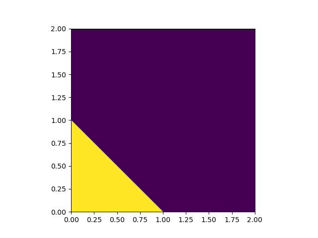

Indeed, we see that the set in this case is not attractive and the evolution of the dominating trait takes a turn from going horizontally to going vertically in trait space upon encountering the line (Figure 6 (right)). We chose such that we do not have a point exactly on the set since this might cause problems with the fitness of both mutant traits being identical (as the derivatives of the fitness are equal).
Example 3.7.
Now, let , , and we consider the competition kernel . Now computing the curve at which the coordinates of agree, we find that this is the case for . Also, we see from Figure 7 (left), that this curve is attractive for . Again, there is no evolutionary singular strategy and hence the population will evolve to the most beneficial trait, this time being . The path taken from the initial trait in the bottom left corner of the trait space to the final trait in the upper right corner is quite different from the one in the previous example.
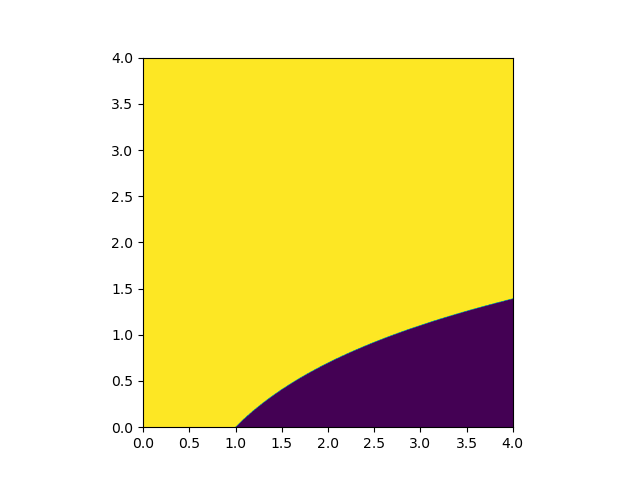

We plot the Euclidean difference of the solution to the canonical equation from Theorem 3.2 and the resident trait from our simulation in Figure 8. To improve legibility of this figure, we calculate the difference only at the times when the function has jumps and interpolate these errors.
As expected, the error is limited by which is the furthest distance we should see on a grid from a smooth curve. Interestingly however, we see that at first we have a negligible error until we encounter the critical curve . Here, the error is erratic since jumps crossing the curve may increase the distance from the curve. As soon as we reach the boundary of our trait space though, the error is smooth again but remains at a non-negligible level due to the -grid not being exactly on the edge of the trait space. When both processes reach the upper right corner of the trait space, the error remains at a constant level.
Appendix A Technical details for the simulations
Here, we give a short summary of the techniques used to create our examples.
A.1. Simulations in one dimension
The solution of the canonical equation in Figure 3 was computed by using a simple Euler method and computing the partial derivative of the fitness function by setting for . For the function , we used the explicit form detailed before Theorem 2.6.
For Figure 4 we require the computation of the coexistence equilibria. In accordance with Assumption 2, we used a damped Newton method with damping factor and initial condition composed of the old equilibrium population for previously resident traits and a small starting population of for invading mutant traits. Computations for the equilibrium were done for at most iterations.
A.2. Simulations in two dimensions
The inequality plots for Figures 6 and 7 were computed on a grid on the square and respectively by calculating the approximate gradient again using with for each of the grid points. If the difference of the components was less than , they were set to be equal.
The plots showing the path of the resident trait in trait space again required the calculation of various equilibria. Thse were done as for the evolutionary branching images.
To calculate the error in Figure 8, we first explicitly computed the speed at which we move along the curve . This is given in Theorem 3.2 as
For it is easy to compute . The tangent at the point is the line uniquely determined by
In particular, the angle with the positive real line is . Plugging this into the formula for the speed at which we move along and normalizing the tangent vector, we obtain
Then we separated the three phases and solved that canonical equation piecewise using an Euler scheme with on a time horizon of . Having simulated the times at which the resident trait changes, we compared the discrepancy of the simulated resident trait at these times (accelerated by ) and the solution of the canonical equation.
Acknowledgements
The author wants to thank M. Wilke Berenguer for helpful comments on an earlier version of this paper. This work was funded by the Deutsche Forschungsgemeinschaft (DFG, German Research Foundation) under Germany’s Excellence Strategy MATH+: The Berlin Mathematics Research Center, EXC-2046/1 project-ID 390685689.
References
- [BB18] M. Baar and A. Bovier, The polymorphic evolution sequence for populations with phenotypic plasticity Electron. J. Probab. 23, 1–27 (2018).
- [BBC17] M. Baar, A. Bovier and N. Champagnat, From stochastic, individual-based models to the canonical equation of adaptive dynamics in one step Ann. Appl. Probab. 27(2), 1093–1170 (2017).
- [BCS19] A.Bovier, L. Coquille and C. Smadi, Crossing a fitness valley as a metastable transition in a stochastic population model Ann. Appl. Probab. 29(6), 3541-3589 (2019).
- [BCM+16] M. Baar, L. Coquille, H. Meyer et al., A stochastic model for immunotherapy of cancer Sci. Rep. 6(24169), (2016).
- [BPT23] J.Blath, T. Paul and A. Tóbiás, A stochastic adaptive dynamics model for bacterial populations with mutation, dormancy and transfer ALEA Lat. Am. J. of Prob. Math. Stat., 20, 313-357 (2023)
- [C06] N. Champagnat, A microscopic interpretation for adaptive dynamics trait substitution sequence models Stoch. Proc. Appl. 116(8), 1127–1160 (2006).
- [CFB01] N. Champagnat, R. Ferrière and G. Ben Arous The canonical equation of adaptive dynamics: a mathematical view Selection 2, 73–83 (2001).
- [CH23] N. Champagnat and V. Hass, Convergence of individual-based models with small and frequent mutations to the canonical equation of adaptive dynamics Arxiv preprint arXiv:2303.09936, (2023).
- [CKS21] L. Coquille, A. Kraut and C. Smadi, Stochastic individual-based models with power law mutation rate on a general finite trait space Electron. J. Prob. 26, 1-37 (2021).
- [CM11] N. Champagnat and S. Méléard, Polymorphic evolution sequence and evolutionary branching Probab. Theory Relat. Fields 151, 45–94 (2011).
- [CMT21] N. Champagnat, S. Méléard and V. C. Tran, Stochastic analysis of emergence of evolutionary cyclic behavior in population dynamics with transfer Ann. Appl. Prob. 31(4), 1820–1867 (2021).
- [CMT23] N. Champagnat, S. Méléard and V. C. Tran, Multi-scale eco-evolutionary models: from individuals to populations ICM 2022 Proceedings to appear (2023).
- [DD99] U. Dieckmann and M. Doebeli, On the origin of species by sympatric speciation Nature 400, 354-357 (1999).
- [DL96] U. Dieckmann and R. Law, The dynamical theory of coevolution: a derivation from stochastic ecological processes J. Math. Biol. 34, 579–612 (1996).
- [DM11] R. Durrett and J. Mayberry, Traveling waves of selective sweeps Ann. Appl. Prob. 21(2), 699–744 (2011).
- [MGM+96] J. A. J. Metz, S. A. H. Geritz, G. Meszéna et al., Adaptive dynamics, a geometrical study of the consequences of nearly faithful reproduction Stochastic and Spatial Structures of Dynamical Systems 45, 183-231 (1996).
- [S17] C. Smadi, The Effect of Recurrent Mutations on Genetic Diversity in a Large Population of Varying Size Acta Appl. Math. 149, 11-51 (2017).