跳到论文正文
W Papers独立论文阅读器 arXiv:2309.02131 论文正文 计算阅读时间 · 0%
引用这篇论文根据当前论文元数据生成,正式投稿前建议核对。


Complex Box SplinesThanks: 1Corresponding author

Fabio Marcelo Carvalho dos Santos Address: Department of Mathematics, Technical University of Munich, Boltzmannstr. 3, 85748 Garching b. Munich, Germany Email address: ge37dey@mytum.de and Peter Massopust1 Address: Department of Mathematics, Technical University of Munich, Boltzmannstr. 3, 85748 Garching b. Munich, Germany Email address: massopust@ma.tum.de
Abstract.

The novel concept of box spline of complex degree is introduced and several of its properties derived and discussed. These box splines of complex degree generalize and extend the classical box splines. Relations to a class of fractional derivatives defined on certain function spaces are also exhibited.

Keywords and Phrases: Complex B-splines, complex truncated power functions, box splines, fractional differential operators, distributions

AMS Subject Classification (2020): 41A15, 26A33, 46F10, 65D07

1. Introduction

The mathematical concept of splines has been a fertile ground for research and innovation, with complex B-splines and box splines being two prominent areas of study. Both have found applications in various domains, such as computer graphics, image and signal processing, and numerical analysis. However, the intersection of these two concepts, known as box splines of complex degree, for short, complex box splines presents an unexplored opportunity with potentially far-reaching implications.

The motivation behind this paper lies in the fusion of these two powerful mathematical constructs. By introducing complex box splines, this research aims to harness the strengths of both complex B-splines and box splines, creating a novel mathematical tool that could transform the way multivariate analysis is approached. While the potential applications of this concept are vast, the focus of this paper is strictly on the theoretical aspects and foundations of complex box splines. This includes the mathematical properties, construction techniques, and underlying theoretical principles. The aim is to create a comprehensive theoretical framework that bridges the gap between complex B-splines and box splines. Moreover, the existing literature, while rich in individual explorations of complex B-splines and box splines, lacks a unified theoretical study that connects these two areas. This paper seeks to fill this void, providing a systematic and purely theoretical approach to understanding complex box splines.

The first inspiration comes from the paper [14] which introduces fractional box splines, the real counterparts to complex box splines, and an extension of the traditional concept. The aforementioned work explores the mathematical intricacies of fractional box splines, opening new perspectives. Amongst others, this approach will be extended to complex degrees.

The second key inspiration is drawn from the paper [2] in which complex B-splines, more precisely cardinal polynomial B-splines of complex degree, were first introduced as a means of adding phase information to the approximants, thus creating a complex-valued transform for the purposes of signal and image analysis. (See [5], for a discussion of the effectiveness of such complex-valued transforms.) In [7], it was shown that complex B-splines are solutions of certain distributional fractional differential equations. A similar representation is derived in this paper for complex box splines extending the mathematical framework and forging a new path in the exploration of these mathematical constructs.

The novel complex box splines allow the approximation of functions in ℝd\mathbb{R}^{d}, d∈ℕd\in\mathbb{N}, which have varying degrees of smoothness along different directions. Here, the reference [14] comes to bear. However, at each point in ℝd\mathbb{R}^{d}, the complex box spline also assigns a direction on the unit sphere of ℝd\mathbb{R}^{d} arising from the imaginary parts of the complex degrees. Data that require such directions can, for instance, be found in geophysics and are known as S (shear), L (Love) and R (Rayleigh) waves. Hence, complex box splines provide a higher-dimensional complex-valued transform.

The structure of this paper is as follows. In Section 2, complex truncated power functions and complex B-splines are reviewed and the properties discussed that are relevant for the purposes of this paper. The next section gives a brief summary of box splines and F-box splines using a distributional approach. Section 4 then defines multivariate truncated complex powers and complex box splines. Here, several relations between these two concepts are derived and their properties described. In Section 5, the relationship between complex box splines and a certain type of fractional derivative is exhibited demonstrating the flexibility of this new class of multivariate approximants.

2. Complex Truncated Power Functions and Complex B-Splines

In this section, we briefly review some of the properties of complex backward difference operators and complex B-splines. We also introduce complex one-dimensional truncated power functions whose extension to higher dimensions plays an important role later when complex box splines are defined.

Throughout this paper, the set of natural numbers is denoted by ℕ:={0,1,2,…}\mathbb{N}:=\{0,1,2,\ldots\}. We also set ℕn:={0,1,…,n}\mathbb{N}_{n}:=\{0,1,\ldots,n\}.

2.1. Complex Backward Difference Operator

In contrast to the approach taken when defining traditional B-splines, we introduce the complex backward difference operator directly in the setting of tempered distributions, rather than first defining it in the time domain. The reason for this choice is that it provides a more direct and streamlined exposition in the context of complex B-splines. This approach also allows us to immediately utilize the powerful and flexible framework provided by the theory of tempered distributions. Furthermore, this approach aligns well with the goal of this paper, which emphasizes the use of distribution theory in studying box splines. The references for this section are [2, 6, 7].

Definition 2.1 (Complex Backward Difference Operator).

Let TT be a tempered distribution on ℝ\mathbb{R} and zz be a complex number with Re(z)>−1\mathop{\mathrm{Re}}(z)>-1. The complex backward difference operator ∇z+1\nabla^{z+1} of degree z+1z+1 is defined as

⟨∇z+1T,φ⟩≔∑k≥0(−1)k​(z+1k)​⟨τk​T,φ⟩=∑k≥0(−1)k​(z+1k)​⟨T,τ−k​φ⟩,\left\langle\nabla^{z+1}T,\varphi\right\rangle\coloneqq\sum_{k\geq 0}(-1)^{k}\binom{z+1}{k}\left\langle\tau_{k}T,\varphi\right\rangle=\sum_{k\geq 0}(-1)^{k}\binom{z+1}{k}\left\langle T,\tau_{-k}\varphi\right\rangle,

where τ−kφ:=φ(⋅+k)\tau_{-k}\varphi:=\varphi(\cdot+k) and φ∈𝒮⁡(ℝ)\varphi\in\mathcal{S}(\mathbb{R}).

Proposition 2.1.

The complex backward difference operator is well-defined for tempered distributions.

Proof.

We need to ensure that the series defining the complex backward difference operator is absolutely convergent in order to apply linearity. Notice that

∑k≥0|(z+1k)|<∞.\sum_{k\geq 0}\left|{\binom{z+1}{k}}\right|<\infty.

Indeed, for large |z|\left|{z}\right|, we have the following asymptotic behavior of the Gamma function:

Γ⁡(z+a)Γ⁡(z+b)=za−b+O⁡(|z|−1),\frac{\Gamma(z+a)}{\Gamma(z+b)}=z^{a-b}+O(\left|{z}\right|^{-1}),

for any curve that joins z=0z=0 and z=∞z=\infty. Thus,

(z+1k)=Γ⁡(z+2)Γ⁡(k+1)​Γ​(z+2−k)=1Γ⁡(k+1)​zk​(1+O⁡(|z|−1)CLOSE,\binom{z+1}{k}=\frac{\Gamma(z+2)}{\Gamma(k+1)\Gamma(z+2-k)}=\frac{1}{\Gamma(k+1)}z^{k}(1+O(\left|{z}\right|^{-1}),

wich implies

∑k≥0|(z+1k)|∑k≥0|1Γ⁡(k+1)zk(1+O(|z|−1)|≤Ce|z|−1,\sum_{k\geq 0}\left|{\binom{z+1}{k}}\right|\sum_{k\geq 0}\left|{\frac{1}{\Gamma(k+1)}z^{k}(1+O(\left|{z}\right|^{-1})}\right|\leq Ce^{\left|{z}\right|^{-1}},

where the last inequality follows from the Taylor expansion of the exponential function and C>0C>0 is some constant. ∎

The next proposition derives an expression for the Fourier transform of the complex difference operator which provides insights into its behavior. (See also, [13] for a derivation for real zz and [2] where the extension to complex zz is stated.) We use the following form of the Fourier transform of f∈L1​(ℝ)f\in L^{1}(\mathbb{R}),

f^​(ω):=∫ℝnf⁡(x)​e−i​ω​x​𝑑x,\widehat{f}(\omega):=\int_{\mathbb{R}^{n}}f(x)e^{-i\omega x}\,dx,

and extend it in the usual way to tempered distributions.

Proposition 2.2 (Fourier Transform of Complex Difference Operators).

Let TT be a tempered distribution on ℝ\mathbb{R}. Then

(2.1) ⟨∇z+1T^,φ⁡(ω)⟩=∑k≥0(−1)k​(z+1k)​⟨e−i​k​ω​T^,φ⁡(ω)⟩,\left\langle{\widehat{\nabla^{z+1}T}},\varphi(\omega)\right\rangle=\sum_{k\geq 0}(-1)^{k}\binom{z+1}{k}\left\langle e^{-ik\omega}{\widehat{T}},\varphi(\omega)\right\rangle,

where φ∈𝒮⁡(ℝ)\varphi\in\mathcal{S}(\mathbb{R}).

Note: On occasion and in abuse of notation, we write the argument of a test function into the pairing if it clarifies the meaning of an expression.

Proof.

As ∑k≥0|(z+1k)|<∞\sum\limits_{k\geq 0}\left|{\binom{z+1}{k}}\right|<\infty and the Fourier transform is linear, we have that

⟨∇z+1T^,φ⁡(ω)⟩\displaystyle\left\langle{\widehat{\nabla^{z+1}T}},\varphi(\omega)\right\rangle =∑k≥0(−1)k​(z+1k)​⟨τk​T^,φ⁡(ω)⟩\displaystyle=\sum_{k\geq 0}(-1)^{k}\binom{z+1}{k}\left\langle\tau_{k}{\widehat{T}},\varphi(\omega)\right\rangle
=∑k≥0(−1)k​(z+1k)​⟨e−i​k​ω​T^,φ⁡(ω)⟩.\displaystyle=\sum_{k\geq 0}(-1)^{k}\binom{z+1}{k}\left\langle e^{-ik\omega}{\widehat{T}},\varphi(\omega)\right\rangle.

∎

We summarize some properties of complex difference operators and refer to [2] for their proofs.

Proposition 2.3 (Properties of Complex Difference Operators).

The complex backward difference operator satisfies the following properties:

  1. (i)

    If TT is a tempered distribution on ℝ\mathbb{R}, then

    (2.2) ⟨∇z+1(t​T),φ⟩=⟨(z+1)​∇zT,φ⟩+⟨[t−(z+1)]​∇z+1T,φ⟩.\left\langle\nabla^{z+1}(tT),\varphi\right\rangle=\left\langle(z+1)\nabla^{z}T,\varphi\right\rangle+\left\langle[t-(z+1)]\nabla^{z+1}T,\varphi\right\rangle.
  2. (ii)

    If T1T_{1} and T2T_{2} are tempered distributions on ℝ\mathbb{R}, then

    (2.3) ⟨∇(z1+1)+(z2+1)(T1∗T2),φ⟩=⟨∇z1+1T1∗∇z2+1T2,φ⟩.\left\langle\nabla^{(z_{1}+1)+(z_{2}+1)}(T_{1}\ast T_{2}),\varphi\right\rangle=\left\langle\nabla^{z_{1}+1}T_{1}\ast\nabla^{z_{2}+1}T_{2},\varphi\right\rangle.

2.2. Truncated Complex Power Functions

In this section, we will define truncated complex power functions and present those properties which relate to complex B-splines and later to complex box splines.

We extend the truncated power function t↦t+nt\mapsto t_{+}^{n} to a complex degree zz by setting

t+z≔{tz=ez​log⁡(t)=tRe(z)​ei​Im(z)​log⁡(t),if t>0;0,else.t_{+}^{z}\coloneqq\begin{cases}t^{z}=e^{z\log(t)}=t^{\mathop{\mathrm{Re}}(z)}e^{i\mathop{\mathrm{Im}}(z)\log(t)},&\text{if $t>0$};\\ 0,&\text{else}.\end{cases}
Refer to caption
Figure 1. Truncated complex power function with z=1+i​γz=1+i\gamma for γ∈[0,2]\gamma\in[0,2].

The next result is a straightforward consequence of the definition of the complex truncated power function. The easy proof is left to the reader.

Theorem 2.1.

For Re(z)≥0\mathop{\mathrm{Re}}(z)\geq 0, we have

t+z∈C⌊Re(z)⌋​(ℝ),t_{+}^{z}\in C^{\left\lfloor\mathop{\mathrm{Re}}(z)\right\rfloor}(\mathbb{R}),

where ⌊⋅⌋\left\lfloor\cdot\right\rfloor denotes the floor function.

t+zt_{+}^{z} induces a tempered distribution on ℝ\mathbb{R} by setting

(2.4) ⟨t+z,φ⁡(t)⟩:=∫0∞tz​φ​(t)​𝑑t,\left\langle t_{+}^{z},\varphi(t)\right\rangle:=\int_{0}^{\infty}t^{z}\varphi(t)dt,

where φ∈𝒮⁡(ℝ)\varphi\in\mathcal{S}(\mathbb{R}). As t+zt_{+}^{z} is locally integrable for Re(z)>−1\mathop{\mathrm{Re}}(z)>-1, the integral is well-defined for Re(z)>−1\mathop{\mathrm{Re}}(z)>-1.

Proposition 2.4 (Weak Derivative of Truncated Complex Powers [8]).

For −1<Re(z)<0-1<\mathop{\mathrm{Re}}(z)<0, we have

(2.5) ⟨D​t+z,φ⁡(t)⟩=⟨z​t+z−1,φ⁡(t)−φ⁡(0)⟩\left\langle Dt_{+}^{z},\varphi(t)\right\rangle=\left\langle zt_{+}^{z-1},\varphi(t)-\varphi(0)\right\rangle

where DD denotes the ordinary derivative.

Remark 2.1.
  1. (i)

    If we consider φ∈𝒮⁡(ℝ)\varphi\in\mathcal{S}(\mathbb{R}) with the additional condition φ⁡(0)=0\varphi(0)=0, a significant simplification occurs:

    (2.6) ⟨D​t+z,φ⁡(t)⟩=⟨z​t+z−1,φ⁡(t)⟩.\left\langle Dt_{+}^{z},\varphi(t)\right\rangle=\left\langle zt_{+}^{z-1},\varphi(t)\right\rangle.

    This yields the usual result for the derivative of t+zt_{+}^{z} in the distributional sense. This choice of test functions that vanish at zero may seem restrictive, but it will serve as an essential cornerstone for the forthcoming developments in later sections.

  2. (ii)

    In the broader context of distributions, the truncated power function t+zt_{+}^{z} can be analytically continued to hold for any complex power, except at non-positive integers where it exhibits poles. This is achieved by employing a method of regularization which allows us to extend the definition of the function into regions where the original integral representation may not converge.

    The thusly normalized function t+zΓ⁡(z+1)\frac{t_{+}^{z}}{\Gamma(z+1)} will be denoted by kz​(t)k_{z}(t). From this point on, we refer to kzk_{z} as the truncated complex power function. Note that

    D​kz​(t)=z​t+z−1Γ⁡(z+1)=kz−1​(t)Dk_{z}(t)=\frac{zt_{+}^{z-1}}{\Gamma(z+1)}=k_{z-1}(t)
Refer to caption
Figure 2. Normalized truncated complex power function with z=1+i​γz=1+i\gamma for γ∈[0,2]\gamma\in[0,2].

Given that complex B-splines will be constructed using truncated complex power functions, much like the cardinal B-splines in the integer case, knowing the Fourier transform of these building blocks is a crucial step in characterizing the spectral properties of the complex B-splines and later the complex box splines themselves.

Proposition 2.5 (Fourier Transform of Truncated Complex Powers [2]).

For Re(z)>−1\mathop{\mathrm{Re}}(z)>-1, Re(z)∉ℕ\mathop{\mathrm{Re}}(z)\notin\mathbb{N}, and Im(z)≠0\mathop{\mathrm{Im}}(z)\neq 0, the Fourier transform of the truncated complex power function is given by

(2.7) ⟨kz^,φ⟩=⟨1(i​ω)z+1,φ⁡(ω)⟩.\left\langle{\widehat{k_{z}}},\varphi\right\rangle=\left\langle\frac{1}{(i\omega)^{z+1}},\varphi(\omega)\right\rangle.

The next result whose proof can be found in [10] plays an important role in the later investigations.

Proposition 2.6 (Convolution of Truncated Complex Power Functions).

Let z1,z2∈ℂz_{1},z_{2}\in\mathbb{C} with Re(zj)>−1\mathop{\mathrm{Re}}(z_{j})>-1 for j=1,2j=1,2. Then

(2.8) ⟨kz1∗kz2,φ⟩=⟨kz1+z2+1,φ⟩,\left\langle k_{z_{1}}\ast k_{z_{2}},\varphi\right\rangle=\left\langle k_{z_{1}+z_{2}+1},\varphi\right\rangle,

with φ∈𝒮⁡(ℝ)\varphi\in\mathcal{S}(\mathbb{R}).

2.3. Review of Complex B-Splines

Complex B-splines were first introduced in [2] and later investigated in a albeit incomplete series of papers [1, 6, 7, 9]. The original definition was based on the Fourier transform but for our purposes we present in this section an alternate but equivalent definition via complex truncated power functions. Moreover, our definition employs a distributional setting.

Definition 2.2 (Complex B-Splines).

Let Re(z)>−1\mathop{\mathrm{Re}}(z)>-1. The complex B-spline BzB_{z} of degree zz is defined as the tempered distribution given by

(2.9) ⟨Bz,φ⟩:=⟨∇z+1kz,φ⟩,\left\langle B_{z},\varphi\right\rangle:=\left\langle\nabla^{z+1}k_{z},\varphi\right\rangle,

with φ∈𝒮⁡(ℝ)\varphi\in\mathcal{S}(\mathbb{R}).

In the next proposition, we list some properties of complex B-splines in the distributional setting. Proofs in the non-distributional setting can be found in [2]; the extension to the distributional setting is based on the distributional definitions of the complex backward difference operator and complex truncated power function. The details are left to the reader.

Proposition 2.7 (Properties of Complex B-Splines).

Complex B-splines enjoy the following properties:

  1. (i)

    The complex B-spline satisfies the convolution property

    ⟨Bz1∗Bz2,φ⟩=⟨Bz1+z2+1,φ⟩,\left\langle B_{z_{1}}\ast B_{z_{2}},\varphi\right\rangle=\left\langle B_{z_{1}+z_{2}+1},\varphi\right\rangle,

    with Re(zj)>−1\mathop{\mathrm{Re}}(z_{j})>-1 for j=1,2j=1,2.

  2. (ii)

    The complex B-spline satisfies the recurrence relation

    ⟨Bz,φ⟩=⟨tz​Bz−1+z+1−tz​τ1​Bz−1,φ⟩,\left\langle B_{z},\varphi\right\rangle=\left\langle\frac{t}{z}B_{z-1}+\frac{z+1-t}{z}\tau_{1}B_{z-1},\varphi\right\rangle,

    with Re(z)>0\mathop{\mathrm{Re}}(z)>0.

  3. (iii)

    The Fourier transform of the complex B-spline BzB_{z} is given by the tempered distribution

    (2.10) ⟨Bz^​(ω),φ⁡(ω)⟩=⟨(1−e−i​ωi​ω)z+1,φ⁡(ω)⟩,\left\langle{\widehat{B_{z}}}(\omega),\varphi(\omega)\right\rangle=\left\langle\left(\frac{1-e^{-i\omega}}{i\omega}\right)^{z+1},\varphi(\omega)\right\rangle,

    with φ∈𝒮⁡(ℝ)\varphi\in\mathcal{S}(\mathbb{R}).

  4. (iv)

    The Fourier transform Bz^{\widehat{B_{z}}} of a complex B-spline can be identified with an L2​(ℝ)L^{2}(\mathbb{R}) function if Re(z)>−12\mathop{\mathrm{Re}}(z)>-\frac{1}{2}. Thus, by Parseval’s identity, Bz∈L2​(ℝ)B_{z}\in L^{2}(\mathbb{R}) if Re(z)>−12\mathop{\mathrm{Re}}(z)>-\frac{1}{2}

Note, that the spectrum of a complex B-spline Bz^{\widehat{B_{z}}} consists of the spectrum of a so-called fractional B-spline [13], combined with a modulation and a damping factor:

(2.11) Bz^​(ω)=BRe⁡z^​(ω)​ei​Im⁡z​ln⁡Ω​(ω)​e−Im⁡z​arg⁡Ω​(ω).{\widehat{B_{z}}(\omega)}={\widehat{B_{\re z}}(\omega)}\,e^{i\im z\ln\Omega(\omega)}\,e^{-\im z\arg\Omega(\omega)}.

where Ω⁡(ω):=1−e−i​ωi​ω\Omega(\omega):=\frac{1-e^{-i\omega}}{i\omega}.

For further properties of complex B-splines, we refer the interested reader to the albeit incomplete list of papers given at the beginning of this subsection.

3. Box Splines

For the purposes of notation and terminology, we present a brief introduction to box splines in this section. For more details, we refer the interested reader to, for instance, [3, 4] and the references given therein.

Definition 3.1 (Direction Set).

Let n∈ℕn\in\mathbb{N}. A direction set Mn+1M_{n+1} is a d×(n+1)d\times(n+1) matrix with columns (m0,m1,…,mn)(m_{0},m_{1},\ldots,m_{n}), all in ℝd\0\mathbb{R}^{d}\backslash 0, such that

span⁡(Mn+1)=ℝd.\mathrm{span\,}(M_{n+1})=\mathbb{R}^{d}.

Direction sets are used to define box splines.

Definition 3.2 (Box Spline).

Let M=[m0,m1,…,mn]M=[m_{0},m_{1},\ldots,m_{n}] be a matrix whose columns mjm_{j} form a direction set. The box spline BMB_{M} associated with the matrix MM is defined to be the tempered distribution

BM:𝒮⁡(ℝd)\displaystyle B_{M}:\mathcal{S}(\mathbb{R}^{d}) →ℝ\displaystyle\rightarrow\mathbb{R}
φ\displaystyle\varphi ↦⟨BM,φ⟩≔∫[0,1)n+1φ(Mt)dt.\displaystyle\mapsto\left\langle B_{M},\varphi\right\rangle\coloneqq\int_{[0,1)^{n+1}}\varphi(Mt)dt.

The definition of the box spline BMB_{M} can be understood geometrically as a mapping that measures the ’average’ value of φ\varphi over the parallelepiped defined by the direction set. This is a natural extension of the univariate case, where the B-spline measures the average value of a test function over an interval.

In [14], a generalization of box spline was presented by including a function ff that will serve as a weight. These so-called F-box splines Bf(⋅|M)B_{f}(\cdot|M) are tempered distributions defined by

(3.1) Bf(⋅|M):𝒮(ℝd)→ℝφ↦⟨Bf(⋅|M),φ⟩≔∫ℝdBf(x|M)φ(x)dx=∫[0,1)n+1f(t)φ(Mt)dt.\displaystyle\begin{split}B_{f}(\cdot|M):\mathcal{S}(\mathbb{R}^{d})&\rightarrow\mathbb{R}\\ \varphi&\mapsto\left\langle B_{f}(\cdot|M),\varphi\right\rangle\coloneqq\int_{\mathbb{R}^{d}}B_{f}(x|M)\varphi(x)dx=\int_{[0,1)^{n+1}}f(t)\varphi(Mt)dt.\end{split}

This generalization allows us to consider a wider class of functions as weights, thereby enriching the structure and properties of the resulting splines. One particularly interesting and important class of functions that we can consider is the class of complex-valued functions. By choosing a specific weight ff, we can define complex box splines, which is the main focus of this paper.

Multivariate truncated powers [4] are defined within an affine cone with the assumption that the first non-zero component of each vector in the direction set is positive.

Definition 3.3 (Multivariate Truncated Power).

Let MM be an d×(n+1)d\times(n+1) matrix whose columns form a direction set. Multivariate truncated powers TMT_{M} associated with MM are the tempered distributions given by

(3.2) TM:𝒮⁡(ℝd)→ℝφ↦⟨TM,φ⟩≔∫ℝ+n+1φ⁡(M​t)​dt.\displaystyle\begin{split}T_{M}:\mathcal{S}(\mathbb{R}^{d})&\rightarrow\mathbb{R}\\ \varphi&\mapsto\left\langle T_{M},\varphi\right\rangle\coloneqq\int_{\mathbb{R}_{+}^{n+1}}\varphi(Mt)dt.\end{split}

By a weight ff, we obtain multivariate F-truncated powers Tf(⋅|M)T_{f}(\cdot|M):

(3.3) Tf(⋅|M):𝒮(ℝd)→ℝφ↦⟨Tf(⋅|M),φ⟩≔∫ℝdTf(x|M)φ(x)dx=∫ℝ+n+1f(t)φ(Mt)dt.\displaystyle\begin{split}T_{f}(\cdot|M):\mathcal{S}(\mathbb{R}^{d})&\rightarrow\mathbb{R}\\ \varphi&\mapsto\left\langle T_{f}(\cdot|M),\varphi\right\rangle\coloneqq\int_{\mathbb{R}^{d}}T_{f}(x|M)\varphi(x)dx=\int_{\mathbb{R}_{+}^{n+1}}f(t)\varphi(Mt)dt.\end{split}

The multivariate truncated power is closely related to the box spline, as the following theorem suggests.

Theorem 3.1 (Box Spline Representation [4]).

The box spline BMB_{M} can also be defined as

(3.4) ⟨BM,φ⟩=⟨∏j=0n∇mjTM,φ⟩,\left\langle B_{M},\varphi\right\rangle=\left\langle\prod_{j=0}^{n}\nabla_{m_{j}}T_{M},\varphi\right\rangle,

where ∇mj\nabla_{m_{j}} denotes the multivariate backward difference operator with respect to the vector mjm_{j} and is defined as

⟨∇mjTM,φ⟩=⟨TM−τmj​TM,φ⟩,\left\langle\nabla_{m_{j}}T_{M},\varphi\right\rangle=\left\langle T_{M}-\tau_{m_{j}}T_{M},\varphi\right\rangle,

where φ∈𝒮⁡(ℝd)\varphi\in\mathcal{S}(\mathbb{R}^{d}).

Finally, we list some properties of box splines. Proofs can be found in [4].

Proposition 3.1 (Properties of Box Splines).

Box splines have the following properties:

  1. (i)

    supp(BM)=M([0,1)n+1)\mathrm{supp\,}(B_{M})=M([0,1)^{n+1});

  2. (ii)

    Recurrence relation:

    ⟨BM,φ⟩=⟨∫01BM∖mn(⋅−tmn)dt,φ⟩;\left\langle B_{M},\varphi\right\rangle=\left\langle\int_{0}^{1}B_{M\setminus m_{n}}(\cdot-tm_{n})dt,\varphi\right\rangle;
  3. (iii)

    If MM is invertible (i.e. the direction set is a basis of ℝd\mathbb{R}^{d}), then BMB_{M} can be associated with the normalized characteristic function of the parallelepiped M([0,1)n+1)M([0,1)^{n+1}), that it

    BM(t)=1|det(M)|χM([0,1)n+1)(t);B_{M}(t)=\frac{1}{|\det(M)|}\chi_{M([0,1)^{n+1})}(t);
  4. (iv)

    Fourier transform:

    ⟨BM^,φ⟩=⟨∏j=0n1−exp(−iω⋅xj)i​ω⋅xj,φ⟩,\left\langle{\widehat{B_{M}}},\varphi\right\rangle=\left\langle\prod_{j=0}^{n}\frac{1-\exp(-i\omega\cdot x_{j})}{i\omega\cdot x_{j}},\varphi\right\rangle,

    with φ∈𝒮⁡(ℝd)\varphi\in\mathcal{S}(\mathbb{R}^{d}).

  5. (v)

    The convolution of two box splines yields again a box spline:

    ⟨BM∗BN,φ⟩=⟨BM∪N,φ⟩,\left\langle B_{M}\ast B_{N},\varphi\right\rangle=\left\langle B_{M\cup N},\varphi\right\rangle,

    where M∪NM\cup N is the matrix made up of the columns of MM and NN.

4. Complex Box Splines

Complex box splines are a new tool in spline theory, merging the complex degrees of B-splines with the multivariate flexibility of traditional box splines. They are a novel extension of traditional box splines and are characterized by their complex degrees, thus offering a unique perspective on the interplay between geometry and analysis, particularly in the context of multivariate functions and introducing a new multidimensional complex transform.

4.1. Multivariate Truncated Complex Powers

We begin by introducing multivariate truncated complex power functions.

Definition 4.1 (Multivariate Truncated Complex Power Function).

Let MM be an d×(n+1)d\times(n+1) matrix whose columns form a direction set. Set 𝐳≔(z0,z1,…,zn)∈ℂn+1{\boldsymbol{z}}\coloneqq(z_{0},z_{1},\ldots,z_{n})\in\mathbb{C}^{n+1} where Re(zj)>−1\mathop{\mathrm{Re}}(z_{j})>-1 for all j∈ℕnj\in\mathbb{N}_{n} and let

k𝒛​(t)≔t+𝒛Γ⁡(𝒛+1)=∏j=0n(tj)+zjΓ⁡(zj+1).k_{\boldsymbol{z}}(t)\coloneqq\frac{t_{+}^{\boldsymbol{z}}}{\Gamma({\boldsymbol{z}}+1)}=\prod_{j=0}^{n}\frac{(t_{j})_{+}^{z_{j}}}{\Gamma(z_{j}+1)}.

The tempered distribution 𝒯𝐳(⋅|M)≔Tk𝐳(⋅|M)\mathcal{T}_{{\boldsymbol{z}}}(\cdot|M)\coloneqq T_{k_{\boldsymbol{z}}}(\cdot|M),

𝒯𝒛(⋅|M):𝒮(ℝd)\displaystyle\mathcal{T}_{{\boldsymbol{z}}}(\cdot|M):\mathcal{S}(\mathbb{R}^{d}) →ℝ\displaystyle\rightarrow\mathbb{R}
φ\displaystyle\varphi ↦⟨𝒯𝒛(⋅|M),φ⟩≔∫ℝd𝒯𝒛(x|M)φ(x)dx=∫ℝ+n+1k𝒛(t)φ(Mt)dt,\displaystyle\mapsto\left\langle\mathcal{T}_{{\boldsymbol{z}}}(\cdot|M),\varphi\right\rangle\coloneqq\int_{\mathbb{R}^{d}}\mathcal{T}_{{\boldsymbol{z}}}(x|M)\varphi(x)dx=\int_{\mathbb{R}_{+}^{n+1}}k_{\boldsymbol{z}}(t)\varphi(Mt)dt,

is called a multivariate truncated complex power (function).

The next result examines the rate of change of a multivariate complex truncated power distribution in the specific direction defined by an element in the direction set.

Theorem 4.1 (Weak Derivative of Multivariate Truncated Complex Powers).

If Re(zj)>0\mathop{\mathrm{Re}}(z_{j})>0 for all j∈ℕnj\in\mathbb{N}_{n}, then

⟨Dmj𝒯𝒛(⋅|M),φ⟩=⟨𝒯𝒛−ej(⋅|M),φ⟩,\left\langle D_{m_{j}}\mathcal{T}_{{\boldsymbol{z}}}(\cdot|M),\varphi\right\rangle=\left\langle\mathcal{T}_{{\boldsymbol{z}}-e_{j}}(\cdot|M),\varphi\right\rangle,

where eje_{j} denotes one of the canonical basis vector in ℝn+1\mathbb{R}^{n+1}.

Proof.

Let φ∈𝒮⁡(ℝd)\varphi\in\mathcal{S}(\mathbb{R}^{d}). Then,

⟨Dmj​𝒯𝒛​(x|M),φ⁡(x)⟩\displaystyle\left\langle D_{m_{j}}\mathcal{T}_{{\boldsymbol{z}}}(x|M),\varphi(x)\right\rangle =−∫ℝsTk𝒛(x|M)Dmjφ(x)dx\displaystyle=-\int_{\mathbb{R}^{s}}T_{k_{\boldsymbol{z}}}(x|M)D_{m_{j}}\varphi(x)dx
=−∫ℝ+n+1k𝒛(t)∂φ⁡(M​t)∂ujdu\displaystyle=-\int_{\mathbb{R}_{+}^{n+1}}k_{\boldsymbol{z}}(t)\frac{\partial\varphi(Mt)}{\partial u_{j}}du
=∫ℝ+n+1∂∂tj​k𝒛​(t)​φ​(M​t)​𝑑u\displaystyle=\int_{\mathbb{R}_{+}^{n+1}}\frac{\partial}{\partial t_{j}}k_{\boldsymbol{z}}(t)\varphi(Mt)du
=∫ℝ+n+1k𝒛−ej​(t)​φ​(M​t)​𝑑t\displaystyle=\int_{\mathbb{R}_{+}^{n+1}}k_{{\boldsymbol{z}}-e_{j}}(t)\varphi(Mt)dt
=∫ℝdTk𝒛−ej​(x|M)​φ​(x)​𝑑x\displaystyle=\int_{\mathbb{R}^{d}}T_{k_{{\boldsymbol{z}}-e_{j}}}(x|M)\varphi(x)dx
=⟨𝒯𝒛−ej​(x|M),φ⁡(x)⟩,\displaystyle=\left\langle\mathcal{T}_{{\boldsymbol{z}}-e_{j}}(x|M),\varphi(x)\right\rangle,

where we used

∂∂tj​k𝒛​(t)\displaystyle\frac{\partial}{\partial t_{j}}k_{\boldsymbol{z}}(t) =(∂∂tj​kzj​(tj))​∏i≠jn(ti)+ziΓ⁡(zi+1)=(kzj−1​(tj))​∏i≠jn(ti)+ziΓ⁡(zi+1)=k𝒛−ej​(t).∎\displaystyle=\left(\frac{\partial}{\partial t_{j}}k_{z_{j}}(t_{j})\right)\prod_{i\neq j}^{n}\frac{(t_{i})_{+}^{z_{i}}}{\Gamma(z_{i}+1)}=\left(k_{z_{j}-1}(t_{j})\right)\prod_{i\neq j}^{n}\frac{(t_{i})_{+}^{z_{i}}}{\Gamma(z_{i}+1)}=k_{{\boldsymbol{z}}-e_{j}}(t).\qed
Theorem 4.2 (Mixed Weak Derivative of Multivariate Truncated Complex Powers).

If Re(zj)>0\mathop{\mathrm{Re}}(z_{j})>0 for all j∈ℕnj\in\mathbb{N}_{n}, then

⟨DM𝒯𝒛(⋅|M),φ⟩=⟨𝒯𝒛−1(⋅|M),φ⟩,\left\langle D_{M}\mathcal{T}_{{\boldsymbol{z}}}(\cdot|M),\varphi\right\rangle=\left\langle\mathcal{T}_{{\boldsymbol{z}}-1}(\cdot|M),\varphi\right\rangle,

where φ∈𝒮⁡(ℝd)\varphi\in\mathcal{S}(\mathbb{R}^{d}). In this context, DMD_{M} denotes differentiation with respect to all directions specified by the columns of the matrix MM simultaneously, and 𝐳−1{\boldsymbol{z}}-1 denotes the vector obtained by subtracting 1 from each component of 𝐳{\boldsymbol{z}}.

Proof.

The proof follows the same lines as the previous one by noticing that

∂n+1∂t0​∂t1​…​∂tn​k𝒛​(t)=k𝒛−1​(t),\frac{\partial^{n+1}}{\partial t_{0}\partial t_{1}\ldots\partial t_{n}}k_{\boldsymbol{z}}(t)=k_{{\boldsymbol{z}}-1}(t),

as each factor depends on a different variable. ∎

Remark 4.1.

Note that in general mixed partial derivatives may not commute for distributions. In our case, because the distribution arises from a product of truncated complex power functions, the order of differentiation does not change the result, and we can talk about “the” mixed derivative without ambiguity.

This concept of mixed partial derivative allows us to generalize the observation that we made in Proposition 2.5 to the multivariate complex truncated power distribution.

Proposition 4.1.

If −1<Re(zj)<0-1<\mathop{\mathrm{Re}}(z_{j})<0, for all j∈ℕnj\in\mathbb{N}_{n}, then

⟨DMn𝒯𝒛(⋅|M),φ⟩=⟨𝒯𝒛−1(⋅|M),φ(⋅)−φ(0)⟩,\left\langle D_{M_{n}}\mathcal{T}_{{\boldsymbol{z}}}(\cdot|M),\varphi\right\rangle=\left\langle\mathcal{T}_{{\boldsymbol{z}}-1}(\cdot|M),\varphi(\cdot)-\varphi(0)\right\rangle,

where φ∈𝒮⁡(ℝd)\varphi\in\mathcal{S}(\mathbb{R}^{d}).

Proof.

We first observe that since (tj)+zj(t_{j})_{+}^{z_{j}} is locally integrable for Re(zj)>−1\mathop{\mathrm{Re}}(z_{j})>-1, the product of n+1n+1 univariate such functions is also locally integrable as long as Re(zj)>−1\mathop{\mathrm{Re}}(z_{j})>-1, for all j∈ℕnj\in\mathbb{N}_{n}. Therefore, we can use the technique of the univariate case n+1n+1 times. ∎

Theorem 4.3 (Fourier Transform of Multivariate Truncated Complex Powers).

The Fourier transform of a multivariate truncated power is the tempered distribution given by

(4.1) ⟨𝒯𝒛^​(ω|M),φ⁡(ω)⟩=⟨∏j=0n1(i​ω⋅mj)zj+1,φ⁡(ω)⟩.\left\langle{\widehat{\mathcal{T}_{{\boldsymbol{z}}}}}(\omega|M),\varphi(\omega)\right\rangle=\left\langle\prod_{j=0}^{n}\frac{1}{(i\omega\cdot m_{j})^{z_{j}+1}},\varphi(\omega)\right\rangle.
Proof.

Let φ∈𝒮⁡(ℝd)\varphi\in\mathcal{S}(\mathbb{R}^{d}). Then,

⟨𝒯𝒛^​(ω|M),φ​(ω)⟩\displaystyle\left\langle{\widehat{\mathcal{T}_{{\boldsymbol{z}}}}}(\omega|M),\varphi(\omega)\right\rangle =∫ℝd𝒯𝒛^​(ω|M)​φ​(ω)​𝑑ω\displaystyle=\int_{\mathbb{R}^{d}}{\widehat{\mathcal{T}_{{\boldsymbol{z}}}}}(\omega|M)\varphi(\omega)d\omega
=∫ℝd𝒯𝒛​(ω|M)​φ^​(ω)​𝑑ω\displaystyle=\int_{\mathbb{R}^{d}}\mathcal{T}_{{\boldsymbol{z}}}(\omega|M){\widehat{\varphi}}(\omega)d\omega
=∫ℝn+1k𝒛​(t)​φ^​(M​t)​𝑑t\displaystyle=\int_{\mathbb{R}^{n+1}}k_{{\boldsymbol{z}}}(t){\widehat{\varphi}}(Mt)dt
=∫ℝn+1k𝒛(t)(∫ℝdφ(ω)e−i(Mt)⋅ωdω)dt\displaystyle=\int_{\mathbb{R}^{n+1}}k_{{\boldsymbol{z}}}(t)\left(\int_{\mathbb{R}^{d}}\varphi(\omega)e^{-i(Mt)\cdot\omega}d\omega\right)dt
=∫ℝd(∫ℝ+n+1k𝒛(t)e−i(Mt)⋅ωdt)φ(ω)dω\displaystyle=\int_{\mathbb{R}^{d}}\left(\int_{\mathbb{R}_{+}^{n+1}}k_{{\boldsymbol{z}}}(t)e^{-i(Mt)\cdot\omega}dt\right)\varphi(\omega)d\omega
=∫ℝd(∫ℝ+n+1∏j=0nkzj(tj)exp(−i∑j=0n(ω⋅mj)tj)dtj)φ(ω)dω\displaystyle=\int_{\mathbb{R}^{d}}\left(\int_{\mathbb{R}_{+}^{n+1}}\prod_{j=0}^{n}k_{z_{j}}(t_{j})\exp\left(-i\sum_{j=0}^{n}(\omega\cdot m_{j})t_{j}\right)dt_{j}\right)\varphi(\omega)d\omega
=∫ℝd(∏j=0n∫ℝ+kzj​(tj)​e−i​tj​(ω⋅mj)​d​tj)​φ​(ω)​𝑑ω,\displaystyle=\int_{\mathbb{R}^{d}}\left(\prod_{j=0}^{n}\int_{\mathbb{R}_{+}}k_{z_{j}}(t_{j})e^{-it_{j}(\omega\cdot m_{j})}dt_{j}\right)\varphi(\omega)d\omega,

where we have used the Fubini-Tonelli theorem. Using the Fourier transform of the truncated complex power yields

⟨𝒯𝒛^​(ω|M),φ⁡(ω)⟩=⟨∏j=0n1(i​ω⋅mj)zj+1,φ⁡(ω)⟩,φ∈𝒮⁡(ℝd).∎\left\langle{\widehat{\mathcal{T}_{{\boldsymbol{z}}}}}(\omega|M),\varphi(\omega)\right\rangle=\left\langle\prod_{j=0}^{n}\frac{1}{(i\omega\cdot m_{j})^{z_{j}+1}},\varphi(\omega)\right\rangle,\quad\varphi\in\mathcal{S}(\mathbb{R}^{d}).\qed

We now can turn our attention to the convolution of multivariate truncated complex powers, which is a natural extension of Proposition 2.6. However, we need to be careful about what convolution means when a direction set comes into play. Indeed, a similar convolution property as in the univariate case will hold, but the resulting multivariate truncated complex power will be defined on the union of both direction sets. In order to simplify notation, we will assume that both multivariate truncated complex powers will be defined over the same direction set or the second over a subset of the first one.

Proposition 4.2 (Convolution of Multivariate Truncated Complex Powers).

Let 𝐳,𝐳¯∈ℂn+1{\boldsymbol{z}},\overline{{\boldsymbol{z}}}\in\mathbb{C}^{n+1} with Re(zj)>−1\mathop{\mathrm{Re}}(z_{j})>-1 and Re(zj¯)>−1\mathop{\mathrm{Re}}(\overline{z_{j}})>-1 for j∈ℕnj\in\mathbb{N}_{n}. Then

(4.2) ⟨𝒯𝒛(⋅|M)∗𝒯𝒛¯(⋅|M),φ⟩=⟨𝒯𝒛+𝒛¯+1(⋅|M),φ⟩,\left\langle\mathcal{T}_{{\boldsymbol{z}}}(\cdot|M)\ast\mathcal{T}_{\overline{{\boldsymbol{z}}}}(\cdot|M),\varphi\right\rangle=\left\langle\mathcal{T}_{{\boldsymbol{z}}+\overline{{\boldsymbol{z}}}+1}(\cdot|M),\varphi\right\rangle,

with φ∈𝒮⁡(ℝd)\varphi\in\mathcal{S}(\mathbb{R}^{d}).

Proof.

Taking the Fourier transform on the left-hand side yields

⟨𝒯𝒛(⋅|M)∗𝒯𝒛¯(⋅|M),φ⟩=⟨𝒯𝒛^(ω|M)⋅𝒯𝒛¯^(ω|M),φ(ω)⟩.\left\langle\mathcal{T}_{{\boldsymbol{z}}}(\cdot|M)\ast\mathcal{T}_{\overline{{\boldsymbol{z}}}}(\cdot|M),\varphi\right\rangle=\left\langle{\widehat{\mathcal{T}_{{\boldsymbol{z}}}}}(\omega|M)\cdot{\widehat{\mathcal{T}_{\overline{{\boldsymbol{z}}}}}}(\omega|M),\varphi(\omega)\right\rangle.

Now, using the expression of the Fourier transform given in (4.1) produces

⟨𝒯𝒛^​(ω|M)⋅𝒯𝒛¯^​(ω|M),φ⁡(ω)⟩=⟨∏j=0n1(i​ω⋅mj)(zj+1)+(zj¯+1),φ⁡(ω)⟩.\left\langle{\widehat{\mathcal{T}_{{\boldsymbol{z}}}}}(\omega|M)\cdot{\widehat{\mathcal{T}_{\overline{{\boldsymbol{z}}}}}}(\omega|M),\varphi(\omega)\right\rangle=\left\langle\prod_{j=0}^{n}\frac{1}{(i\omega\cdot m_{j})^{(z_{j}+1)+(\overline{z_{j}}+1)}},\varphi(\omega)\right\rangle.

Finally, Fourier inversion gives

⟨𝒯𝒛(⋅|M)∗𝒯𝒛¯(⋅|M),φ⟩=⟨𝒯𝒛+𝒛¯+1(⋅|M),φ⟩.∎\left\langle\mathcal{T}_{{\boldsymbol{z}}}(\cdot|M)\ast\mathcal{T}_{\overline{{\boldsymbol{z}}}}(\cdot|M),\varphi\right\rangle=\left\langle\mathcal{T}_{{\boldsymbol{z}}+\overline{{\boldsymbol{z}}}+1}(\cdot|M),\varphi\right\rangle.\qed

4.2. Introducing Complex Box Splines

We now can proceed to the definition of complex box splines. The idea is based on F-box splines 3.1 with a suitable candidate for the weight ff.

Definition 4.2 (Complex Box Splines).

Let MM be an d×(n+1)d\times(n+1) matrix whose columns form a direction set. Let 𝐳≔(z0,z1,…,zn)∈ℂn+1{\boldsymbol{z}}\coloneqq(z_{0},z_{1},\ldots,z_{n})\in\mathbb{C}^{n+1} such that Re(zj)>−1\mathop{\mathrm{Re}}(z_{j})>-1, for all j∈ℕnj\in\mathbb{N}_{n}. Define

B𝒛​(t)≔∏j=0nBzj​(tj),B_{{\boldsymbol{z}}}(t)\coloneqq\prod_{j=0}^{n}B_{z_{j}}(t_{j}),

and

ℬ𝒛(⋅|M)≔TB𝒛(⋅|M).\mathcal{B}_{{\boldsymbol{z}}}(\cdot|M)\coloneqq T_{B_{{\boldsymbol{z}}}}(\cdot|M).

The tempered distribution ℬ𝐳(⋅|M)\mathcal{B}_{{\boldsymbol{z}}}(\cdot|M) given by

(4.3) ℬ𝒛(⋅|M):𝒮(ℝd)\displaystyle\mathcal{B}_{{\boldsymbol{z}}}(\cdot|M):\mathcal{S}(\mathbb{R}^{d}) →ℝ\displaystyle\rightarrow\mathbb{R}
φ\displaystyle\varphi ↦⟨ℬ𝒛(⋅|M),φ⟩≔∫ℝdℬ𝒛(x|M)φ(x)dx=∫ℝ+n+1B𝒛(t)φ(Mt)dt\displaystyle\mapsto\left\langle\mathcal{B}_{{\boldsymbol{z}}}(\cdot|M),\varphi\right\rangle\coloneqq\int_{\mathbb{R}^{d}}\mathcal{B}_{{\boldsymbol{z}}}(x|M)\varphi(x)dx=\int_{\mathbb{R}_{+}^{n+1}}B_{{\boldsymbol{z}}}(t)\varphi(Mt)dt

is called a box spline of complex order 𝐳{\boldsymbol{z}}, for short, a complex box spline.

Note that, unlike in the definition of F-box splines, the integral defining complex box splines is over ℝ+n+1\mathbb{R}_{+}^{n+1}. Indeed, this is due to the fact that complex B-splines are not compactly supported.

Now, assume for a moment that MM is invertible, i.e., the direction set is a basis of ℝd\mathbb{R}^{d}. Set y:=M​ty:=Mt in the definition of complex box spline (4.3). Then, we obtain

⟨ℬ𝒛(y|M),φ(y)⟩=⟨1|det(M)|∫M([0,1)n)B𝒛(M−1y)ϕ(y)dy,φ(y)⟩.\left\langle\mathcal{B}_{\boldsymbol{z}}(y|M),\varphi(y)\right\rangle=\left\langle\frac{1}{\left|{\det(M)}\right|}\int_{M([0,1)^{n})}B_{\boldsymbol{z}}(M^{-1}y)\phi(y)dy,\varphi(y)\right\rangle.

Thus, ℬ𝒛(⋅|M)\mathcal{B}_{\boldsymbol{z}}(\cdot|M) can be identified with the function

(4.4) ℬ𝒛(y|M)=1|det(M)|B𝒛(M−1y)χM([0,1)n)(y),\mathcal{B}_{\boldsymbol{z}}(y|M)=\frac{1}{\left|{\det(M)}\right|}B_{\boldsymbol{z}}(M^{-1}y)\chi_{M([0,1)^{n})}(y),

in the sense that the distribution acts on a test function, as the right-hand side does. Here, χS\chi_{S} denotes the characteristic function of a set SS.

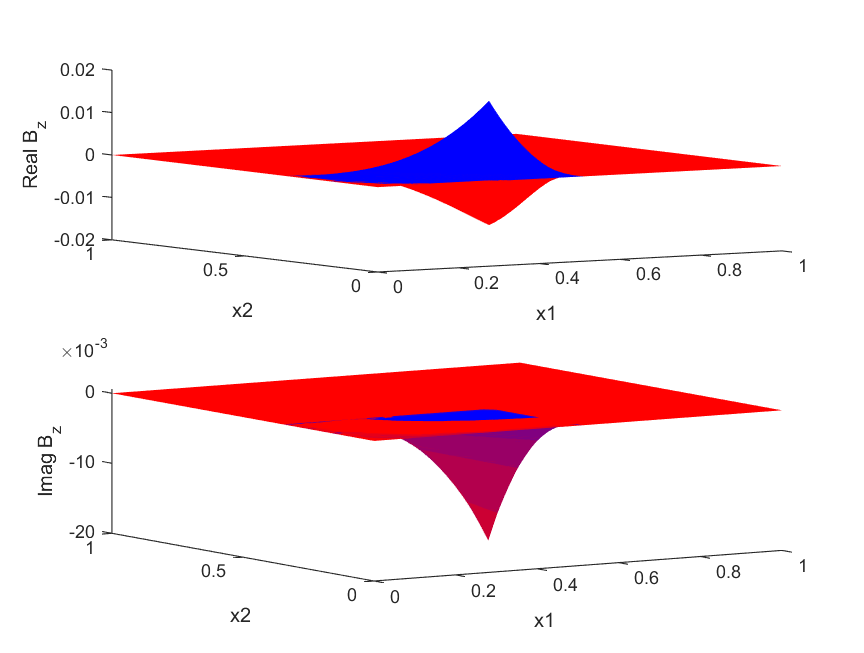
Refer to caption
Figure 3. Real and imaginary parts of the complex box spline with M=(2003)M=\begin{pmatrix}2&0\\ 0&3\end{pmatrix} and z1=3+iz_{1}=3+i, z2=2+iz_{2}=2+i.

The next theorem investigates the weak derivative of complex box splines.

Theorem 4.4 (Weak Derivative of Complex Box Splines).
  1. (i)

    If Re(zj)>0\mathop{\mathrm{Re}}(z_{j})>0, then

    (4.5) ⟨Dmjℬ𝒛(⋅|M),φ⟩=⟨ℬ𝒛−ej(⋅|M)−τmjℬ𝒛−ej(⋅|M),φ⟩.\left\langle D_{m_{j}}\mathcal{B}_{{\boldsymbol{z}}}(\cdot|M),\varphi\right\rangle=\left\langle\mathcal{B}_{{\boldsymbol{z}}-e_{j}}(\cdot|M)-\tau_{m_{j}}\mathcal{B}_{{\boldsymbol{z}}-e_{j}}(\cdot|M),\varphi\right\rangle.
  2. (ii)

    If Re(zj)>k\mathop{\mathrm{Re}}(z_{j})>k, then

    (4.6) ⟨Dmjkℬ𝒛(⋅|M),φ⟩=⟨∑l=0k(−1)l(kl)τj​mjℬ𝒛−k​mj(⋅|M),φ⟩.\left\langle D^{k}_{m_{j}}\mathcal{B}_{{\boldsymbol{z}}}(\cdot|M),\varphi\right\rangle=\left\langle\sum_{l=0}^{k}(-1)^{l}\binom{k}{l}\tau_{jm_{j}}\mathcal{B}_{{\boldsymbol{z}}-km_{j}}(\cdot|M),\varphi\right\rangle.
  3. (iii)

    If Re(zj)>0\mathop{\mathrm{Re}}(z_{j})>0, for all j∈ℕnj\in\mathbb{N}_{n}, then

    (4.7) ⟨DMnℬ𝒛(⋅|M),φ⟩=⟨ℬ𝒛−1(⋅|M)−τ1ℬ𝒛−1(⋅|M),φ⟩.\left\langle D_{M_{n}}\mathcal{B}_{{\boldsymbol{z}}}(\cdot|M),\varphi\right\rangle=\left\langle\mathcal{B}_{{\boldsymbol{z}}-1}(\cdot|M)-\tau_{1}\mathcal{B}_{{\boldsymbol{z}}-1}(\cdot|M),\varphi\right\rangle.
Proof.
  1. (i)

    Recall that the derivative of a complex B-spline is given by [2]

    D​Bz​(t)=Bz−1​(t)−Bt−1​(t−1).DB_{z}(t)=B_{z-1}(t)-B_{t-1}(t-1).

    Applying this result to the partial derivative of the direct product of the n+1n+1 univariate complex B-splines, we get:

    ∂∂tj​B𝒛​(t)\displaystyle\frac{\partial}{\partial t_{j}}B_{\boldsymbol{z}}(t) =(∂∂tj​Bzj​(tj))​∏k≠jBzk​(tk)\displaystyle=\left(\frac{\partial}{\partial t_{j}}B_{z_{j}}(t_{j})\right)\prod_{k\neq j}B_{z_{k}}(t_{k})
    =(Bzj−1​(tj)−Bzj−1​(tj−1))​∏k≠jBzk​(tk)\displaystyle=\left(B_{z_{j}-1}(t_{j})-B_{z_{j}-1}(t_{j}-1)\right)\prod_{k\neq j}B_{z_{k}}(t_{k})
    =Bz−ej​(t)−τj​Bz−ej​(t).\displaystyle=B_{z-e_{j}}(t)-\tau_{j}B_{z-e_{j}}(t).

    Given φ∈𝒮⁡(ℝs)\varphi\in\mathcal{S}(\mathbb{R}^{s}) and using the definition of the weak derivative of a distribution, we have:

    ⟨Dmj​ℬ𝒛​(x|M),φ⁡(x)⟩\displaystyle\left\langle D_{m_{j}}\mathcal{B}_{{\boldsymbol{z}}}(x|M),\varphi(x)\right\rangle =−∫ℝdℬ𝒛(x|M)Dmjφ(x)dx\displaystyle=-\int_{\mathbb{R}^{d}}\mathcal{B}_{{\boldsymbol{z}}}(x|M)D_{m_{j}}\varphi(x)dx
    =−∫ℝ+n+1B𝒛(t)∂φ⁡(M​t)∂tjdt\displaystyle=-\int_{\mathbb{R}_{+}^{n+1}}B_{{\boldsymbol{z}}}(t)\frac{\partial\varphi(Mt)}{\partial t_{j}}dt
    =∫ℝ+n+1∂∂tj​B𝒛​(t)​φ​(M​t)​𝑑t\displaystyle=\int_{\mathbb{R}_{+}^{n+1}}\frac{\partial}{\partial t_{j}}B_{{\boldsymbol{z}}}(t)\varphi(Mt)dt
    =∫ℝ+n+1(Bz−ej​(t)−τj​Bz−ej​(t))​φ​(M​t)​𝑑t\displaystyle=\int_{\mathbb{R}_{+}^{n+1}}(B_{z-e_{j}}(t)-\tau_{j}B_{z-e_{j}}(t))\varphi(Mt)dt
    =∫ℝd(ℬ𝒛−ej​(x|M)−ℬ𝒛−ej​(x−mj|M))​φ​(x)​𝑑x\displaystyle=\int_{\mathbb{R}^{d}}(\mathcal{B}_{{\boldsymbol{z}}-e_{j}}(x|M)-\mathcal{B}_{{\boldsymbol{z}}-e_{j}}(x-m_{j}|M))\varphi(x)dx
    =⟨ℬ𝒛−ej(⋅|M)−τmjℬ𝒛−ej(⋅|M),φ⟩.\displaystyle=\left\langle\mathcal{B}_{{\boldsymbol{z}}-e_{j}}(\cdot|M)-\tau_{m_{j}}\mathcal{B}_{{\boldsymbol{z}}-e_{j}}(\cdot|M),\varphi\right\rangle.
  2. (ii)

    The proof follows similarly to (i) by recalling the general recurrence formula for the derivative of the complex B-spline [2]:

    Dk​Bz​(t)=∑l=0k(−1)j​(kl)​Bz−k​(t−l).D^{k}B_{z}(t)=\sum_{l=0}^{k}(-1)^{j}\binom{k}{l}B_{z-k}(t-l).
  3. (iii)

    The proof proceeds similar to those above, noting that:

    ∂n+1∂t0​∂t1​…​∂tn​B𝒛​(t)=B𝒛−1​(t)−B𝒛−1​(t−1),\frac{\partial^{n+1}}{\partial t_{0}\partial t_{1}\ldots\partial t_{n}}B_{\boldsymbol{z}}(t)=B_{{\boldsymbol{z}}-1}(t)-B_{{\boldsymbol{z}}-1}(t-1),

    since each factor depends on a different variable.

∎

Theorem 4.5 (Complex Box Spline Representation).

A complex box spline can also be defined by means of a backward difference operator:

⟨ℬ𝒛(⋅|M),φ⟩=⟨∏j=0n∇mjzj+1𝒯𝒛(⋅|M),φ⟩,\left\langle\mathcal{B}_{{\boldsymbol{z}}}(\cdot|M),\varphi\right\rangle=\left\langle\prod_{j=0}^{n}\nabla_{m_{j}}^{z_{j}+1}\mathcal{T}_{{\boldsymbol{z}}}(\cdot|M),\varphi\right\rangle,

where

⟨∏j=0n∇mjzj+1𝒯𝒛(⋅|M),φ⟩≔⟨∏j=0n∑k≥0(−1)k(zj+1k)τk​mj𝒯𝒛(⋅|M),φ⟩.\left\langle\prod_{j=0}^{n}\nabla_{m_{j}}^{z_{j}+1}\mathcal{T}_{{\boldsymbol{z}}}(\cdot|M),\varphi\right\rangle\coloneqq\left\langle\prod_{j=0}^{n}\sum_{k\geq 0}(-1)^{k}\binom{z_{j}+1}{k}\tau_{km_{j}}\mathcal{T}_{{\boldsymbol{z}}}(\cdot|M),\varphi\right\rangle.
Proof.

Using the definition of 𝒯𝒛(⋅|M)\mathcal{T}_{{\boldsymbol{z}}}(\cdot|M), we have

∫ℝd𝒯𝒛​(x−k​m0|M)​φ​(x)​𝑑x\displaystyle\int_{\mathbb{R}^{d}}\mathcal{T}_{{\boldsymbol{z}}}(x-km_{0}|M)\varphi(x)dx =∫k∞∫ℝ+nk𝒛​(t0−k,t1,…,tn)​ϕ​(M​t)​𝑑t\displaystyle=\int_{k}^{\infty}\int_{\mathbb{R}_{+}^{n}}k_{{\boldsymbol{z}}}(t_{0}-k,t_{1},\ldots,t_{n})\phi(Mt)dt
=∫ℝ+n+1k𝒛​(t0−k,t1,…,tn)​φ​(M​t)​𝑑t,\displaystyle=\int_{\mathbb{R}_{+}^{n+1}}k_{{\boldsymbol{z}}}(t_{0}-k,t_{1},\ldots,t_{n})\varphi(Mt)dt,

where the last equality follows from the fact that

k𝒛​(t0−k,t1,…,tn)=(t0−k)+z0Γ⁡(z0+1)⋅…⋅(tn)+znΓ⁡(zn+1)=0,k_{{\boldsymbol{z}}}(t_{0}-k,t_{1},\ldots,t_{n})=\frac{(t_{0}-k)_{+}^{z_{0}}}{\Gamma(z_{0}+1)}\cdot\ldots\cdot\frac{(t_{n})_{+}^{z_{n}}}{\Gamma(z_{n}+1)}=0,

for t0≤kt_{0}\leq k. Then,

∫ℝd∇m0z0+1​𝒯𝒛​(x|M)​φ​(x)​𝑑x\displaystyle\int_{\mathbb{R}^{d}}\nabla_{m_{0}}^{z_{0}+1}\mathcal{T}_{{\boldsymbol{z}}}(x|M)\varphi(x)dx =∫ℝd∑k≥0(−1)k​(z0+1k)​τk​m0​𝒯𝒛​(x|M)​φ​(x)​𝑑x\displaystyle=\int_{\mathbb{R}^{d}}\sum_{k\geq 0}(-1)^{k}\binom{z_{0}+1}{k}\tau_{km_{0}}\mathcal{T}_{{\boldsymbol{z}}}(x|M)\varphi(x)dx
=∫ℝ+n+1∑k≥0(−1)k​(z0+1k)​k𝒛​(t0−k,t1,…,tn)​ϕ​(M​t)​𝑑t\displaystyle=\int_{\mathbb{R}_{+}^{n+1}}\sum_{k\geq 0}(-1)^{k}\binom{z_{0}+1}{k}k_{{\boldsymbol{z}}}(t_{0}-k,t_{1},\ldots,t_{n})\phi(Mt)dt
=∫ℝ+n+1Bz0​(t0)​(t1)+z1Γ⁡(z1+1)⋅…⋅(tn)+znΓ⁡(zn+1)​ϕ​(M​t)​𝑑t,\displaystyle=\int_{\mathbb{R}_{+}^{n+1}}B_{z_{0}}(t_{0})\frac{(t_{1})_{+}^{z_{1}}}{\Gamma(z_{1}+1)}\cdot\ldots\cdot\frac{(t_{n})_{+}^{z_{n}}}{\Gamma(z_{n}+1)}\phi(Mt)dt,

where Bz0​(t0)B_{z_{0}}(t_{0}) is a B-spline of order z0+1z_{0}+1. Iterating this procedure for z1,…,znz_{1},\ldots,z_{n}, we finally obtain

⟨∏j=0n∇mjzj+1𝒯𝒛(⋅|M),φ⟩=⟨∏j=0nBzj(tj)𝒯𝒛(⋅|M),φ⟩,\left\langle\prod_{j=0}^{n}\nabla_{m_{j}}^{z_{j}+1}\mathcal{T}_{{\boldsymbol{z}}}(\cdot|M),\varphi\right\rangle=\left\langle\prod_{j=0}^{n}B_{z_{j}}(t_{j})\mathcal{T}_{{\boldsymbol{z}}}(\cdot|M),\varphi\right\rangle,

where ∏j=0nBzj​(tj)\prod\limits_{j=0}^{n}B_{z_{j}}(t_{j}) is a tensor product of B-splines of respective orders z0+1,…,zn+1z_{0}+1,\ldots,z_{n}+1. ∎

Next, we consider the existence of recurrence formulas for complex box splines.

Theorem 4.6 (Recurrence Formulas for Complex Box Splines).

Let φ∈𝒮⁡(ℝd)\varphi\in\mathcal{S}(\mathbb{R}^{d}).

  1. (i)

    The complex box spline satisfies the recurrence formula

    ⟨ℬ𝒛(⋅|M),φ⟩=⟨∫0∞Bznτu​mnℬ𝒛\zn(⋅|M\mn)du,φ⟩.\left\langle\mathcal{B}_{{\boldsymbol{z}}}(\cdot|M),\varphi\right\rangle=\left\langle\int_{0}^{\infty}B_{z_{n}}\tau_{um_{n}}\mathcal{B}_{{\boldsymbol{z}}\backslash z_{n}}(\cdot|M\backslash m_{n})du,\varphi\right\rangle.
  2. (ii)

    Let 𝒛,𝒛¯∈ℂn+1{\boldsymbol{z}},\overline{{\boldsymbol{z}}}\in\mathbb{C}^{n+1} with Re(zj)>−1\mathop{\mathrm{Re}}(z_{j})>-1 and Re(zj¯)>−1\mathop{\mathrm{Re}}(\overline{z_{j}})>-1, for j∈ℕnj\in\mathbb{N}_{n}. Then

    (4.8) ⟨ℬ𝒛(⋅|M)∗ℬ𝒛¯(⋅|M),φ⟩=⟨ℬ𝒛+𝒛¯+1(⋅|M),φ⟩.\left\langle\mathcal{B}_{{\boldsymbol{z}}}(\cdot|M)\ast\mathcal{B}_{\overline{{\boldsymbol{z}}}}(\cdot|M),\varphi\right\rangle=\left\langle\mathcal{B}_{{\boldsymbol{z}}+\overline{{\boldsymbol{z}}}+1}(\cdot|M),\varphi\right\rangle.
Proof.
  1. (i)

    Starting with the right-hand side we have

    ⟨∫0∞Bznτu​mnℬ𝒛\zn(⋅|M\mn)du,φ⟩\displaystyle\left\langle\int_{0}^{\infty}B_{z_{n}}\tau_{um_{n}}\mathcal{B}_{{\boldsymbol{z}}\backslash z_{n}}(\cdot|M\backslash m_{n})du,\varphi\right\rangle
    =∫ℝd(∫0∞Bzn​ℬ𝒛\zn​(x−u​mn|M\mn)​𝑑u)​φ​(x)​𝑑x\displaystyle=\int_{\mathbb{R}^{d}}\left(\int_{0}^{\infty}B_{z_{n}}\mathcal{B}_{{\boldsymbol{z}}\backslash z_{n}}(x-um_{n}|M\backslash m_{n})du\right)\varphi(x)dx
    =∫0∞(∫ℝdBzn​ℬ𝒛\zn​(x−u​mn|M\mn)​φ​(x)​𝑑x)​𝑑u\displaystyle=\int_{0}^{\infty}\left(\int_{\mathbb{R}^{d}}B_{z_{n}}\mathcal{B}_{{\boldsymbol{z}}\backslash z_{n}}(x-um_{n}|M\backslash m_{n})\varphi(x)dx\right)du
    =∫0∞(∫ℝ+nB𝒛​(v,u)​φ​((M\mn)​v+u​mn)​𝑑v)​𝑑u,\displaystyle=\int_{0}^{\infty}\left(\int_{\mathbb{R}_{+}^{n}}B_{{\boldsymbol{z}}}(v,u)\varphi((M\backslash m_{n})v+um_{n})dv\right)du,

    where the second equality follows from the theorem by Fubini-Tonelli and the third by the definition of ℬ𝒛(⋅|M)\mathcal{B}_{{\boldsymbol{z}}}(\cdot|M) with v=(v0,…,vn−1)v=(v_{0},\ldots,v_{n-1}). Now, setting y=(y0,…,yn)≔(v,u)y=(y_{0},\ldots,y_{n})\coloneqq(v,u), we get

    M​y=(M\mn)​v+u​mn.My=(M\backslash m_{n})v+um_{n}.

    This leads to

    ∫ℝ+n+1B𝒛​(t)​φ​(M​t)​𝑑t=∫ℝdℬ𝒛​(x|M)​φ​(x)​𝑑x,\int_{\mathbb{R}_{+}^{n+1}}B_{{\boldsymbol{z}}}(t)\varphi(Mt)dt=\int_{\mathbb{R}^{d}}\mathcal{B}_{{\boldsymbol{z}}}(x|M)\varphi(x)dx,

    which implies that

    ∫ℝdℬ𝒛​(x|M)​ϕ​(x)​𝑑x=∫ℝd(∫0∞Bzn​ℬ𝒛\zn​(x−u​mn|M\mn)​𝑑u)​φ​(x)​𝑑x,\int_{\mathbb{R}^{d}}\mathcal{B}_{{\boldsymbol{z}}}(x|M)\phi(x)dx=\int_{\mathbb{R}^{d}}\left(\int_{0}^{\infty}B_{z_{n}}\mathcal{B}_{{\boldsymbol{z}}\backslash z_{n}}(x-um_{n}|M\backslash m_{n})du\right)\varphi(x)dx,

    for all φ∈𝒮⁡(ℝd)\varphi\in\mathcal{S}(\mathbb{R}^{d}).

  2. (ii)

    Using the representation of complex box splines given in Theorem 4.5, we deduce

    ⟨ℬ𝒛(⋅|M)∗ℬ𝒛¯(⋅|M),φ⟩=⟨∏j=0n∇mjzj+1𝒯𝒛(⋅|M)∗∏j=0n∇mjzj¯+1𝒯𝒛¯(⋅|M),φ⟩.\left\langle\mathcal{B}_{{\boldsymbol{z}}}(\cdot|M)\ast\mathcal{B}_{\overline{{\boldsymbol{z}}}}(\cdot|M),\varphi\right\rangle=\left\langle\prod_{j=0}^{n}\nabla_{m_{j}}^{z_{j}+1}\mathcal{T}_{{\boldsymbol{z}}}(\cdot|M)\ast\prod_{j=0}^{n}\nabla_{m_{j}}^{\overline{z_{j}}+1}\mathcal{T}_{\overline{{\boldsymbol{z}}}}(\cdot|M),\varphi\right\rangle.

    Using the convolution property of the backward difference operator (2.3) (still valid since we consider a finite product), we have

    ⟨∏j=0n∇mjzj+1𝒯𝒛(⋅|M)∗∏j=0n∇mjzj¯+1𝒯𝒛¯(⋅|M),φ⟩=⟨∏j=0n∇mj(zj+1)+(zj¯+1)(𝒯𝒛(⋅|M)∗𝒯𝒛¯(⋅|M)),φ⟩,\left\langle\prod_{j=0}^{n}\nabla_{m_{j}}^{z_{j}+1}\mathcal{T}_{{\boldsymbol{z}}}(\cdot|M)\ast\prod_{j=0}^{n}\nabla_{m_{j}}^{\overline{z_{j}}+1}\mathcal{T}_{\overline{{\boldsymbol{z}}}}(\cdot|M),\varphi\right\rangle=\left\langle\prod_{j=0}^{n}\nabla_{m_{j}}^{(z_{j}+1)+(\overline{z_{j}}+1)}\left(\mathcal{T}_{{\boldsymbol{z}}}(\cdot|M)\ast\mathcal{T}_{\overline{{\boldsymbol{z}}}}(\cdot|M)\right),\varphi\right\rangle,

    where the convolution property of the multivariate truncated complex powers (4.2) yields

    ⟨∏j=0n∇mj(zj+1)+(zj¯+1)(𝒯𝒛(⋅|M)∗𝒯𝒛¯(⋅|M)),φ⟩=⟨∏j=0n∇mjzj+zj¯+1𝒯𝒛+𝒛¯+1(⋅|M),φ⟩,\left\langle\prod_{j=0}^{n}\nabla_{m_{j}}^{(z_{j}+1)+(\overline{z_{j}}+1)}\left(\mathcal{T}_{{\boldsymbol{z}}}(\cdot|M)\ast\mathcal{T}_{\overline{{\boldsymbol{z}}}}(\cdot|M)\right),\varphi\right\rangle=\left\langle\prod_{j=0}^{n}\nabla_{m_{j}}^{z_{j}+\overline{z_{j}}+1}\mathcal{T}_{{\boldsymbol{z}}+\overline{{\boldsymbol{z}}}+1}(\cdot|M),\varphi\right\rangle,

    given the linearity of the backward difference operator with the series defining it converging absolutely. Thus,

    ⟨ℬ𝒛(⋅|M)∗ℬ𝒛¯(⋅|M),φ⟩=⟨ℬ𝒛+𝒛¯+1(⋅|M),φ⟩,\left\langle\mathcal{B}_{{\boldsymbol{z}}}(\cdot|M)\ast\mathcal{B}_{\overline{{\boldsymbol{z}}}}(\cdot|M),\varphi\right\rangle=\left\langle\mathcal{B}_{{\boldsymbol{z}}+\overline{{\boldsymbol{z}}}+1}(\cdot|M),\varphi\right\rangle,

    completing the proof.

∎

4.2.1. The Fourier Transform of Complex Box Splines

We recall that the Fourier transform of a complex B-spline BzB_{z} is given by

⟨Bz^​(ω),φ⁡(ω)⟩=⟨(1−e−i​ωi​ω)z+1,φ⁡(ω)⟩\left\langle{\widehat{B_{z}}}(\omega),\varphi(\omega)\right\rangle=\left\langle\left(\frac{1-e^{-i\omega}}{i\omega}\right)^{z+1},\varphi(\omega)\right\rangle

As with single-variable complex functions, we have to be aware of the branch cuts of the individual functions wjzjw_{j}^{z_{j}}, when considering a product of the form

∏j=0nwjzj.\prod_{j=0}^{n}w_{j}^{z_{j}}.

However, we can restrict the argument of wjw_{j} to [−π,π)[-\pi,\pi) for each function wjzjw_{j}^{z_{j}}, which ensures that the product is single-valued and, therefore, well-defined.

We can use this knowledge to formulate the following result.

Proposition 4.3 (Fourier Transform of Complex Box Splines).

The Fourier transform of a complex box spline is given by the tempered distribution

(4.9) ⟨ℬ𝒛^​(ω|M),φ⁡(ω)⟩=⟨∏j=0n(1−e−iω⋅mji​ω⋅mj)zj+1,φ⁡(ω)⟩.\left\langle{\widehat{\mathcal{B}_{{\boldsymbol{z}}}}}(\omega|M),\varphi(\omega)\right\rangle=\left\langle\prod_{j=0}^{n}\left(\frac{1-e^{-i\omega\cdot m_{j}}}{i\omega\cdot m_{j}}\right)^{z_{j}+1},\varphi(\omega)\right\rangle.
Proof.

Let φ∈𝒮⁡(ℝd)\varphi\in\mathcal{S}(\mathbb{R}^{d}). Using the Fourier transform of tempered distributions, we have

⟨ℬ𝒛^​(ω|M),φ​(ω)⟩\displaystyle\left\langle{\widehat{\mathcal{B}_{{\boldsymbol{z}}}}}(\omega|M),\varphi(\omega)\right\rangle =∫ℝdℬ𝒛^​(ω|M)​φ​(ω)​𝑑ω\displaystyle=\int_{\mathbb{R}^{d}}{\widehat{\mathcal{B}_{{\boldsymbol{z}}}}}(\omega|M)\varphi(\omega)d\omega
=∫ℝdℬ𝒛​(t|M)​φ^​(t)​𝑑t\displaystyle=\int_{\mathbb{R}^{d}}\mathcal{B}_{{\boldsymbol{z}}}(t|M){\widehat{\varphi}}(t)dt
=∫ℝn+1B𝒛​(t)​φ^​(M​t)​𝑑t\displaystyle=\int_{\mathbb{R}^{n+1}}B_{{\boldsymbol{z}}}(t){\widehat{\varphi}}(Mt)dt
=∫ℝn+1B𝒛(t)(∫ℝdφ(ω)e−i(Mt)⋅ωdω)dt\displaystyle=\int_{\mathbb{R}^{n+1}}B_{{\boldsymbol{z}}}(t)\left(\int_{\mathbb{R}^{d}}\varphi(\omega)e^{-i(Mt)\cdot\omega}d\omega\right)dt
=∫ℝd(∫ℝ+n+1B𝒛(t)e−i(Mt)⋅ωdt)φ(ω)dω\displaystyle=\int_{\mathbb{R}^{d}}\left(\int_{\mathbb{R}_{+}^{n+1}}B_{{\boldsymbol{z}}}(t)e^{-i(Mt)\cdot\omega}dt\right)\varphi(\omega)d\omega
=∫ℝd(∏j=0n∫ℝ+Bzj​(tj)​e−i​tj​(ω⋅mj)​d​tj)​φ​(ω)​𝑑ω,\displaystyle=\int_{\mathbb{R}^{d}}\left(\prod_{j=0}^{n}\int_{\mathbb{R}_{+}}B_{z_{j}}(t_{j})e^{-it_{j}(\omega\cdot m_{j})}dt_{j}\right)\varphi(\omega)d\omega,

where we have used the Fubini-Tonelli theorem. Now, using the Fourier transform of the complex B-spline, we have

∫ℝdℬ𝒛^​(ω|M)​φ​(ω)​𝑑ω=∫ℝd∏j=0n(1−e−iω⋅mji​ω⋅mj)zj+1​φ​(ω)​𝑑ω,\int_{\mathbb{R}^{d}}{\widehat{\mathcal{B}_{{\boldsymbol{z}}}}}(\omega|M)\varphi(\omega)d\omega=\int_{\mathbb{R}^{d}}\prod_{j=0}^{n}\left(\frac{1-e^{-i\omega\cdot m_{j}}}{i\omega\cdot m_{j}}\right)^{z_{j}+1}\varphi(\omega)d\omega,

which holds for any φ∈𝒮⁡(ℝd)\varphi\in\mathcal{S}(\mathbb{R}^{d}). Thus,

⟨ℬ𝒛^​(ω|M),φ⁡(ω)⟩=⟨∏j=0n(1−e−iω⋅mji​ω⋅mj)zj+1,φ⁡(ω)⟩.∎\left\langle{\widehat{\mathcal{B}_{{\boldsymbol{z}}}}}(\omega|M),\varphi(\omega)\right\rangle=\left\langle\prod_{j=0}^{n}\left(\frac{1-e^{-i\omega\cdot m_{j}}}{i\omega\cdot m_{j}}\right)^{z_{j}+1},\varphi(\omega)\right\rangle.\qed

Now, consider the function Ωj:ℝd→ℂ\Omega_{j}:\mathbb{R}^{d}\to\mathbb{C},

Ωj​(ω):=1−e−iω⋅mji​ω⋅mj,j∈ℕn.\Omega_{j}(\omega):=\frac{1-e^{-i\omega\cdot m_{j}}}{i\omega\cdot m_{j}},\quad j\in\mathbb{N}_{n}.

Then,

Ωjzj+1​(ω)=e(zj+1)​log⁡(Ωj​(ω)),\Omega_{j}^{z_{j}+1}(\omega)=e^{(z_{j}+1)\log(\Omega_{j}(\omega))},

with Re(zj)>−12\mathop{\mathrm{Re}}(z_{j})>-\frac{1}{2}, for all j∈ℕnj\in\mathbb{N}_{n}. The logarithm function has a branch cut along the negative real axis. However, since Re(zj)>−12\mathop{\mathrm{Re}}(z_{j})>-\frac{1}{2}, it ensures that we stay away from the negative real axis. Hence, there are no problems with the branch cut for log⁡(Ωj)\log(\Omega_{j}). Therefore, the function Ωjzj+1\Omega_{j}^{z_{j}+1} is well-defined.

Given that

log⁡(Ωj​(ω))=log⁡|Ωj​(ω)|+i​arg⁡(Ωj​(ω)),\log(\Omega_{j}(\omega))=\log|\Omega_{j}(\omega)|+i\arg(\Omega_{j}(\omega)),

where arg⁡(Ωj​(ω))\arg(\Omega_{j}(\omega)) is restricted to the range [−π,π)[-\pi,\pi) and Ωj​(ω)≠0\Omega_{j}(\omega)\neq 0, the function Ωjzj+1​(ω)\Omega_{j}^{z_{j}+1}(\omega) expands to

Ωjzj+1(ω)=ΩjRe(zj)+1(ω)exp(iIm(zj)log|Ωj(ω)|)exp(−iIm(zj)arg(Ωj(ω))).\Omega_{j}^{z_{j}+1}(\omega)=\Omega_{j}^{\mathop{\mathrm{Re}}(z_{j})+1}(\omega)\exp(i\mathop{\mathrm{Im}}(z_{j})\log|\Omega_{j}(\omega)|)\,\exp(-i\mathop{\mathrm{Im}}(z_{j})\arg(\Omega_{j}(\omega))).

The product of these functions is then

∏j=0nΩjzj+1(ω)=(∏j=0nΩjRe(zj)+1(ω))exp(i∑j=0nIm(zj)log|Ωj(ω)|)exp(−i∑j=0nIm(zj)arg(Ωj(ω))).\prod_{j=0}^{n}\Omega_{j}^{z_{j}+1}(\omega)=\left(\prod_{j=0}^{n}\Omega_{j}^{\mathop{\mathrm{Re}}(z_{j})+1}(\omega)\right)\exp\left(i\sum\limits_{j=0}^{n}\mathop{\mathrm{Im}}(z_{j})\log|\Omega_{j}(\omega)|\right)\exp\left(-i\sum\limits_{j=0}^{n}\mathop{\mathrm{Im}}(z_{j})\arg(\Omega_{j}(\omega))\right).
Remark 4.2.

In the multivariate setting, an interpretation of the complex box spline as in (2.11) becomes more intricate due to the presence of multiple frequency components due to the inner product of ω\omega with the columns mjm_{j} of the matrix MM. The interplay between these columns and the variable ω\omega can give rise to a variety of phase behaviors.

To this end, suppose that d=n+1d=n+1, so that MM is a square matrix. We consider the following three cases.

  1. (i)

    If MM is a diagonal matrix (i.e. mjm_{j} become scalars) then the multivariate setting is reduced to a product of independent univariate settings. Each function Ωj\Omega_{j} will simply be a scaling of the univariate function Ω\Omega by the factor mjm_{j}. This means that complex interplays between directions in the frequency domain are missing. Each scalar mjm_{j} will simply scale the frequency.

    1. 1.

      Directionality Removed: The function Ωjzj+1\Omega_{j}^{z_{j}+1} no longer affects a particular direction in the frequency spectrum. Instead, each mjm_{j} simply scales the corresponding frequency component.

    2. 2.

      Uniform Frequency Shifting: Given that ω⋅mj=ω​mj\omega\cdot m_{j}=\omega m_{j}, the argument of Ωjzj+1\Omega_{j}^{z_{j}+1} will be uniformly affected. This means that the frequency shifts due to the inner product will be uniform across the spectrum.

    3. 3.

      Amplification/Attenuation: The magnitude of each scalar mjm_{j} will determine the amplification or attenuation effect. Larger values of |mj||m_{j}| will result in more pronounced effects in the frequency domain.

    4. 4.

      Cumulative Effects: Since all scalars are affecting the same “universal” direction (there is only one dimension to consider), their effects will accumulate. Two large scalar values with similar zjz_{j} parameters will have a compounded effect on the frequency spectrum.

    5. 5.

      Simplification: In many ways, the scalar scenario can be viewed as multiple univariate cases combined. Each scalar mjm_{j} scales the frequency, and the various zjz_{j} values determine the specific transformation (shift, scaling, phase change).

  2. (ii)

    If MM is an orthogonal matrix the influence of each mjm_{j} is largely independent of the others, as they point in non-overlapping directions in space.

    1. 1.

      Directional Independence: Each Ωjzj+1\Omega_{j}^{z_{j}+1} will primarily affect frequency components in the direction of its corresponding column mjm_{j}, without significant interference from other directions. This means the spectrum will show distinct shifts and enhancements corresponding to each mjm_{j}, and these effects can be analyzed individually.

    2. 2.

      Frequency Shifting: The argument of Ωjzj+1\Omega_{j}^{z_{j}+1} will be influenced by the inner product ω⋅mj\omega\cdot m_{j}. As in the univariate case, if this inner product is positive or negative, it will cause frequency components to shift in the direction of mjm_{j}. The sign of Im(zj)\mathop{\mathrm{Im}}(z_{j}) will determine the direction of this shift.

    3. 3.

      Scaling: The magnitude of Ωjzj+1\Omega_{j}^{z_{j}+1} will scale frequencies in the direction of mjm_{j}, and this scaling will be determined by the value of Re(zj)+1\mathop{\mathrm{Re}}(z_{j})+1. This operates similarly to the univariate case, just restricted to the direction of mjm_{j}.

    4. 4.

      Phase Changes: Im(zj)\mathop{\mathrm{Im}}(z_{j}) will introduce a phase shift and a scaling factor for each function Ωjzj+1\Omega_{j}^{z_{j}+1} in its own direction, independent of other directions.

    5. 5.

      Simplification: In the overall frequency spectrum, we can expect to see distinct patterns or effects along each of the orthogonal directions mjm_{j}. These patterns will not blend into each other, keeping the effects of each mjm_{j} largely separable.

  3. (iii)

    If MM is an invertible matrix then each column mjm_{j} has a unique contribution that cannot be affected by the others.

    1. 1.

      Directional Independence: Each column mjm_{j} points in a direction that is not affected by any combination of the other vectors. As a result, each Ωjzj+1\Omega_{j}^{z_{j}+1} will have its own distinct influence on the frequency spectrum.

    2. 2.

      Frequency Spectrum Complexity: Unlike the orthogonal case, where effects are isolated along distinct axes, the linearly independent case can produce more intricate patterns. The reason is that while the vectors do not overlap perfectly, they can still point in somewhat similar directions, leading to potential regions of compounded or interfered effects.

    3. 3.

      Frequency Shifting: The inner product ω⋅mj\omega\cdot m_{j} will result in frequency shifts that are not purely along one axis or direction. Depending on the values of ω\omega and mjm_{j}, and the signs of Im(zj)\mathop{\mathrm{Im}}(z_{j}), these shifts can be in various directions and magnitudes.

    4. 4.

      Scaling and Phase Changes: As before, Re(zj)\mathop{\mathrm{Re}}(z_{j}) will influence the scaling in the direction of mjm_{j}, while Im(zj)\mathop{\mathrm{Im}}(z_{j}) will impact the phase. However, due to the unique (and not necessarily orthogonal) directions of mjm_{j}, these scalings and phase changes can interact in more complicated ways.

    5. 5.

      Superposition: Since the vectors are not orthogonal, the effects of different mjm_{j} can superimpose. In areas of the frequency domain where the influence of multiple mjm_{j} coincide, you might observe combined or counteracting effects.

    6. 6.

      Interference: When multiple mjm_{j} influence the same region of the frequency spectrum but do so with contrasting effects (due to different zjz_{j} values or simply the nature of the Ωjzj+1\Omega_{j}^{z_{j}+1} functions), interference patterns may emerge. This can manifest itself as unexpected amplifications or attenuations.

The next result tells when we can identify a complex box spline with an L2L^{2}-function on ℝd\mathbb{R}^{d}.

Theorem 4.7 (L2​(ℝd)L^{2}(\mathbb{R}^{d}) Identification).

If MM is invertible, then the complex box spline

(4.10) ℬ𝒛(y|M)=1|det(M)|B𝒛(M−1y)χM([0,1)d)(y)\mathcal{B}_{\boldsymbol{z}}(y|M)=\frac{1}{\left|{\det(M)}\right|}B_{\boldsymbol{z}}(M^{-1}y)\chi_{M([0,1)^{d})}(y)

can be identified with an L2​(ℝd)L^{2}(\mathbb{R}^{d}) function, if Re(zj)>−12\mathop{\mathrm{Re}}(z_{j})>-\frac{1}{2}, for all j∈ℕnj\in\mathbb{N}_{n}.

Proof.

We can immediately compute

(4.11) ∫ℝd|ℬ𝒛(y|M)|2dy=1|det(M)|2∫ℝd|B𝒛(M−1y)χM([0,1)d)(y)|2dy.\int_{\mathbb{R}^{d}}\left|{\mathcal{B}_{\boldsymbol{z}}(y|M)}\right|^{2}dy=\frac{1}{\left|{\det(M)}\right|^{2}}\int_{\mathbb{R}^{d}}\left|{B_{\boldsymbol{z}}(M^{-1}y)\chi_{M([0,1)^{d})}(y)}\right|^{2}dy.

Setting x=M−1​yx=M^{-1}y, yields

(4.12) ∫ℝd|ℬ𝒛​(y|M)|2​𝑑y=∫ℝd|B𝒛​(x)|2​𝑑x<∞,\int_{\mathbb{R}^{d}}\left|{\mathcal{B}_{\boldsymbol{z}}(y|M)}\right|^{2}dy=\int_{\mathbb{R}^{d}}\left|{B_{\boldsymbol{z}}(x)}\right|^{2}dx<\infty,

since the direct product of univariate complex B-splines is in L2​(ℝd)L^{2}(\mathbb{R}^{d}) when Re(zj)>−12\mathop{\mathrm{Re}}(z_{j})>-\frac{1}{2}, for all j∈ℕnj\in\mathbb{N}_{n}. ∎

By Parseval’s identity , this proposition also implies that the Fourier transform of a complex box spline can be identified with an L2​(ℝd)L^{2}(\mathbb{R}^{d}) function in the case where MM is invertible. Thus,

ℬ𝒛^​(ω|M)=∏j=0n(1−e−iω⋅mji​ω⋅mj)zj+1,{\widehat{\mathcal{B}_{{\boldsymbol{z}}}}}(\omega|M)=\prod_{j=0}^{n}\left(\frac{1-e^{-i\omega\cdot m_{j}}}{i\omega\cdot m_{j}}\right)^{z_{j}+1},

in the L2​(ℝd)L^{2}(\mathbb{R}^{d}) sense.

Note that the zeros of ℬ𝒛^​(ω|M){\widehat{\mathcal{B}_{{\boldsymbol{z}}}}}(\omega|M) are given by those ω\omega which are orthogonal to some mjm_{j} for each jj. These will be the elements that are in the intersection of the orthogonal complements of the mjm_{j}. However, if the matrix MM is diagonal, then the mjm_{j} are simply the elements in the main diagonal. Since each mjm_{j} is a constant, each factor in the product becomes a function of ω\omega alone and not a scalar product with mjm_{j}. The function ℬ𝒛^​(ω|M){\widehat{\mathcal{B}_{{\boldsymbol{z}}}}}(\omega|M) then becomes

ℬ𝒛^​(ω|M)=∏j=0n(1−e−i​ω​mji​ω​mj)zj+1.{\widehat{\mathcal{B}_{{\boldsymbol{z}}}}}(\omega|M)=\prod_{j=0}^{n}\left(\frac{1-e^{-i\omega m_{j}}}{i\omega m_{j}}\right)^{z_{j}+1}.

The zeros of each factor are the solutions of e−i​ω​mj=1e^{-i\omega m_{j}}=1, i.e., ω∈2​πmj​ℤ\omega\in\frac{2\pi}{m_{j}}\mathbb{Z}. The latter set is a well-defined as we assumed that the vectors in the direction set are non-zero.

Moreover, by using l’Hopital’s rule on each factor in the product, ℬ𝒛^(⋅|M){\widehat{\mathcal{B}_{{\boldsymbol{z}}}}}(\cdot|M) has a continuous extension ℬ𝒛^​(0|M)=1{\widehat{\mathcal{B}_{{\boldsymbol{z}}}}}(0|M)=1 if MM is invertible.

4.2.2. Decay Rate of the Fourier Transform

Here, we investigate the the decay of the Fourier transform. We will see that the form of the matrix MM becomes important.

First, let us suppose that MM is a diagonal matrix. Then, each term in the product becomes effectively decoupled from the others in terms of their dependence on ω\omega. The vectors mjm_{j} align with the coordinate axes and each ωj=mj⋅ω\omega_{j}=m_{j}\cdot\omega corresponds to a single component of the vector ω\omega. The function ℬ𝒛^(⋅|M){\widehat{\mathcal{B}_{{\boldsymbol{z}}}}}(\cdot|M) then becomes a product of functions of the individual components of ω\omega and the decay of ℬ𝒛^​(ω|M){\widehat{\mathcal{B}_{{\boldsymbol{z}}}}}(\omega|M) as |ω|→∞\left|{\omega}\right|\to\infty is determined by the decay of the individual terms in the product.

In this case, the function ℬ𝒛^(⋅|M){\widehat{\mathcal{B}_{{\boldsymbol{z}}}}}(\cdot|M) can be interpreted as the product of univariate functions, each with its own rate of decay. The overall decay rate of ℬ𝒛^(⋅|M){\widehat{\mathcal{B}_{{\boldsymbol{z}}}}}(\cdot|M) is then determined by the term with the smallest exponent in its power-law decay. Therefore ℬ𝒛^(⋅|M){\widehat{\mathcal{B}_{{\boldsymbol{z}}}}}(\cdot|M) decays like

(4.13) 1|ω|α+1 as ​|ω|→∞,\frac{1}{\left|{\omega}\right|^{\alpha+1}}\quad\text{ as }\left|{\omega}\right|\rightarrow\infty,

where α≔min⁡{Re(zj):j​j∈ℕn}\alpha\coloneqq\min\{\mathop{\mathrm{Re}}(z_{j})\,:\,jj\in\mathbb{N}_{n}\}. The Sobolev embedding theorem implies then that

(4.14) ℬ𝒛(⋅|M)∈Wk,2(ℝd), for k<α+12.\mathcal{B}_{{\boldsymbol{z}}}(\cdot|M)\in W^{k,2}(\mathbb{R}^{d}),\quad\text{ for }k<\alpha+\tfrac{1}{2}.

Furthermore, if we assume that k≥d2k\geq\frac{d}{2}, then the Sobolev embedding theorem allows us to conclude that ℬ𝒛(⋅|M)\mathcal{B}_{{\boldsymbol{z}}}(\cdot|M) has a representative that belongs to the Hölder space Cl,γ​(ℝd)C^{l,\gamma}(\mathbb{R}^{d}), where l=⌊k−d2⌋l=\left\lfloor k-\frac{d}{2}\right\rfloor and γ=k−d2−l\gamma=k-\frac{d}{2}-l. We can embed into the specific Hölder space Cα,γ​(ℝd)C^{\alpha,\gamma}(\mathbb{R}^{d}), by adjusting kk such that α=k−d2\alpha=k-\frac{d}{2}, while maintaining k≥d2k\geq\frac{d}{2}.

Refer to caption
Figure 4. Real and imaginary parts of the Fourier transform of the complex box spline with M=(2003)M=\begin{pmatrix}2&0\\ 0&3\end{pmatrix}.
Remark 4.3.

If we try to weaken the assumption on MM and assume, for instance, that MM is diagonalizable, then we transform the problem into the eigenspace of MM. The diagonalizable matrix can be written in the form of M=P−1​D​PM=P^{-1}DP, where PP is the matrix of eigenvectors and DD is the diagonal matrix of eigenvalues. Then, the decay rate of ℬ𝐳^(⋅|M){\widehat{\mathcal{B}_{{\boldsymbol{z}}}}}(\cdot|M) as |ω|→∞\left|{\omega}\right|\to\infty depends not only on the minimum value of Re(zj)+1\mathop{\mathrm{Re}}(z_{j})+1 for 0≤j≤n0\leq j\leq n but also on the magnitudes of the eigenvalues λj\lambda_{j} of MM.

In particular, each term in the product will decay as

1|λj​(P​ω)|,\frac{1}{\left|{\lambda_{j}(P\omega)}\right|},

so the overall rate of decay of ℬ𝐳^(⋅|M){\widehat{\mathcal{B}_{{\boldsymbol{z}}}}}(\cdot|M) will be determined by the smallest eigenvalue in magnitude, if all zjz_{j} are equal. However, if the zjz_{j} values are not equal, then the situation is more complex, because the contribution to the decay of the (zj+1)(z_{j}+1) power in each term needs to be taken into account. In this case, the overall decay rate could be slower or faster than 1|ω|α+1\frac{1}{\left|{\omega}\right|^{\alpha+1}}, depending on the values of Re(zj)+1\mathop{\mathrm{Re}}(z_{j})+1 and the eigenvalues λj\lambda_{j} of MM.

4.2.3. Further Properties of Complex Box Splines

Theorem 4.8.

The complex box spline generates a partition of unity:

(4.15) ∑k∈ℤsℬ𝒛​(x−k|M)=1.\sum_{k\in\mathbb{Z}^{s}}\mathcal{B}_{\boldsymbol{z}}(x-k|M)=1.
Proof.

Using the Poisson summation formula, we have that

(4.16) ∑k∈ℤdℬ𝒛​(x−k|M)=∑k∈ℤdℬ𝒛^​(2​k​π|M)​e−2​k​π​i​x.\sum_{k\in\mathbb{Z}^{d}}\mathcal{B}_{\boldsymbol{z}}(x-k|M)=\sum_{k\in\mathbb{Z}^{d}}\widehat{\mathcal{B}_{\boldsymbol{z}}}(2k\pi|M)e^{-2k\pi ix}.

We note that ℬ𝒛^(⋅|M)\widehat{\mathcal{B}^{{\boldsymbol{z}}}}(\cdot|M) has the continuous extension ℬ𝒛^​(0|M)=1\widehat{\mathcal{B}_{{\boldsymbol{z}}}}(0|M)=1 and

(4.17) ℬ𝒛^​(2​k​π|M)=∏j=0n(1−e−i2kπ⋅mji​2​k​π⋅mj)zj+1=0,{\widehat{\mathcal{B}_{\boldsymbol{z}}}}(2k\pi|M)=\prod_{j=0}^{n}\left(\frac{1-e^{-i2k\pi\cdot m_{j}}}{i2k\pi\cdot m_{j}}\right)^{z_{j}+1}=0,

if k∈ℤd\{0}k\in\mathbb{Z}^{d}\backslash\{0\}. Hence,

(4.18) ∑k∈ℤsℬ𝒛​(x−k|M)=1.∎\sum_{k\in\mathbb{Z}^{s}}\mathcal{B}_{\boldsymbol{z}}(x-k|M)=1.\qed

Complex box splines also satisfy a refinement equation.

Theorem 4.9.

The complex box spline ℬ𝐳(⋅|M)\mathcal{B}_{{\boldsymbol{z}}}(\cdot|M) satisfies the two-scale relation

(4.19) ℬ𝒛​(x2|M)=∑k∈ℤdh𝒛​(k)⋅ℬ𝒛​(x−k|M),\mathcal{B}_{{\boldsymbol{z}}}\left(\tfrac{x}{2}|M\right)=\sum_{k\in\mathbb{Z}^{d}}h^{{\boldsymbol{z}}}(k)\cdot\mathcal{B}_{{\boldsymbol{z}}}(x-k|M),

where

(4.20) h𝒛​(k)≔(12)∑j=0nzj+n+1−d​∑∑j=0ntj​mj=kt0,…,tn∈ℕ[∏j=0n(zj+1tj)].h_{{\boldsymbol{z}}}(k)\coloneqq\left(\tfrac{1}{2}\right)^{\sum\limits_{j=0}^{n}z_{j}+n+1-d}\sum_{\begin{subarray}{c}\sum_{j=0}^{n}t_{j}m_{j}=k\\ t_{0},\ldots,t_{n}\in\mathbb{N}\end{subarray}}\left[\prod_{j=0}^{n}\binom{z_{j}+1}{t_{j}}\right].
Proof.

We first observe

ℬ𝒛^​(ω|M)ℬ𝒛^​(ω2|M)\displaystyle\frac{{\widehat{\mathcal{B}_{{\boldsymbol{z}}}}}(\omega|M)}{{\widehat{\mathcal{B}_{{\boldsymbol{z}}}}}\left(\frac{\omega}{2}|M\right)} =∏j=0n(1−e−iω⋅mji​ω⋅mj)zj+1⋅(i​ω2⋅mj1−e−iω2⋅mj)zj+1\displaystyle=\prod_{j=0}^{n}\left(\frac{1-e^{-i\omega\cdot m_{j}}}{i\omega\cdot m_{j}}\right)^{z_{j}+1}\cdot\left(\frac{i\frac{\omega}{2}\cdot m_{j}}{1-e^{-i\frac{\omega}{2}\cdot m_{j}}}\right)^{z_{j}+1}
=∏j=0n12zj+1(1−e−iω⋅mj1−e−iω2⋅mj)zj+1=∏j=0n12zj+1(1+e−iω2⋅mj)zj+1,\displaystyle=\prod_{j=0}^{n}\frac{1}{2^{z_{j}+1}}\left(\frac{1-e^{-i\omega\cdot m_{j}}}{1-e^{-i\frac{\omega}{2}\cdot m_{j}}}\right)^{z_{j}+1}=\prod_{j=0}^{n}\frac{1}{2^{z_{j}+1}}\left(1+e^{-i\frac{\omega}{2}\cdot m_{j}}\right)^{z_{j}+1},

where the last equality follows from the relation

1−x21−x=1+x,\frac{1-x^{2}}{1-x}=1+x,

with x=e−iω2⋅mjx=e^{-i\frac{\omega}{2}\cdot m_{j}} and making sure that ω\omega and mjm_{j} are not orthogonal for all jj. Using the binomial theorem, we obtain

(1+e−iω2⋅mj)zj+1=∑t≥0(zj+1t)e−tiω2⋅mj.\left(1+e^{-i\frac{\omega}{2}\cdot m_{j}}\right)^{z_{j}+1}=\sum_{t\geq 0}\binom{z_{j}+1}{t}e^{-ti\frac{\omega}{2}\cdot m_{j}}.

Substituting this expression into the above equation yields

ℬ𝒛^​(ω|M)ℬ𝒛^​(ω2|M)=∏j=0n12zj+1∑t≥0(zj+1t)e−tiω2⋅mj.\frac{{\widehat{\mathcal{B}_{{\boldsymbol{z}}}}}(\omega|M)}{{\widehat{\mathcal{B}_{{\boldsymbol{z}}}}}\left(\frac{\omega}{2}|M\right)}=\prod_{j=0}^{n}\frac{1}{2^{z_{j}+1}}\sum_{t\geq 0}\binom{z_{j}+1}{t}e^{-ti\frac{\omega}{2}\cdot m_{j}}.

Distributing the product over the sum gives

(12)∑j=0nzj+1∑t0≥0…∑tn≥0[∏j=0n(zj+1tj)exp(−∑j=0ntjπiω2⋅mj)].\left(\tfrac{1}{2}\right)^{\sum\limits_{j=0}^{n}z_{j}+1}\sum_{t_{0}\geq 0}\ldots\sum_{t_{n}\geq 0}\left[\prod_{j=0}^{n}\binom{z_{j}+1}{t_{j}}\exp\left(-\sum_{j=0}^{n}t_{j}\pi i\tfrac{\omega}{2}\cdot m_{j}\right)\right].

Now, set

k:=∑j=0ntj​mj.k:=\sum_{j=0}^{n}t_{j}m_{j}.

Since the tjt_{j} are non-negative integers and the mjm_{j} are integer vectors, k∈ℕdk\in\mathbb{N}^{d}. Then, we can rewrite the expression above as

(12)∑j=0nzj+n+1​∑k∈ℤd∑∑j=0ntj​mj=kt0,…,tn∈ℕ[∏j=0n(zj+1tj)​e−k​π​i​ω2],\left(\tfrac{1}{2}\right)^{\sum\limits_{j=0}^{n}z_{j}+n+1}\sum_{k\in\mathbb{Z}^{d}}\sum_{\begin{subarray}{c}\sum_{j=0}^{n}t_{j}m_{j}=k\\ t_{0},\ldots,t_{n}\in\mathbb{N}\end{subarray}}\left[\prod_{j=0}^{n}\binom{z_{j}+1}{t_{j}}e^{-k\pi i\frac{\omega}{2}}\right],

where the inner sum is over all combinations of t0,…,tnt_{0},\ldots,t_{n} such that their associated mjm_{j} vectors sum to kk. This is effectively a count of how many ways we can select the tjt_{j} to get each particular kk.

The next step is to separate out the parts of the term inside the sum that depend on kk and those that depend on the tjt_{j}. We can pull out exp(−k⋅πiω)\exp(-k\cdot\pi i\omega), because it does not depend on the tjt_{j}. Thus, we obtain

(12)∑j=0nzj+n+1​∑k∈ℤde−k​π​i​ω2​∑∑j=0ntj​mj=kt0,…,tn∈ℕ[∏j=0n(zj+1tj)].\left(\tfrac{1}{2}\right)^{\sum\limits_{j=0}^{n}z_{j}+n+1}\sum_{k\in\mathbb{Z}^{d}}e^{-k\pi i\frac{\omega}{2}}\sum_{\begin{subarray}{c}\sum_{j=0}^{n}t_{j}m_{j}=k\\ t_{0},\ldots,t_{n}\in\mathbb{N}\end{subarray}}\left[\prod_{j=0}^{n}\binom{z_{j}+1}{t_{j}}\right].

By defining

h𝒛​(k)≔(12)∑j=0nzj+n+1−d​∑∑j=0ntj​mj=kt0,…,tn∈ℕ[∏j=0n(zj+1tj)],h_{{\boldsymbol{z}}}(k)\coloneqq\left(\tfrac{1}{2}\right)^{\sum\limits_{j=0}^{n}z_{j}+n+1-d}\sum_{\begin{subarray}{c}\sum_{j=0}^{n}t_{j}m_{j}=k\\ t_{0},\ldots,t_{n}\in\mathbb{N}\end{subarray}}\left[\prod_{j=0}^{n}\binom{z_{j}+1}{t_{j}}\right],

we have shown the two-scale relation. ∎

5. Fractional Differential Operators and Complex Box Splines

This section aims at providing a short introduction to fractional operators, elucidating their properties and potential applications, particularly in relation to complex B-splines and complex box splines. The content is based on the work presented in [11] and [7] but is presented in a novel way to ensure originality and clarity of understanding.

5.1. Lizorkin Spaces

Before reviewing fractional operators, it is crucial to understand the function spaces on which these operators are defined. Two of such spaces are the Lizorkin spaces, denoted by Φ⁡(ℝn)\Phi(\mathbb{R}^{n}) and Ψ⁡(ℝn)\Psi(\mathbb{R}^{n}), respectively, which are subspaces of the Schwartz space 𝒮⁡(ℝn)\mathcal{S}(\mathbb{R}^{n}). These spaces were chosen for their unique properties when applied to the Fourier transform of a function. In essence, the fractional derivative and integral in Lizorkin spaces behave similarly to their integral-order counterparts, simply multiplying by a specific factor. This facilitates the identification of several fractional differential and integral operators, and they form endomorphisms that satisfy properties analogous to those of their traditional counterparts.

Definition 5.1 (Lizorkin Spaces).

The Lizorkin spaces Φ⁡(ℝn)\Phi(\mathbb{R}^{n}) and Ψ⁡(ℝn)\Psi(\mathbb{R}^{n}) are defined as

(5.1) Φ⁡(ℝn)≔{φ∈𝒮⁡(ℝn):φ^∈Ψ⁡(ℝn)},\Phi(\mathbb{R}^{n})\coloneqq\left\{\varphi\in\mathcal{S}(\mathbb{R}^{n})\,:\,{\widehat{\varphi}}\in\Psi(\mathbb{R}^{n})\right\},

where

(5.2) Ψ(ℝn)≔{φ∈𝒮(ℝn):∂μφ(0)=0,∀μ∈ℕn}.\Psi(\mathbb{R}^{n})\coloneqq\left\{\varphi\in\mathcal{S}(\mathbb{R}^{n})\,:\,\partial^{\mu}\varphi(0)=0,\forall\mu\in\mathbb{N}^{n}\right\}.

The Lizorkin spaces play a crucial role in the theory of fractional differentiation and integration, as they allow the identification of several fractional differential and integral operators. The elements of Ψ⁡(ℝn)\Psi(\mathbb{R}^{n}) can be characterized as follows:

Proposition 5.1 (Characterization of Ψ⁡(ℝn)\Psi(\mathbb{R}^{n}) [12]).

For all φ∈𝒮⁡(ℝn)\varphi\in\mathcal{S}(\mathbb{R}^{n}), the following assertions are equivalent:

  1. (i)

    φ∈Ψ⁡(ℝn)\varphi\in\Psi(\mathbb{R}^{n});

  2. (ii)

    (∂μφ)​(ω)∈o⁡(|ω|t)(\partial^{\mu}\varphi)(\omega)\in o(\left|{\omega}\right|^{t}) as |ω|→0\left|{\omega}\right|\rightarrow 0, ∀μ∈ℕn\forall\mu\in\mathbb{N}^{n} and ∀t∈ℝ+\forall t\in\mathbb{R}^{+};

  3. (iii)

    |ω|−2​m​φ∈𝒮⁡(ℝn)\left|{\omega}\right|^{-2m}\varphi\in\mathcal{S}(\mathbb{R}^{n}), ∀m∈ℕ\forall m\in\mathbb{N}.

The Fourier transform has a special property: it interchanges the decay rates of a function and its derivatives.

Consider a function φ∈Φ⁡(ℝn)\varphi\in\Phi(\mathbb{R}^{n}). By definition, the Fourier transform of φ\varphi, denoted by φ^{\widehat{\varphi}}, belongs to Ψ⁡(ℝn)\Psi(\mathbb{R}^{n}). This means that all derivatives of φ^{\widehat{\varphi}} at the origin vanish, that is, (∂μφ^)​(0)=0(\partial^{\mu}{\widehat{\varphi}})(0)=0 for all μ∈Nn\mu\in N^{n}.

Now, let us consider the second condition in the previous proposition for Ψ⁡(ℝn)\Psi(\mathbb{R}^{n}). It states that for all φ∈Ψ⁡(ℝn)\varphi\in\Psi(\mathbb{R}^{n}), the derivatives of φ\varphi at the origin are of order o⁡(|ω|t)o(\left|{\omega}\right|^{t}) as |ω|→0\left|{\omega}\right|\rightarrow 0, for all μ∈Nn\mu\in N^{n} and t∈ℝ+t\in\mathbb{R}^{+}. This condition is satisfied by φ^{\widehat{\varphi}}, since all its derivatives at the origin vanish.

Therefore, we can see that the Fourier transform of a function in Φ⁡(ℝn)\Phi(\mathbb{R}^{n}) results in a function in Ψ⁡(ℝn)\Psi(\mathbb{R}^{n}), which satisfies the conditions of the proposition. This shows that the Fourier transform maps Φ⁡(ℝn)\Phi(\mathbb{R}^{n}) to Ψ⁡(ℝn)\Psi(\mathbb{R}^{n}).

We can characterize the topological dual spaces of Φ⁡(ℝn)\Phi(\mathbb{R}^{n}) and Ψ⁡(ℝn)\Psi(\mathbb{R}^{n}) using the topological dual space 𝒮′​(ℝn)\mathcal{S}^{\prime}(\mathbb{R}^{n}) of 𝒮⁡(ℝn)\mathcal{S}(\mathbb{R}^{n}). Indeed, consider the closed subset 𝒫≔{T∈𝒮′​(ℝn):supp​(T^)={0}}\mathcal{P}\coloneqq\{T\in\mathcal{S}^{\prime}(\mathbb{R}^{n})\,:\,\text{supp}\left({\widehat{T}}\right)=\{0\}\} of 𝒮⁡(ℝn)\mathcal{S}(\mathbb{R}^{n}), which can be identified with the set of polynomials in 𝒮′​(ℝn)\mathcal{S}^{\prime}(\mathbb{R}^{n}).

Proposition 5.2 (Characterization of Dual Spaces [12]).

The topological dual spaces of Φ⁡(ℝn)\Phi(\mathbb{R}^{n}) and Ψ⁡(ℝn)\Psi(\mathbb{R}^{n}) can be characterized as follows:

  1. (i)

    Φ′​(ℝn)=𝒮⁡(ℝn)/𝒫\Phi^{\prime}(\mathbb{R}^{n})=\mathcal{S}(\mathbb{R}^{n})/\mathcal{P};

  2. (ii)

    Ψ′​(ℝn)=𝒮⁡(ℝn)/𝒫^\Psi^{\prime}(\mathbb{R}^{n})=\mathcal{S}(\mathbb{R}^{n})/{\widehat{\mathcal{P}}}.

5.2. Fractional Integral and Derivative Operators

In this section, our attention is directed towards the space ℝn+1\mathbb{R}^{n+1}, where we introduce the notions of fractional integrals and derivatives. These definitions in this subsection are precisely tailored to the context of Lizorkin spaces Φ⁡(ℝn+1)\Phi(\mathbb{R}^{n+1}) and Ψ⁡(ℝn+1)\Psi(\mathbb{R}^{n+1}). Furthermore, it should be noted that from this point on, we shall presume that the support of functions residing within the space Ψ⁡(ℝn+1)\Psi(\mathbb{R}^{n+1}) is confined to the region [0,∞)n+1[0,\infty)^{n+1}.

Definition 5.2 (Fractional Integral).

Let 𝐳∈ℂn+1{\boldsymbol{z}}\in\mathbb{C}^{n+1} be a multi-index with Re​(zj)>−1\text{Re}(z_{j})>-1, for all j∈ℕnj\in\mathbb{N}_{n}. The fractional integral 𝒟−z:Φ⁡(ℝn+1)→Φ⁡(ℝn+1)\mathcal{D}^{-z}:\Phi(\mathbb{R}^{n+1})\rightarrow\Phi(\mathbb{R}^{n+1}) is defined by

(𝒟−𝒛​φ)​(x):=1Γ⁡(𝒛+1)​∫ℝn+1t+𝒛​φ​(x+t)​𝑑t.(\mathcal{D}^{-{\boldsymbol{z}}}\varphi)(x):=\frac{1}{\Gamma({\boldsymbol{z}}+1)}\int_{\mathbb{R}^{n+1}}t_{+}^{{\boldsymbol{z}}}\varphi(x+t)dt.
Definition 5.3 (Fractional Derivative).

Let n∈ℕn\in\mathbb{N}. For all j∈ℕnj\in\mathbb{N}_{n}, let mj:=⌈Re​(zj)+1⌉m_{j}:=\left\lceil\text{Re}(z_{j})+1\right\rceil. Set νj=mj−zj\nu_{j}=m_{j}-z_{j} and m=∑j=0nmjm=\sum\limits_{j=0}^{n}m_{j}. The fractional derivative 𝒟z:Φ⁡(ℝn+1)→Φ⁡(ℝn+1)\mathcal{D}^{z}:\Phi(\mathbb{R}^{n+1})\rightarrow\Phi(\mathbb{R}^{n+1}) is given by

(𝒟𝒛​φ)​(x):=1Γ⁡(ν+1)​∂m∂t0m0…∂tnmn​∫ℝn+1t+ν​φ​(x+t)​𝑑t=1Γ⁡(ν+1)​∫ℝn+1t+ν​(Dm​φ)​(x+t)​𝑑t=Dm​𝒟−ν​φ.\begin{split}(\mathcal{D}^{\boldsymbol{z}}\varphi)(x)&:=\frac{1}{\Gamma(\nu+1)}\frac{\partial^{m}}{\partial_{t_{0}}^{m_{0}}\ldots\partial_{t_{n}}^{m_{n}}}\int_{\mathbb{R}^{n+1}}t^{\nu}_{+}\varphi(x+t)dt\\ &=\frac{1}{\Gamma(\nu+1)}\int_{\mathbb{R}^{n+1}}t^{\nu}_{+}(D^{m}\varphi)(x+t)dt\\ &=D^{m}\mathcal{D}^{-\nu}\varphi.\end{split}

Recalling the kernel function

k𝒛​(t)=t+𝒛Γ⁡(𝒛+1)=∏j=0n(tj)+zjΓ⁡(zj+1),k_{\boldsymbol{z}}(t)=\frac{t_{+}^{\boldsymbol{z}}}{\Gamma({\boldsymbol{z}}+1)}=\prod_{j=0}^{n}\frac{(t_{j})_{+}^{z_{j}}}{\Gamma(z_{j}+1)},

that was used to define multivariate truncated complex powers in Definition 4.1, we can rewrite the definitions of the fractional derivative and integral in the following form:

(5.3) 𝒟𝒛​φ=(Dm​φ)∗k(m−1)−(𝒛+1)=Dm​(φ∗k(m−1)−(𝒛+1)),where ​m=⌈Re​(𝒛)+1⌉,\mathcal{D}^{\boldsymbol{z}}\varphi=(D^{m}\varphi)\ast k_{(m-1)-({\boldsymbol{z}}+1)}=D^{m}(\varphi\ast k_{(m-1)-({\boldsymbol{z}}+1)}),\quad\text{where }m=\left\lceil\text{Re}({\boldsymbol{z}})+1\right\rceil,

and

𝒟−𝒛​φ=φ∗k𝒛+1.\mathcal{D}^{-{\boldsymbol{z}}}\varphi=\varphi\ast k_{{\boldsymbol{z}}+1}.

These definitions yield a significant consequence, one that plays a vital role in our subsequent analysis. The proof of the statement can be found in [11].

Proposition 5.3 (Invariance of Lizorkin Spaces).

The fractional derivative and integral leave the Lizorkin space Φ⁡(ℝn+1)\Phi(\mathbb{R}^{n+1}) invariant.

Remark 5.1.

We observe that in general

(Dm​φ)∗k(m−1)−(𝒛+1)≠Dm​(φ∗k(m−1)−(𝒛+1)),(D^{m}\varphi)\ast k_{(m-1)-({\boldsymbol{z}}+1)}\neq D^{m}(\varphi\ast k_{(m-1)-({\boldsymbol{z}}+1)}),

when we consider function spaces other than the Lizorkin spaces. The right-hand side of (5.3) is known as the Riemann-Liouville fractional derivative, which is traditionally defined as a fractional integral of the derivative of a function, and the left-hand side is known as the Caputo fractional derivative, which is another type of fractional derivative that has certain advantages over the Riemann-Liouville derivative, particularly in the physical sciences, because it allows for initial conditions to be stated in terms of function values (like in classical calculus). For more details, the reader may want to consult [10] or [11].

Next, we summarize some properties of the fractional derivatives and integrals introduced above.

Theorem 5.1 (Properties of Fractional Derivatives and Integrals [11]).

The fractional derivatives and integrals have the following properties:

  1. (i)

    Semi-group property: For 𝒛,𝒛¯∈ℂn+1{\boldsymbol{z}},\overline{{\boldsymbol{z}}}\in\mathbb{C}^{n+1} with Re(zj)>−1\mathop{\mathrm{Re}}(z_{j})>-1 and Re(zj¯)>−1\mathop{\mathrm{Re}}(\overline{z_{j}})>-1, for all j∈ℕnj\in\mathbb{N}_{n}, we have

    𝒟±(𝒛+𝒛¯)​φ=(𝒟±𝒛​φ)​(𝒟±𝒛¯​φ)=(𝒟±𝒛¯​φ)​(𝒟±𝒛​φ),\mathcal{D}^{\pm({\boldsymbol{z}}+\overline{{\boldsymbol{z}}})}\varphi=\left(\mathcal{D}^{\pm{\boldsymbol{z}}}\varphi\right)\left(\mathcal{D}^{\pm\overline{{\boldsymbol{z}}}}\varphi\right)=\left(\mathcal{D}^{\pm\overline{{\boldsymbol{z}}}}\varphi\right)\left(\mathcal{D}^{\pm{\boldsymbol{z}}}\varphi\right),

    where φ∈Φ⁡(ℝn+1)\varphi\in\Phi(\mathbb{R}^{n+1}).

  2. (ii)

    For 𝒛∈ℂn+1{\boldsymbol{z}}\in\mathbb{C}^{n+1} with Re(zj)>−1\mathop{\mathrm{Re}}(z_{j})>-1, for all j∈ℕnj\in\mathbb{N}_{n}, we have

    𝒟𝒛​𝒟−𝒛​φ=𝒟−𝒛​𝒟𝒛​φ=φ,\mathcal{D}^{{\boldsymbol{z}}}\mathcal{D}^{-{\boldsymbol{z}}}\varphi=\mathcal{D}^{-{\boldsymbol{z}}}\mathcal{D}^{{\boldsymbol{z}}}\varphi=\varphi,

    where φ∈Φ⁡(ℝn+1)\varphi\in\Phi(\mathbb{R}^{n+1}).

We observe that for T1,T2∈Ψ′​(ℝn+1)T_{1},T_{2}\in\Psi^{\prime}(\mathbb{R}^{n+1}), convolution exists and is defined in the same way as for ordinary functions. The pair (Ψ′​(ℝn+1),∗)(\Psi^{\prime}(\mathbb{R}^{n+1}),\ast) is a convolution algebra with the Dirac delta distribution δ\delta as its unit element.

We end this subsection by defining fractional derivatives and integrals on the dual space Ψ′​(ℝn+1)\Psi^{\prime}(\mathbb{R}^{n+1}).

Definition 5.4 (Fractional Derivative and Integral on Ψ′​(ℝn+1)\Psi^{\prime}(\mathbb{R}^{n+1}) [11]).

Let 𝐳∈ℂn+1{\boldsymbol{z}}\in\mathbb{C}^{n+1} with Re(zj)>−1\mathop{\mathrm{Re}}(z_{j})>-1 for all j∈ℕnj\in\mathbb{N}_{n} and let T∈Ψ′​(ℝn+1)T\in\Psi^{\prime}(\mathbb{R}^{n+1}). The fractional derivative operator 𝒟𝐳\mathcal{D}^{\boldsymbol{z}} on Ψ′​(ℝn+1)\Psi^{\prime}(\mathbb{R}^{n+1}) is defined by

(5.4) ⟨𝒟𝒛​T,φ⟩≔⟨(D⌈Re(𝒛)+1⌉​T)∗k⌈Re​(𝒛)+1⌉−1−(𝒛+1),φ⟩,\left\langle\mathcal{D}^{\boldsymbol{z}}T,\varphi\right\rangle\coloneqq\left\langle(D^{\left\lceil\mathop{\mathrm{Re}}({\boldsymbol{z}})+1\right\rceil}T)\ast k_{\left\lceil\text{Re}({\boldsymbol{z}})+1\right\rceil-1-({\boldsymbol{z}}+1)},\varphi\right\rangle,

and the fractional integral operator 𝒟−𝐳\mathcal{D}^{-{\boldsymbol{z}}} by

(5.5) ⟨𝒟−𝒛​T,φ⟩≔⟨T∗k𝒛+1,φ⟩,\left\langle\mathcal{D}^{-{\boldsymbol{z}}}T,\varphi\right\rangle\coloneqq\left\langle T\ast k_{{\boldsymbol{z}}+1},\varphi\right\rangle,

where φ∈Ψ⁡(ℝn+1)\varphi\in\Psi(\mathbb{R}^{n+1}).

5.2.1. Complex B-Splines

We can now proceed to the main goal of this section. We define complex B-splines and complex box splines as distributional solutions of a certain fractional differential equation and extend the ideas and concepts presented in, for instance, [7].

The following result was shown in [7].

Proposition 5.4.

Let z∈ℂz\in\mathbb{C} with Re(z)≥−1\mathop{\mathrm{Re}}(z)\geq-1 and let {ak:k∈ℕ}∈ℓ∞​(ℝ)\{a_{k}\,:\,k\in\mathbb{N}\}\in\ell^{\infty}(\mathbb{R}). The complex B-spline

⟨Bz,φ⟩=⟨∇z+1kz,φ⟩,\left\langle B_{z},\varphi\right\rangle=\left\langle\nabla^{z+1}k_{z},\varphi\right\rangle,

with φ∈Ψ⁡(ℝ)\varphi\in\Psi(\mathbb{R}), is a distributional solution of the equation

(5.6) ⟨𝒟z​T,φ⟩=∑k≥0ak​⟨τk​δ,φ⟩.\left\langle\mathcal{D}^{z}T,\varphi\right\rangle=\sum_{k\geq 0}a_{k}\left\langle\tau_{k}\delta,\varphi\right\rangle.

5.2.2. Complex Box Splines

Consider 𝒛∈ℂn+1{\boldsymbol{z}}\in\mathbb{C}^{n+1} with Re(zj)≥−1\mathop{\mathrm{Re}}(z_{j})\geq-1 for j∈ℕnj\in\mathbb{N}_{n} and recall the relationship between the distributional derivative of 𝒯𝒛(⋅|M)\mathcal{T}_{{\boldsymbol{z}}}(\cdot|M) and a supplementary condition within the range −1<Re(zj)<0-1<\mathop{\mathrm{Re}}(z_{j})<0 for all j∈ℕnj\in\mathbb{N}_{n}:

⟨DMn𝒯𝒛(⋅|M),φ⟩=⟨𝒯𝒛−1(⋅|M),φ(⋅)−φ(0)⟩,\left\langle D_{M_{n}}\mathcal{T}_{{\boldsymbol{z}}}(\cdot|M),\varphi\right\rangle=\left\langle\mathcal{T}_{{\boldsymbol{z}}-1}(\cdot|M),\varphi(\cdot)-\varphi(0)\right\rangle,

where the additional condition φ⁡(0)=0\varphi(0)=0 simplifies this to

⟨DMn𝒯𝒛(⋅|M),φ⟩=⟨𝒯𝒛−1(⋅|M),φ(⋅)⟩.\left\langle D_{M_{n}}\mathcal{T}_{{\boldsymbol{z}}}(\cdot|M),\varphi\right\rangle=\left\langle\mathcal{T}_{{\boldsymbol{z}}-1}(\cdot|M),\varphi(\cdot)\right\rangle.

This expression is consistent with the conventional result for the derivative of 𝒯𝒛(⋅|M)\mathcal{T}_{{\boldsymbol{z}}}(\cdot|M) in the distributional framework, which we proved in Theorem 4.2. We recall that by definition of multivariate truncated complex powers, this derivative was equivalent to a mixed partial derivative of k𝒛k_{{\boldsymbol{z}}} in the weak sense.

Our goal is to compute 𝒟z[τk​mj𝒯𝒛(⋅|M)]\mathcal{D}^{z}\left[\tau_{km_{j}}\mathcal{T}_{{\boldsymbol{z}}}(\cdot|M)\right] for Re(zj)≥−1\mathop{\mathrm{Re}}(z_{j})\geq-1 for all j∈ℕnj\in\mathbb{N}_{n}. This is equivalent to computing 𝒟z​(τk​k𝒛)\mathcal{D}^{z}(\tau_{k}k_{{\boldsymbol{z}}}), where we can apply (5.4). We recall that

Dm​(τk​k𝒛)=τk​k𝒛−m.D^{m}(\tau_{k}k_{{\boldsymbol{z}}})=\tau_{k}k_{{\boldsymbol{z}}-m}.

Including the special case where −1<Re(z)<0-1<\mathop{\mathrm{Re}}(z)<0, we can further write:

⟨𝒟z[τk​mj𝒯𝒛(⋅|M)],φ⟩\displaystyle\left\langle\mathcal{D}^{z}\left[\tau_{km_{j}}\mathcal{T}_{{\boldsymbol{z}}}(\cdot|M)\right],\varphi\right\rangle =⟨𝒟z(τkk𝒛),φ(M⋅)⟩\displaystyle=\left\langle\mathcal{D}^{z}(\tau_{k}k_{{\boldsymbol{z}}}),\varphi(M\cdot)\right\rangle
=⟨(Dmτkk𝒛)∗k(m−1)−(𝒛+1),φ(M⋅)⟩\displaystyle=\left\langle(D^{m}\tau_{k}k_{{\boldsymbol{z}}})\ast k_{(m-1)-({\boldsymbol{z}}+1)},\varphi(M\cdot)\right\rangle
=⟨τkk𝒛−m∗k(m−1)−(𝒛+1),φ(M⋅)⟩\displaystyle=\left\langle\tau_{k}k_{{\boldsymbol{z}}-m}\ast k_{(m-1)-({\boldsymbol{z}}+1)},\varphi(M\cdot)\right\rangle
=⟨τkk𝒛−m+(m−1)−(𝒛+1)+1,φ(M⋅)⟩\displaystyle=\left\langle\tau_{k}k_{{\boldsymbol{z}}-m+(m-1)-({\boldsymbol{z}}+1)+1},\varphi(M\cdot)\right\rangle
=⟨τkk−1,φ(M⋅)⟩\displaystyle=\left\langle\tau_{k}k_{-1},\varphi(M\cdot)\right\rangle
=⟨τkδ,φ(M⋅)⟩\displaystyle=\left\langle\tau_{k}\delta,\varphi(M\cdot)\right\rangle
=⟨τk​mj​δ,φ⟩,\displaystyle=\left\langle\tau_{km_{j}}\delta,\varphi\right\rangle,

where we have used the convolution property of the multivariate truncated complex powers, that we showed in Proposition 4.2.

Now, similarly to the univariate case we can define multivariate splines via certain differential operators and introduce splines of complex degree 𝒛{\boldsymbol{z}} with Re(zj)≥−1\mathop{\mathrm{Re}}(z_{j})\geq-1 for j∈ℕnj\in\mathbb{N}_{n} as follows.

Definition 5.5.

Let 𝐳∈ℂn+1{\boldsymbol{z}}\in\mathbb{C}^{n+1} with Re(zj)≥−1\mathop{\mathrm{Re}}(z_{j})\geq-1 for j=0,…,nj=0,\ldots,n, and let {𝐚k:k∈ℕ}∈ℓ∞​(ℝn+1)\{\boldsymbol{a}_{k}\,:\,k\in\mathbb{N}\}\in\ell^{\infty}(\mathbb{R}^{n+1}) be a bounded sequence of vectors 𝐚k=(ak,0,…,ak,n)\boldsymbol{a}_{k}=(a_{k,0},\ldots,a_{k,n}). A distributional solution of the equation

(5.7) ⟨𝒟𝒛​T,φ⟩=∑k≥0(∏j=0nak,j)​⟨τk​δ,φ⟩,\left\langle\mathcal{D}^{{\boldsymbol{z}}}T,\varphi\right\rangle=\sum_{k\geq 0}\left(\prod_{j=0}^{n}a_{k,j}\right)\left\langle\tau_{k}\delta,\varphi\right\rangle,

is called a box spline of complex degree 𝐳{\boldsymbol{z}}.

In order to show that box splines of complex degree zz exist, we show that complex box splines provides a solution to (5.7).

Proposition 5.5.

The complex box spline

⟨ℬ𝒛(⋅|M),φ⟩=⟨∏j=0n∇mjzj+1𝒯𝒛(⋅|M),φ⟩,\left\langle\mathcal{B}_{{\boldsymbol{z}}}(\cdot|M),\varphi\right\rangle=\left\langle\prod_{j=0}^{n}\nabla_{m_{j}}^{z_{j}+1}\mathcal{T}_{{\boldsymbol{z}}}(\cdot|M),\varphi\right\rangle,

with φ∈Ψ⁡(ℝd)\varphi\in\Psi(\mathbb{R}^{d}), is a distributional solution of the equation (5.7).

Proof.

Let 𝒛∈ℂn+1{\boldsymbol{z}}\in\mathbb{C}^{n+1} with Re(zj)≥−1\mathop{\mathrm{Re}}(z_{j})\geq-1 for j∈ℕnj\in\mathbb{N}_{n}. By the linearity of 𝒟z\mathcal{D}^{z} and our above computations, we obtain

⟨𝒟zℬ𝒛(⋅|M),φ⟩\displaystyle\left\langle\mathcal{D}^{z}\mathcal{B}_{{\boldsymbol{z}}}(\cdot|M),\varphi\right\rangle =⟨𝒟z​∇z+1kz,φ⟩\displaystyle=\left\langle\mathcal{D}^{z}\nabla^{z+1}k_{z},\varphi\right\rangle
=⟨∏j=0n∑k≥0(−1)k(zj+1k)𝒟z[τk​mj𝒯𝒛(⋅|M)],φ⟩\displaystyle=\left\langle\prod_{j=0}^{n}\sum_{k\geq 0}(-1)^{k}\binom{z_{j}+1}{k}\mathcal{D}^{z}\left[\tau_{km_{j}}\mathcal{T}_{{\boldsymbol{z}}}(\cdot|M)\right],\varphi\right\rangle
=∏j=0n∑k≥0(−1)k(zj+1k)⟨𝒟z[τk​mj𝒯𝒛(⋅|M)],φ⟩\displaystyle=\prod_{j=0}^{n}\sum_{k\geq 0}(-1)^{k}\binom{z_{j}+1}{k}\left\langle\mathcal{D}^{z}\left[\tau_{km_{j}}\mathcal{T}_{{\boldsymbol{z}}}(\cdot|M)\right],\varphi\right\rangle
=∏j=0n∑k≥0(−1)k(zj+1k)⟨𝒟z[τkk𝒛],φ(M⋅)⟩\displaystyle=\prod_{j=0}^{n}\sum_{k\geq 0}(-1)^{k}\binom{z_{j}+1}{k}\left\langle\mathcal{D}^{z}\left[\tau_{k}k_{{\boldsymbol{z}}}\right],\varphi(M\cdot)\right\rangle
=∏j=0n∑k≥0(−1)k(zj+1k)⟨τkδ,φ(M⋅)⟩\displaystyle=\prod_{j=0}^{n}\sum_{k\geq 0}(-1)^{k}\binom{z_{j}+1}{k}\left\langle\tau_{k}\delta,\varphi(M\cdot)\right\rangle
=∏j=0n∑k≥0(−1)k​(zj+1k)​⟨τk​mj​δ,φ⟩\displaystyle=\prod_{j=0}^{n}\sum_{k\geq 0}(-1)^{k}\binom{z_{j}+1}{k}\left\langle\tau_{km_{j}}\delta,\varphi\right\rangle

as the series defining the complex backward difference operator converges absolutely. ∎

References

  • [1] P. Massopust B. Forster, R. Garunkštis and J. Steuding. Complex B-splines and Hurwitz-Zeta functions. London Math. Soc. J. Comp. and Math., 16:61–77, 2013.
  • [2] T. Blu B. Forster and M. Unser. Complex B-splines. Appl. Comput. Harmon. Anal., 20:261–282, 2006.
  • [3] C. Chui. Multivariate Splines. Society for Industrial and Applied Mathematics, 1988.
  • [4] C. de Boor, K. Höllig, and S. Riemenschneider. Box Splines. Springer Science+Business Media New York, 1993.
  • [5] B. Forster. Five good reasons for complex-valued transforms in image processing. In A. I. Zayed and G. Schmeisser, editors, New Perspectives on Approximation and Sampling Theory: Festschrift in Honor of Paul Butzer’s 85th Birthday, Applied and Numerical Harmonic Analysis, pages 359–381. Birkhäuser, 2014.
  • [6] B. Forster and P. Massopust. Statistical encounters with complex B-splines. Constr. Approx., 29:325–344, 2009.
  • [7] B. Forster and P. Massopust. Splines of complex order: Fourier, filters and fractional derivatives. Sampling Theory in Signal and Image Processing, 10(1-2):89–109, 2011.
  • [8] I.M. Gel’fand and G.E. Shilov. Generalized Functions, volume 1. Academic Press, 1966.
  • [9] P. Massopust and B. Forster. Multivariate complex B-splines and Dirichlet averages. J. Approx. Theory, 162:252–269, 2010.
  • [10] I. Podlubny. Fractional Differential Equations. Academic Press, 1999.
  • [11] A. A. Kilbas S. G. Samko and O. IL Marichev. Fractional Integrals and Derivatives: Theory and Applications. Gordon and Breach Science Publishers S.A., 1993.
  • [12] M. Troyanov. On the Hodge decomposition in ℝn\mathbb{R}^{n}. Moscow Mathematical Journal, 9(4):899–926, 2009.
  • [13] M. Unser and T. Blu. Fractional splines and wavelets. SIAM Review, 42:43–67, 2000.
  • [14] Z. Xu. Multivariate F-splines and fractional box splines. Journal of Fourier Analysis and Applications, 15:723–738, 2009.