On the stability of spherically symmetric space-times
in scalar-tensor gravity
Kirill A. Bronnikov,a,b,c,1 Sergei V. Bolokhov,b,2 Milena V. Skvortsova,b,3
Kodir Badalov,d and Rustam Ibadovd,4
- a
-
Center of Gravitation and Fundamental Metrology, VNIIMS, Ozyornaya ul. 46, Moscow 119361, Russia
- b
-
Institute of Gravitation and Cosmology, RUDN University, ul. Miklukho-Maklaya 6, Moscow 117198, Russia
- c
-
National Research Nuclear University “MEPhI”, Kashirskoe sh. 31, Moscow 115409, Russia
- d
-
Department of Theoretical Physics and Computer Science, Samarkand State University, Samarkand 140104, Uzbekistan
We study the linear stability of vacuum static, spherically symmetric solutions to the gravitational field equations of the Bergmann-Wagoner-Nordtvedt class of scalar-tensor theories (STT) of gravity, restricting ourselves to nonphantom theories, massless scalar fields and configurations with positive Schwarzschild mass. We consider only small radial (monopole) perturbations as the ones most likely to cause an instability. The problem reduces to the same Schrödinger-like master equation as is known for perturbations of Fisher’s solution of general relativity (GR), but the corresponding boundary conditions that affect the final result of the study depend on the choice of the STT and a particular solution within it. The stability or instability conclusions are obtained for the Brans-Dicke, Barker and Schwinger STT as well as for GR nonminimally coupled to a scalar field with an arbitrary parameter .
1 Introduction
Stability studies are an important part of theoretical physics in general and theory of gravity in particular. In fact, such a study is necessary for any static or stationary solution of the theory in order to make clear whether or not this solution may lead to a viable model of some real object in Nature, not doomed to decay soon after possible formation. Stability studies embrace a great number of astrophysical phenomena, beginning with structure formation in the early Universe and ending with Supernova explosions and gravitational collapse.
A particular direction of interest in these studies concerns solutions of gravitational field equations containing scalar fields. Their principal feature is that, unlike those of electromagnetic and tensor gravitational fields, scalar field perturbations possess a monopole degree of freedom that most likely can cause an instability of a particular isolated (most naturally, asymptotically flat) field configuration. The reason is as follows: at least for spherically symmetric systems, the perturbation equations, after separation of variables, lead to master equations like the one-dimensional Schrödinger equation (see Eq. (20) below in this paper) with a certain effective potential and some boundary conditions that characterize physically plausible perturbations. For different multipolarities of the perturbations, contains a centrifugal barrier which looks like . On the other hand, in these master equations the role of an eigenvalue, played by an energy level in quantum mechanics, is now played by the squared perturbation frequency , and obtaining an eigenvalue then means that perturbations in question may grow exponentially, which means, in turn, an instability of the original background structure. And, in full similarity to quantum mechanics, a positive contribution like to always increases the eigenvalues of the master equation. Therefore, if a system under study is unstable, this result will most probably manifest itself in the case , that is, for monopole perturbations.
To our knowledge, such a stability study was for the first time carried out in [1], where it was concluded that Fisher’s static, spherically symmetric solution of GR [2] with a scalar massless field is unstable under radial perturbations. In the subsequent years, there have been a great number of stability studies on field configurations containing scalar fields (for reviews see, e.g., [3, 4, 5]), mostly focused on black hole and wormhole backgrounds.
In the present paper, we consider vacuum solutions of scalar-tensor theories (STT) of gravity, directly generalizing Fisher’s solution, that somehow escaped the researchers’ attention. These theories, belonging to the Bergmann-Wagoner-Nordtvedt class [6, 7, 8], have been and remain being among the most popular alternatives to GR due to their simplicity and ability to solve many problems of cosmology and astrophysics. Meanwhile, the solutions in question play in these theories the same role as the one belonging to Schwarzschild’s solution in GR and thus deserve a separate stability study. Though, all these solutions possess naked singularities, which casts a certain doubt regarding their relevance. We, however, believe that all space-time singularities (including naked ones) must be suppressed in one or other way by quantum gravity effects, but such effects must encompass only tiny regions around the singularities, outside which the classical laws work quite well, including the perturbation dynamics. A subtle question is about the boundary conditions to be imposed at such singularities; anyway, we do our best to formulate these conditions in such a way that would survive after singularity smoothing.
Thus we consider monopole perturbations of static, spherically symmetric space-times in STT, comprising their Jordan conformal frame, which are conformal to Fisher’s space-time that comprises their Einstein conformal frame. The corresponding conformal factors depend on the choice of the STT. Thus we restrict our study to STT with a canonical behavior of the scalar field (those with phantom scalars are conformal to the so-called anti-Fisher space-time, and their properties are drastically different from their canonical counterparts [9, 5]). In addition, we leave aside the cases of the so-called conformal continuation [9, 10], i.e., those where the conformal mapping from the whole manifold leads to only a part of , making it necessary to continue to new regions where, in general, the effective gravitational constant becomes negative [10, 11, 12].
The structure of the paper is as follows. Section 2 briefly describes the Fisher solution of GR and its counterparts in the general STT (1) and four its particular examples to be considered. Section 3 presents the perturbation equations that are common for all cases under consideration. Section 4 is devoted to the boundary conditions for perturbations that depend on the particular STT and the solution parameters. In Section 5 we numerically solve the relevant boundary-value problems to draw conclusion on the stability or instability of the solutions under study. Finally, Section 6 is a conclusion where the main results of the study are presented in a table.
2 Background
The general Bergmann-Wagoner-Nordtvedt STT of gravity is described by the action [6, 7, 8]
| (1) |
where is the scalar curvature of space-time, , , and are arbitrary functions of the scalar field ( describes a nonminimal coupling between and the curvature, and we assume ), and is the nongravitational matter Lagrangian. This representation of STT is called the Jordan frame, specified in pseudo-Riemannian space-time with the metric . The well-known conformal mapping
| (2) |
converts the theory to the so-called Einstein frame, specified in space-time with the metric , in which the action takes the form inherent to general relativity with a minimally coupled scalar field ,
| (3) |
where the bars mark quantities obtained from or with , and the fields and are related by
| (4) |
In the case the field is of canonical nature, and if , it is of phantom nature, i.e., is characterized by negative kinetic energy.
It is clear that if a solution to the field equations is known in , its counterpart in is easily obtained using (2) and (4).
We will consider spherically symmetric space-times being solutions to the theory (1) under the conditions (no matter) and (a massless scalar field).
In the general case, a spherically symmetric metric can be written in the form (see, e..g., [13])
| (5) |
where are, in the general case, functions of the radial coordinate and the time coordinate . We will also use the notation ; thus is the radius of a coordinate sphere , or, which is the same, the Schwarzschild radial coordinate. Even in the static case, with only dependence of the metric coefficients, there is a freedom to fix the choice of the radial coordinate by specifying a relation between the functions .
For the system under study, static, spherically symmetric solutions are well known in [2, 14] and can be written in the general form [9] in terms of the harmonic radial coordinate specified by putting . The solution has the form [9, 15]
| (6) |
(the index indicates the Einstein frame). The function is defined as
| (7) |
Without loss of generality, we can assume , so that corresponds to spatial infinity at which the metric is asymptotically flat, and the constant has the meaning of Schwarzschild mass since at small . The constant has the meaning of a scalar charge.
For a canonical scalar field, , we evidently have , while for a phantom field there are three branches corresponding to , and .
In the case , it is easy to pass on to the “quasiglobal” coordinate [15] defined by the condition in the metric (5). Indeed, the substitution brings the solution to the form
| (8) |
with the constants related by
| (9) |
In what follows, we will consider the solution (2) for and its counterparts in the Jordan frame for a few examples of STT, in particular:
- 1.
- 2.
Barker’s theory [17], in which the effective gravitational constant is really a constant:
(11a) (11b) where we have assumed , corresponding to a canonical nature of .
- 3.
- 4.
Conformal or nonconformal nonminimal coupling:
(13) This kind of STT splits into four cases, each requiring a separate treatment, to be discussed later: (a) (conformal coupling), (b) , (c) , and (d) .
A note on conformal continuations.
When two space-times are conformally related, it is sometimes possible that a singularity in one of them (say, ) maps into a regular surface in the other, say, , which should be then continued beyond this surface. Thus the whole manifold maps to only a part of , and the stability problem should be formulated for the whole . Some general properties of such conformal continuations of static, spherically symmetric space-times have been studied in [20, 10]. It is clear that in such cases the stability problem must be formulated separately from the general case in which the conformal mapping (2) puts the points of and in one-to-one correspondence. The present study is devoted to this general case, but we will mention some existing results for conformally continued space-times.
A conformal continuation due to (2) is only possible if in different metric coefficients turn to zero or infinity in the same manner, making it possible to be cured by the proper behavior of a conformal factor. In Fisher’s solution (2) this happens if , so that as . It is, however, only a necessary condition: to cure the singularity, the conformal factor must have the precisely opposite behavior. Among the enumerated STT, this happens only in the following cases: (i) in the Brans-Dicke theory with , and (ii) in nonminimal coupling theories with .
3 Perturbation equations
Let us now consider spherically symmetric perturbations of the solutions in , assuming that there is a certain static, spherically symmetric solution of the form (5) with and introduce a perturbed unknown function
and similarly for the metric functions . In this case, there is only one dynamic degree of freedom related to the scalar field because gravitational perturbations cannot be spherically symmetric (monopole). Accordingly, an analysis of the perturbed field equations leads to a single wave equation for , and its further study must lead to a conclusion on the stability or instability of the static configuration. Technically, this single wave equation can be most easily obtained using the perturbation gauge (which corresponds to choosing a particular reference frame in perturbed nonstatic space-time) and excluding and from the field equations, as is described in detail in [21, 5, 15], where it is also shown that the resulting wave equation is actually gauge-invariant and therefore describes the behavior of real perturbations of our system rather than possible coordinate effects.
In terms of an arbitrary radial coordinate , the wave equation for reads [21, 5, 15, 1]
| (14) |
where the dot denotes , the prime , and for a canonical scalar field under consideration we have . Since the background is static, we can, as is usually done in such problems, separate the variables by putting
| (15) |
then Eq. (14) reduces to an equation for ,
| (16) |
which can be called the master equation for small linear perturbations of our system. Explicitly for Fisher’s solution (2) this equation reads
| (17) |
To bring the master equation to a canonical form, we substitute
| (18) |
where is, as before, the metric coefficient from the static solution; is the tortoise coordinate defined by the condition in (5) and related to an arbitrary radial coordinate in (5) and the quasiglobal coordinate in (2) by, respectively,
| (19) |
At finding from (19), we choose the integration constant so that corresponds to . We obtain the following Schrödinger-like equation for [1, 21]:
| (20) |
with the effective potential expressed in terms of an arbitrary coordinate as
| (21) |
or for the solution (2) written in terms of [21],
| (22) |
Note that the tortoise coordinate is expressed in terms of according to (19) with the aid of the hypergeometric function, and, as a result, Eq. (20) has quite a complicated form. However, near the singularity we can write simply
| (23) |
As a result, the general solution to Eq. (20) near , with any , has the approximate form
| (24) |
At large , the potential behaves as . The behavior of versus and the parameters and is illustrated in Fig. 1.


4 Stability conditions
Equation (16) or (20) can be used to analyze the stability of background static solutions under spherically symmetric perturbations. Thus, if there is a nontrivial solution to (16) or (20) such that , for which some physically meaningful boundary conditions hold at the ends of the range of the radial coordinate or (including, in particular, absence of ingoing waves), then we can conclude that the background system is unstable because the field perturbation can exponentially grow with time. Otherwise the system is stable under this kind of perturbations in the linear approximation.
Since the conformal mapping (2) can be treated as just a substitution in the field equations, Eq. (20), written for the Einstein frame can be used for studying the stability of STT solutions in their Jordan frame as well, but the relevant boundary conditions will be different for solutions of different STT. In what follows we will discuss these boundary conditions and their outcome for the examples of STT enumerated in Section 2.
4.1 Solutions of particular theories
Fisher’s solution of general relativity.
Let us begin with the solution (2). At spatial infinity the solution is asymptotically flat, and , therefore, a natural boundary condition for Eq. (20), providing a finite scalar field energy contribution from the perturbations, is as .
At the central singularity (corresponding to ), we have , and, following [1] and [21], it is reasonable to impose a minimal boundary condition providing applicability of the perturbation scheme, admitting divergence of but not faster than , that is, . Thus the admissible behavior of and as will be
| (25) |
since , , and .
Comparing (25) with (24), we see that all solutions to Eq. (20) with any , including those with , satisfy the boundary condition at , and this evidently concerns solutions obeying the condition at . In particular, there are physically meaningful perturbations growing with time as , which manifest a catastrophic instability of Fisher’s solution, in agreement with [1, 21].
Solution of the Brans-Dicke theory.
The solution has the form (10), where is given by (2) for . The Brans-Dicke scalar field has the form
| (26) |
In this and other examples of STT, the boundary conditions for perturbations at a possible singularity of the background solution should naturally be formulated in terms of the scalar field involved in the action (1), but a problem is that there is reparametrization freedom: in (1) one may arbitrarily substitute without changing the physical content of the theory (under reasonable requirements to this substitution). It, however, seems most natural and reasonable to unambiguously formulate the boundary conditions for the nonminimal coupling function : namely, . Thus, if is finite, we require a finite perturbation , and if not, the perturbation must not grow faster than . Moreover, if , it is also reasonable to require , at least because the effective gravitational constant is proportional to , and one can hardly admit perturbations growing faster than when the latter blows up.
In examples 1–3 of STT enumerated above, we have , therefore, the corresponding boundary condition simply reads .
We can also notice that, in all cases under consideration, the boundary conditions at flat spatial infinity are the same as for Fisher’s solution, that is, as .
In BD theory with the field (26), the static solution reads
| (27) |
The solution is defined, just as Fisher’s, in the range , and there is a naked singularity at , although in some region of the parameter space the spherical radius (such that ) blows up as . A more detailed description of this solution in the same notations can be found in [12]. The only exception is the case , when we obtain the so-called “Schwarzschild wormhole” with the metric
| (28) |
where is a throat beyond which there is one more region with the same metric.
Due to (26), for perturbations near we have , and the boundary condition is equivalent to , a condition more stringent than that we have used for Fisher’s solution. As a result, in the expression (24) we should require , and we obtain a complete boundary-value problem for Eq. (20) with the boundary conditions as and as .
Solution of Barker’s theory.
In Barker’s theory (11), according to (11b), we have , where is given in (2) with the scalar field . Assuming within the interval , the solution is asymptotically flat at large . As decreases, the field inevitably reaches a value at which , and there the metric has a curvature singularity. Thus the solution exists in the range .
If we require that the perturbation of the field should satisfy the condition , then, as is easily verified, for the corresponding near the singularity we must require . The radius is finite at , therefore, the same condition is valid for : .
Thus the stability analysis reduces to a boundary-value problem for Eq. (20) on the interval with the conditions as and as . It is also clear that at such an intermediate point the tortoise coordinate smoothly depends on according to (19), therefore the same condition may be rewritten as as , where .
We still notice that the effective potential is known in terms of rather than , while the boundary conditions are equally well formulated using or . It therefore seems that the problem, if solved numerically, can be better treated using the coordinate , or with the harmonic coordinate used in (2). Note that in these coordinates the master equation does not have its canonical form (20) but, instead, has the form (16) in which all coefficients are known explicitly.
Solution of Schwinger’s theory.
We now have , and . The solution is asymptotically flat at large under the condition , and splits into two branches, and .
In the case , the solution is defined for , and the singularity at is quite similar to that in Barker’s theory, therefore, we have again the boundary condition as .
In the case , the solution is defined in the whole range , and the boundary condition is , quite similar to the one for Fisher’s solution. We thus come to the same conclusion, that this solution is unstable under radial perturbations.
Scalar fields with nonminimal coupling to gravity, .
The analytical form of the solutions in the theories (13) and the properties of the corresponding geometries depend on the nonminimal coupling constant . The following four cases are distinguished:
- (i)
-
, conformal coupling. From (4) we obtain, assuming (to provide ),
(29) Accordingly,
(30) The Jordan-frame metric behavior near () depends on the parameter :
if , we have an attracting singularity with and ;
if , there is a repulsive singularity with and ;
Lastly, if , the sphere is regular, and a conformal continuation further leads either to a singular center (), or to a wormhole, or to an extremal black hole. This behavior has been studied in detail in many papers, see, e.g,, [22, 9, 15, 23], including, in particular, stability studies. In the present paper we assume , so that the solution is defined for , and with is a singularity.At large we obtain
(31) Then, for perturbations, similarly to the Brans-Dicke theory, we have , and the boundary condition at again reads .
- (ii)
-
. According to (4), the fields and are related by
(32) Its integration gives a result that can be written, following [24, 25], as
(33) (34) (35) It is easy to see that leads to which in turn corresponds to . The function is finite and smooth in the whole range , therefore, the qualitative properties of the solution in are completely determined by , and the results are quite similar to those for . In particular, the solution with requires a conformal continuation and is excluded from the present analysis. At , at large the function behaves as , and for perturbations we obtain the same boundary condition at : .
- (iii)
- (iv)
-
. Equations (32)–(34) are again valid, while now both and . Instead of (36), we now obtain
(37) Unlike the previous cases, the field is now defined for all , Still now the function is finite in the whole range of , and the solution properties are governed by . At large we have , the conformal factor in (2) tends to zero and only strengthens the attracting singularity of Fisher’s solution, and no conformal continuations are observed now at any . Furthermore, with this asymptotic behavior of at large , we again obtain the boundary condition for perturbations in the form at .
4.2 Boundary-value problems
We see that, in addition to the cases where the final instability conclusion was achieved without solving the master equation, we have two boundary-value problems to be solved numerically:
The purpose of solving these problems is to find out whether there are physically meaningful solutions (i.e., those satisfying the above boundary conditions) with eigenvalues , which would mean that the background static solutions are unstable.
In both cases, the boundary conditions do not coincide with those used in quantum mechanics for the one-dimensional Schrödinger equation (20) (where the energy level would appear instead of ): indeed, in QM we would require the normalization , hence quadratic integrability of .
Though, in our problems, since as , our requirement of finite leads to the same conclusion for the “energy levels” or : we have, at large , , and in both cases we have to require as . On the other hand, the assumption leads to , then in our problems it is sufficient to put while a nonzero is admitted, whereas quadratic integrability would require . (Note that with the perturbation or can grow linearly with time.)
From the form of the potential (22), since at large , we know that in some range , where depends on and (see Fig. 1). For Problem 1 it directly follows that there are no eigenvalues if the “left boundary” . Indeed, suppose that as . Then, with , and , from Eq. (20) we obtain , hence, as decreases from infinity, can only grow, remaining everywhere positive, and is unable to reach zero at , as required by the second boundary condition. Quite similarly, if as , we obtain everywhere , and again cannot be achieved. The same reasoning works as well if , since a nontrivial solution to Eq. (20) must deflect from zero either to , which leads to , or to leading to , again making impossible . Even more than that, it is clear that if we follow the function (say) to values smaller than , at which , this function, being smooth enough, cannot immediately reach zero — hence it follows that an eigenvalue can only be obtained at , and such a critical value (or its corresponding value of ) can probably be found only numerically.
Unlike that, Problem 2 deals with the full range (), it does not contain such a free parameter as and should be considered directly.
5 Numerical analysis
In both boundary-value problems 1 and 2, for a numerical analysis it is better to choose the quasiglobal independent variable since both the static solution and the perturbation equations involve functions of whereas the relation (19) after integration leads to in terms of the hypergeometric function, making it impossible to express all quantities in terms of . Thus let us use Eq. (16) that has the following form in terms of for the metric (2):
| (38) | |||
| (39) |
Then, with the relationships (18) and (19), or equivalently, since , the two boundary-value problems to be solved are reformulated as follows:
- 1.
Equation (38), range (), boundary conditions: as , and as .
- 2.
Equation (38), range , boundary conditions: as , and as .
In both problems, we seek values of , such that solutions to the master equation satisfy these boundary conditions. If there are such , the corresponding static solutions of STT are unstable.
In the case where perturbations with are meaningful, which also leads to an instability, the approximate general solution to Eq. (38) at large reads (in agreement with , since and ), and to have as in both Problems 1 and 2, we should simply require .
So the boundary-value problems have been posed, but their numerical solution is complicated by the infinitely remote “right end” , and for their practical solution it makes sense to move the boundary to some large but finite value . Then, to solve the equation, we should specify the values of and corresponding to an admissible solution. With , such a solution has the asymptotic form
| (40) |
Therefore, taking an arbitrary value of (its particular value does not matter since the equation to be solved is linear), we must specify the derivative . Then, solving Eq. (38) with such boundary conditions and different , we will try to select such that the boundary condition on the “left end” is satisfied (the “shooting” method).
In the case , it is easy to determine that an admissible solution has the asymptotic form at large with an arbitrary constant , hence the derivative is , and the conditions at large should be specified taking into account these asymptotic expressions.
On equal grounds, the “shooting” may also be implemented “from left to right”, that is, by specifying the appropriate boundary conditions at in Problem 1 and at in Problem 2. However, in the latter case, we have to step aside from because appears in the denominators in (38)
Unlike that, in Problem 1 we can safely use the conditions , at and seek solutions well-behaved at infinity. In doing so, it makes sense to consider only sufficiently small , at which the potential (22) , otherwise, quite evidently, eigenvalues are absent due to the reasoning at the end of the previous section.
5.1 Boundary-value problem 1
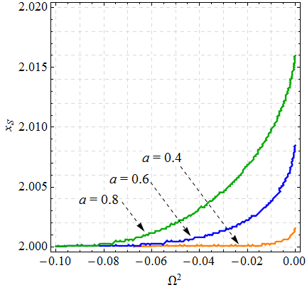
To solve Eq. (38), we use the shooting method described above for various values of , , and . Without loss of generality we put (thus fixing the length scale) and the initial value of the derivative, . The standard procedure of ODE solving leads to a numerical curve corresponding to a chosen test value of . This curve has a critical behavior with a drastically fluctuating sign at large at any non-eigenvalue . Tracking the value of allows us to “catch” the critical value of as a candidate for an eigenvalue with necessary accuracy. The result of such a numerical analysis is depicted in Fig. 2 for three values of . Each curve in this plot is actually a separatrix that separates regions of different signs of at large during the shooting procedure. The pairs along this separatrix, where up to a numerical error, correspond to solutions of the eigenvalue problem at fixed and indicate an instability of the system under consideration.
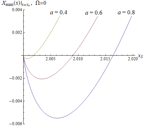
As is evident from Fig. 2 (left panel), the instability is only observed for inside quite a small interval , where . When , the corresponding eigenvalue . For each , the upper boundary can be found by numerically solving Eq. (38) with . In this case we obtain a curve that tends to some at large . This depends on and vanishes at some (see Fig. 2, right panel). For one can numerically find , respectively. These values of indicate the existence of a solution corresponding to the eigenvalue .
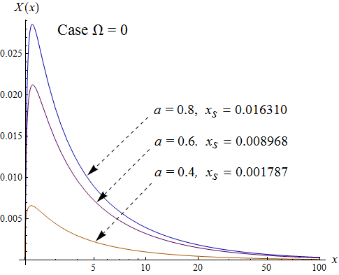
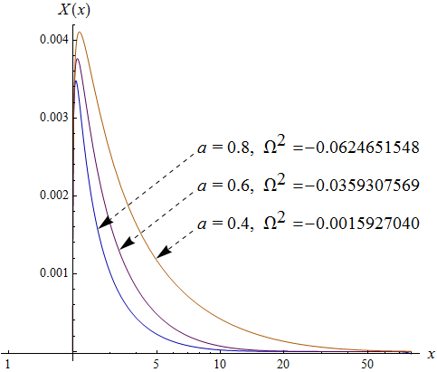
The eigenfunctions for different and are plotted in Fig. 3.
5.2 Boundary-value problem 2
An attempt to numerically solve Eq. (38) “from right to left,” specifying the boundary condition at large using Eq. (40) leads to a numerical instability near the singularity . Therefore, it makes sense to launch the “left to right” procedure, specifying the boundary condition close to , where a desired solution to Eq. (38) should tend to a constant value. In doing so, it is not possible to require simply and at some close to since quite evidently the last term in (38) proportional to blows up as and must create if not large then nonzero values of the derivative . To find suitable boundary conditions, let us find the asymptotic behavior of near in a better approximation than .
For convenience, let us rewrite Eq. (38) in terms of ,
| (41) | |||
| (42) |
and seek solutions at small in the form
| (43) |
The solutions are different for different values of :
- 1.
- 2.
. Then both terms with and behave as , and similarly to the previous case we obtain the constants
and the boundary conditions at , in the form
(45) - 3.
. Now the term with in Eq. (41) grows faster than as , and the latter can be neglected. Then in the same manner as before we obtain the constants
and the boundary conditions at ,
(46) One can notice that under these conditions the derivative is quite large at small , like that of the function near .
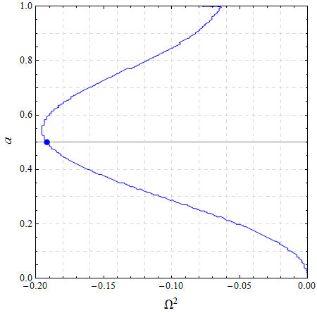
We implement the shooting method separately for each of the above three cases, putting and without loss of generality. We also put for suitable accuracy of the numerical plots. It is of interest to study the dependence of possible eigenvalues (if any) on the parameter . Using the method of tracking fluctuations of at large “right end” (as in the previous section), one can draw a corresponding separatrix, along which the pairs provide a solution to the eigenvalue problem.
The results of this analysis are depicted in Fig. 4 (left panel). One can see that despite the different nature of boundary conditions in cases 1–3 above, the resulting separatrix is continuous, including the particular point corresponding to the special case . This diagram allow us to draw a conclusion (at least up to the numerical accuracy governed by the choice of a small but finite starting value ) that there is an instability for all due to the existence of the eigenvalues . Examples of numerical solutions are shown in the right panel of Fig. 4.
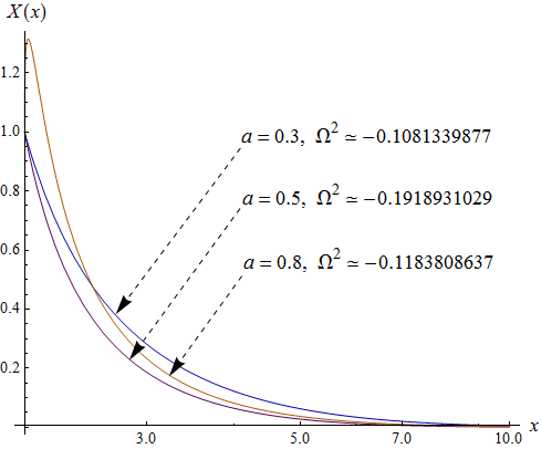
A note on the obtained increment values of unstable perturbations. In Fisher’s solution (2), the Schwarzschild mass is . The conformal factor changes this value, but generically does not change its order of magnitude, therefore, since is of the order of unity, we can say that in our STT solutions we also have . Therefore, with our scale fixing , the obtained values mean that the characteristic times of perturbation growth are approximately of the order of or slightly larger than the time needed for a photon to cover a distance , the gravitational radius of the corresponding Schwarzschild mass.
6 Conclusion
We have considered the linear stability problem for conformally Fisher space-times that comprise vacuum solutions of the Bergmann-Wagoner-Nordtvedt class of STT of gravity with massless scalar fields. Since the perturbation equations for these space-times, as a special case of gravitational-scalar field equations, formulated in the Jordan frame manifold , are transformed to the corresponding equations in , the latter, being common for all STT of the present class and coinciding with those of GR, acquire a universal meaning. Unlike that, the boundary conditions that select physically meaningful perturbations, depend on a particular STT and even on the properties of particular solution.
In some cases, the boundary conditions turn out to coincide with those already known in — in such cases the stability conclusions for also coincide with those for . In other cases, it is necessary to consider separate boundary value problems. This work has been done here for four well-know examples of STT, and its results are summarized in Table 1.
| Theory, solution | Description∗ | Results∗∗ |
| Brans-Dicke, | Singularity at , BVP 2 | unstable |
| Brans-Dicke, , | Singularity at , BVP 2 | unstable |
| Barker, | Singularity at , BVP 1 | stable |
| Barker, | Singularity at , BVP 1 | unstable |
| Schwinger, , | Singularity at , BVP 1 | stable |
| Schwinger, , | Singularity at , BVP 1 | unstable |
| Schwinger, , | Singularity at similar to Fisher’s | unstable + |
| Nonminimal coupling, , | Singularity at , BVP 2 | unstable |
| Nonminimal coupling, , | Singularity at , BVP 2 | unstable |
∗ BVP = boundary-value problem.
∗∗ “unstable” means that there is a perturbation mode with a finite increment ;
“unstable+” means that a perturbation increment is indefinite, as it is for Fisher’s solution.
It is clear that the present results are applicable to many more particular STT because the boundary-value problems 1 and 2 for spherical perturbations emerge under quite general conditions. In particular, it is true for various STT representations of various modified theories of gravity other than STT as such, for example, the original [26] and generalized [27] versions of hybrid metric-Palatini gravity, for which static, spherically symmetric solutions are discussed in [28, 29], as well as different models of nonlocal and high-order gravity, see, e.g., [30, 31, 32, 33].
Let us also recall that the present results have been obtained only for STT with massless scalars, while there are numerous models and solutions with nonzero scalar field potentials , see Eq. (1); note that theories of gravity are also reducible to STT with nonzero . Moreover, we have restricted ourselves to canonical (nonphantom) STT, whereas models with phantom scalars are also of much interest and even more diverse. In all cases, except for those with conformal continuations, it is possible to reduce the perturbation equations to those in the Einstein frame, but the appropriate boundary conditions must be formulated “individually” for each separate solution.
Funding
The research of K. Bronnikov, S. Bolokhov and M. Skvortsova was supported by RUDN University Project FSSF-2023-0003. K. Bronnikov was also supported by the Ministry of Science and Higher Education of the Russian Federation Project No. 0723-2020-0041. K. Badalov and R. Ibadov gratefully acknowledge the support from Ministry of Innovative Development of the Republic of Uzbekistan, Project No. FZ-20200929385.
References
- [1] K.A. Bronnikov and A.V. Khodunov. Scalar field and gravitational instability, Gen. Rel. Grav. 11, 13 (1979).
- [2] I. Z. Fisher, Scalar mesostatic field with regard for gravitational effects, J. Eksp. Teor. Fiz. 18, 636 (1948); gr-qc/9911008 (translation into English).
- [3] R.A. Konoplya and A. Zhidenko, Quasinormal modes of black holes: from astrophysics to string theory, Rev. Mod. Phys. 83, 793–836 (2011).
- [4] K. A. Bronnikov. Trapped ghosts as sources for wormholes and regular black holes. The stability problem. In: Wormholes, Warp Drives and Energy Conditions (Ed. F.S.N. Lobo, Springer, 2017), p. 137-160.
- [5] K.A. Bronnikov. Scalar fields as sources for wormholes and regular black holes, Particles 2018, 1, 5; arXiv: 1802.00098.
- [6] P.G. Bergmann, Comments on the scalar-tensor theory, Int. J. Theor. Phys. 1, 25 (1968).
- [7] R. Wagoner, Scalar-tensor theory and gravitational waves, Phys. Rev. D 1, 3209 (1970).
- [8] K. Nordtvedt, Post-Newtonian metric for a general class of scalar-tensor gravitational theories and observational consequences, Astroph. J. 161, 1059 (1970).
- [9] K.A. Bronnikov, Scalar-tensor theory and scalar charge, Acta Phys. Pol. B 4, 251 (1973).
- [10] K. A. Bronnikov, Scalar-tensor gravity and conformal continuations, J. Math. Phys. 43, 6096 (2002); gr-qc/0204001.
- [11] K.A. Bronnikov and A.A. Starobinsky, No realistic wormholes from ghost-free scalar-tensor phantom dark energy, Pis’ma v ZhETF 85, 1, 3-8 (2007); JETP Lett. 85, 1, 1-5 (2007).
- [12] K.A. Bronnikov, M.V. Skvortsova and A.A. Starobinsky, Notes on wormhole existence in scalar-tensor and F(R) gravity. Grav. Cosmol. 16, 216 (2010); arXiv: 1005.3262.
- [13] L.D. Landau and E.M. Lifshitz, Field Theory (Nauka, M., 1973).
- [14] O. Bergmann and R. Leipnik, Space-time structure of a static spherically symmetric scalar field, Phys. Rev. 107, 1157 (1957).
- [15] K. A. Bronnikov and S. G. Rubin. Black Holes, Cosmology, and Extra Dimensions (2nd edition, World Scientific, 2021).
- [16] C. Brans and R.H. Dicke, Mach’s principle and a relativistic theory of gravitation, Phys. Rev. 124 925 (1961).
- [17] B.M. Barker, General scalar-tensor theory of gravity with constant G, Astrophys. J. 219, 5 (1978).
- [18] J. Schwinger, Particles, Sources and Fields (Addison-Wesley, Reading, MA, Vol. 1, 1970).
- [19] William Bruckman, Generation of electro and magneto static solutions of the scalar-tensor theories of gravity , arXiv: gr-qc/9407003.
- [20] K.A. Bronnikov, Scalar vacuum structure in general relativity and alternative theories. Conformal continuations, Acta Phys. Pol. B 32, 3571 (2001); gr-qc/0110125.
- [21] K.A. Bronnikov, J.C. Fabris, and A. Zhidenko, On the stability of scalar-vacuum space-times, Eur. Phys. J. C 71, 1791 (2011).
- [22] N.M. Bocharova, K.A. Bronnikov and V.N. Melnikov, On an exact solution of the Einstein-scalar field equations. Vestnik MGU Fiz., Astron. No. 6, 706 (1970).
- [23] B. Liu, L. McLerran and N. Turok, Bubble nucleation and growth at a baryon-number-producing electroweak phase transition, Phys. Rev. D 46, 2668 (1992).
- [24] C. Barceló and M. Visser, Scalar fields, energy conditions, and traversable wormholes, Class. Quantum Grav. 17, 3843 (2000); gr-qc/0003025.
- [25] K.A. Bronnikov and S.V. Grinyok, Conformal continuations and wormhole instability in scalar-tensor gravity, Grav. Cosmol. 10, 237 (2004); gr-qc/0411063.
- [26] S. Capozziello, T.Harko, T. S. Koivisto, F. S. N. Lobo, and G. J. Olmo, Hybrid metric-Palatini gravity, Universe 1, 199 (2015); arXiv: 1508.04641.
- [27] C. G. Böhmer and N. Tamanini, Generalized hybrid metric-Palatini gravity, Phys. Rev. D 87, 084031 (2013); arXiv: 1302.2355.
- [28] K. A. Bronnikov, S. V. Bolokhov, and M. V. Skvortsova, Hybrid metric-Palatini gravity: Black holes, wormholes, singularities, and instabilities, Grav. Cosmol. 26 (3), 212-227 (2020).
- [29] K. A. Bronnikov, S. V. Bolokhov, and M. V. Skvortsova, Spherically symmetric space-times in generalized hybrid metric-Palatini gravity, Grav. Cosmol. 27 (4), 358-374 (2021).
- [30] S. Nojiri, S. D. Odintsov, and V. K. Oikonomou, Modified gravity theories in a nutshell: Inflation, bounce and late-time evolution, Phys. Rep. 692, 1-104 (2017); arXiv: 1705.11098.
- [31] S. Nojiri and S. D. Odintsov, Modified non-local-F(R) gravity as the key for the inflation and dark energy Phys. Lett. B 659, 821 (2008).
- [32] K. A. Bronnikov and E. Elizalde, Spherical systems in models of nonlocally corrected gravity, Phys. Rev. D 81, 044032 (2010).
- [33] S. V. Chervon, I. V. Fomin, and A. A. Chaadaev, Spherically symmetric solutions of a chiral self-gravitating model in gravity, Grav. Cosmol. 28 (3), 295-303 (2022).