An ML-assisted OTFS vs. OFDM adaptable modem

The next generation of wireless communications envisions a range of new applications like holographic communications, tactile internet, autonomous vehicles, robot swarms, UAVs, high-speed trains, and space communication to name a few. This calls for aggressive requirement specifications on the key performance indicators (KPI) for the next-generation wireless communication standards. For example, in 6G, some of the KPI specifications being considered include achieving peak data rates of 1 Tbps, with a reliability of 99.99999%, and having a network density of 10 million devices per square km. The air-interface latency being considered is 0.1 ms with dopplers up to 1000kmph [1, 2]. The combination of technologies like ultra-massive Multiple-Input Multiple-Output (uMaMIMO), reconfigurable Intelligent Surfaces (RIS), and terahertz communications is seen to be a key enabler in achieving such goals [3]. One of the important design considerations, particularly to support error-free communications at high dopplers is the choice of waveform and modulation scheme [2, 4]. It is known that, by designing the waveforms where the symbols are spread in the domain of selectivity, optimal performance can be achieved for perfect channel state information (CSI) assumption at the receivers [2]. Thus the Orthogonal-Frequency-Division-Multiplexing (OFDM) waveforms are susceptible to doubly-selective channel conditions that arise due to high mobility. On the other hand, the Orthogonal-Time-Frequency-Space (OTFS) waveforms spread the symbols both in time and frequency by placing them on a delay-doppler (DD) grid, ensuring that all the symbols experience “equal gain”, and hence are more amicable for high doppler scenarios [5, 2]. However, the OFDM waveform offers the advantage of having low-complexity receivers with simple channel equalization and detection capabilities.

In this section, we shall briefly review the OTFS system model and its relationship to OFDM [9]. The input-output (IO) relationship considering a linear MMSE combiner at the receiver is presented. The MSE expression for the OTFS and OFDM structures is derived using the IO relationship. The OTFS modulator places the information symbols $X_{dd}[k,l]$ along the DD grid of dimension $N\times M$ such that $k=0,1,\cdots,N-1$ and $l=0,1,\cdots,M-1$. The OTFS burst has a duration of $NT_{0}$ and occupies a bandwidth of $B=MF_{0}$, where $T_{0}$ and $F_{0}$ are the time and frequency resolution of the time-frequency (TF) plane of the burst under consideration such that $T_{0}F_{0}=1$. Hence the TF plane is characterized as $\Lambda=\Big\{(nT_{0},mF_{0}),n=0,1,\cdots,N-1,m=0,1,\cdots,M-1\Big\}$, and the DD plane as $\Gamma=\Big\{(\frac{k}{NT_{0}},\frac{l}{MF_{0}}),k=0,1,\cdots,N-1,l=0,1,\cdots,M-1\Big\}$. The terms $\nu_{0}=\frac{1}{NT_{0}}$ and $\tau_{0}=\frac{1}{MF_{0}}$ represent the doppler shift and the delay resolution of the DD plane [9]. An inverse symplectic finite Fourier transform (ISFFT) is performed to transform the symbols to TF representation $X_{tf}[n,m]$ which are later converted to time domain signals $s(t)$ using Heisenberg transform for transmission.

$g(t)$ is the unit-energy pulse of duration $T_{0}$. At the receiver, the received signal $r(t)$ that is corrupted by a doubly-selective channel with TF response $H(t,f)$ and AWGN noise $n(t)$ is transformed to TF representation $Y_{tf}[n,m]$ using Wigner transform, which is later converted back to DD domain using SFFT as $Y_{dd}[k,l]$ as shown in (2). The OTFS mod-demod (modem) architecture is shown in Fig 1.

Here $S(f)$ is the Fourier transform of $s(t)$. The TF response $H(t,f)$ of a doubly-dispersive channel can be written as

where $N_{p}$ is the number of multi-path components between the transmitter and the receiver, $\alpha_{k},\tau_{k}$, and $\nu_{k}$ represent the gain, delay, and doppler shift associated with the $k^{th}$ path, respectively. In the discrete form, we have $H_{tf}[n,m]=H(nT_{0},mF_{0})$. The complex baseband representation of the channel in the DD domain $H_{dd}[k,l]=H_{dd}(k\tau_{0},l\nu_{0})$ and the TF representation of the same $H_{tf}[n,m]$ are interchangeable using the SFFT/ISFFT.

In the proposed architecture, a binary ML classifier at the receiver observes the estimated TF channel $\hat{H}_{tf}[n,m]$, the estimate of the received SNR, and the QAM alphabet size to decide on the use of OTFS or OFDM waveforms in the current coherent interval. The modem operates in two modes, namely, training and realization modes, which are illustrated using Fig. 2. During the training phase of the modem, both OTFS and OFDM frames are transmitted within the same coherence time. There are many ways in which it can be accomplished. One possible design is to interleave the OFDM and OTFS frames. The receiver chains of the OFDM and the OTFS correspondingly extract the demodulated symbols $\mathbb{z}$ after channel estimation and equalization to compute the MSE $\delta_{\text{otfs}}$ and $\delta_{\text{ofdm}}$. The estimate of the actual TF channel $H_{tf}[n,m]$ is $\hat{H}_{tf}[n,m]$. A series of $p$ observations of the estimated channel $\hat{H}_{tf}[n,m]$, SNR $\rho$, QAM size $m$, and the resulting MSE $(\delta_{\text{otfs}},\delta_{\text{ofdm}})$ with the two waveforms are used to train the ML classifier. Once the ML is trained, the proposed architecture will be able to switch between the two waveforms seamlessly based on the channel conditions, SNR, and QAM size in the normal (realization) mode. The operation of the modem during the training and realization mode is depicted in Fig 2 and Fig 2, respectively.

During the ML training, a family of $p$ channels are generated with the configurations for the Extended Vehicular-A (EVA), Extended Pedestrian-A (EPA), and Extended Typical Urban (ETU) models defined in [12] using (3). These models have either seven or nine paths, and the delay profiles for each path are picked from a Gaussian distribution having a mean delay equal to the RMS delay, and with variance such that the path delay doesn’t exceed the maximum delay as specified in the standard [12]. The relative attenuation values for each of the paths are used directly from [12] and normalized to unity power. The Doppler shift associated with each of the paths is determined using $\nu_{i}=\nu_{max}cos(\theta_{i})$, where $\theta_{i}\in\mathcal{U}[0,\pi]$ [12]. For each of these channels, the MSE $\delta_{\text{otfs}}$ and $\delta_{\text{ofdm}}$ are evaluated at various SNRs $(\rho)\in\mathcal{S}$ and for different M-ary QAM symbols such that $M\in\mathcal{M}$. Here, we consider $\mathcal{S}=\{-20,-15,-10,-5,0,5,10,15,20,25,30\}$ dB, and $\mathcal{M}=\{4,16,64,256,1024\}$. Each of the channel $H_{tf}[n,m]$ obtained is corrupted such that ${\hat{H}_{tf}[n,m]}=H_{tf}[n,m]+\epsilon(\rho)$, where $\epsilon(\rho)$ is AWGN noise proportional to the received SNR. This simulates the channel estimation errors. This training data set is represented as $\mathcal{U}=\Big\{\{\hat{H}_{i}[n,m]\}_{i=1}^{p},\{\rho_{i}\}_{i=1}^{p},\{m_{i}\}_{i=1}^{p},\{w_{i}\}_{i=1}^{p}\Big\}$, Here $w_{i}\in\mathcal{W}=\{0,1\}$, with $0$ indicating OTFS and $1$ indicating OFDM, whichever yields the $min(\delta_{\text{otfs}},\delta_{\text{ofdm}})$.
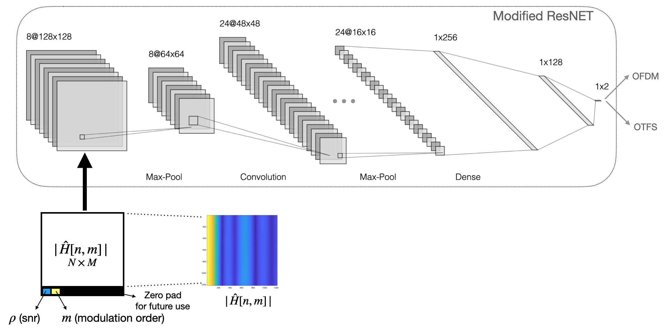
The training set $\mathcal{U}$ is then used to train a modified ResNET101 binary classifier [13]. The data set $\mathcal{U}$ is formatted as an image such that each TF channel $\hat{H}_{tf}[n,m]$ is converted into an image of size $(N+1)\times M$ with each pixel color intensity representative of $|\hat{H}_{tf}[n,m]|$. The additional row is zero-padded except for the two pixels that indicate the received SNR and the M-ary QAM size. This is depicted in the Fig. 4. To evaluate the realization mode of the modem post training, a test set of $q$ channels are generated using the models EVA, EPA, and ETU defined in [12] similar to $\mathcal{U}$ such that $\mathcal{U}\cap\mathcal{T}=\emptyset$. We choose $p=1000$ and $q=100$. The results obtained for a subset of the test configurations in $\mathcal{T}$ are shown in Fig. 3-3. It can be observed that the proposed architecture can switch between the two waveforms effectively in all the cases presented. The modified ResNET101 achieves a classification accuracy of $97.8$% with our simulations. Another general observation is that the OTFS performs better than OFDM in high Doppler scenarios with EVA models, irrespective of the modulation order, and at all SNRs. On the other hand, the OFDM performs better than OTFS at low to medium dopplers in ETV and ETU models with strong LOS and when multiple doppler shift paths are present for the same delay taps.

In this paper, an ML-assisted modem architecture to switch the signal processing chains within the transmitter and the receiver to enable either OTFS or OFDM waveforms is proposed. A modified ResNET101 binary classifier is trained to identify the switching criteria that depend on the channel conditions, received SNR, and QAM alphabet size to enhance the user experience in the MSE sense. This helps in unifying the advantages of both OTFS and OFDM schemes based on the operating conditions and for a given figure of merit (FoM), which is difficult to conclusively establish, as noted in previous literature and confirmed with our simulations. Using simulation, we also established that a well-trained ResNET101 binary classifier can seamlessly switch between these two waveforms to reduce the MSE at various operating conditions. Although MSE is used as the FoM in this work to elucidate the idea, one could choose other FoMs like throughput, capacity, energy efficiency, or computational complexity. Similarly, the switching criteria can be extended beyond channel conditions, received SNR, and QAM alphabet size to encompass other system parameters.

References

- [1] W. Tong and P. Zhu, 6G: The Next Horizon: From Connected People and Things to Connected Intelligence. Cambridge University Press, May 2021.
- [2] M. Chafii, L. Bariah, S. Muhaidat, and M. Debbah, “Twelve scientific challenges for 6g: Rethinking the foundations of communications theory,” IEEE Communications Surveys and Tutorials, vol. 25, no. 2, pp. 868–904, Feb 2023.
- [3] M. Alsabah, M. A. Naser, B. M. Mahmmod, S. H. Abdulhussain, M. R. Eissa, A. Al-Baidhani, N. K. Noordin, S. M. Sait, K. A. Al-Utaibi, and F. Hashim, “6g wireless communications networks: A comprehensive survey,” IEEE Access, vol. 9, pp. 148 191–148 243, 2021.
- [4] F. Conceição, M. Gomes, V. Silva, R. Dinis, A. Silva, and D. Castanheira, “A survey of candidate waveforms for beyond 5g systems,” Electronics, vol. 10, no. 1, Dec 2020.
- [5] R. Hadani, S. Rakib, M. Tsatsanis, A. Monk, A. J. Goldsmith, A. F. Molisch, and R. Calderbank, “Orthogonal time frequency space modulation,” 2017 IEEE Wireless Communications and Networking Conference (WCNC), pp. 1–6, March 2017.
- [6] C. D’Andrea, S. Buzzi, M. Fresia, and X. Wu, “Doppler-resilient universal filtered multicarrier (dr-ufmc): A beyond-otfs modulation,” Feb 2023.
- [7] L. Gaudio, G. Colavolpe, and G. Caire, “Otfs vs. ofdm in the presence of sparsity: A fair comparison,” IEEE Transactions on Wireless Communications, vol. 21, no. 6, pp. 4410–4423, June 2022.
- [8] G. P. Fettweis and H. Boche, “6g: The personal tactile internet—and open questions for information theory,” IEEE BITS the Information Theory Magazine, vol. 1, no. 1, pp. 71–82, Sep 2021.
- [9] P. Raviteja, K. T. Phan, Q. Jin, Y. Hong, and E. Viterbo, “Low-complexity iterative detection for orthogonal time frequency space modulation,” 2018 IEEE Wireless Communications and Networking Conference (WCNC), pp. 1–6, April 2018.
- [10] A. M. Sayeed, “How is time frequency space modulation related to short time fourier signaling?” 2021 IEEE Global Communications Conference (GLOBECOM), pp. 1–6, Dec 2021.
- [11] S. K. Mohammed, R. Hadani, A. Chockalingam, and R. Calderbank, “Otfs—a mathematical foundation for communication and radar sensing in the delay-doppler domain,” IEEE BITS the Information Theory Magazine, vol. 2, no. 2, pp. 36–55, Nov 2022.
- [12] ETSI, “Evolved universal terrestrial radio access (e-utra); user equipment (ue) radio transmission and reception,” 3GPP TS 36.101 Release 14, vol. 14.3.0, no. 101, pp. 1282–1283, April 2017.
- [13] K. He, X. Zhang, S. Ren, and J. Sun, “Deep residual learning for image recognition,” 2016 IEEE Conference on Computer Vision and Pattern Recognition (CVPR), pp. 770–778, June 2016.