Transition probabilities of near-infrared Ce III lines from stellar spectra: applications to kilonovae
Abstract
Kilonova spectra provide us with information of -process nucleosynthesis in neutron star mergers. However, it is still challenging to identify individual elements in the spectra mainly due to lack of experimentally accurate atomic data for heavy elements in the near-infrared wavelengths. Recently, Domoto et al. 2022 proposed the absorption features around 14500 Å in the observed spectra of GW170817/AT2017gfo as Ce III lines. But they used theoretical transition probabilities (-values) whose accuracy is uncertain. In this paper, we derive the astrophysical -values of the three Ce III lines, aiming at verification of this identification. We model high resolution -band spectra of four F-type supergiants showing the clear Ce III absorption features by assuming stellar parameters derived from optical spectra in literatures. We also test the validity of the derived astrophysical -values by estimating Ce III abundances in Ap stars. We find that the derived astrophysical -values of the Ce III lines are systematically lower by about 0.25 dex than those used in previous work of kilonovae, while they are still compatible within the uncertainty range. By performing radiative transfer simulations of kilonovae with the derived -values, we find that the identification of Ce III as a source of the absorption features in the observed kilonova spectra still stands, even considering the uncertainties in the astrophysical -values. This supports identification of Ce in the spectra of GW170817/AT2017gfo.
Keywords:
line: identification — stars: neutron — stars: general — atomic dataI Introduction
Binary neutron star (NS) mergers have been considered as promising sites of -process nucleosynthesis (Eichler et al. 1989; Freiburghaus et al. 1999; Goriely et al. 2011; Korobkin et al. 2012; Wanajo et al. 2014, e.g.,). In 2017, associated with the detection of gravitational waves (GWs) from a NS merger (Abbott et al. 2017a, GW170817,), the electromagnetic counterpart AT2017gfo was observed (Abbott et al. 2017b). The observed properties of AT2017gfo in ultraviolet, optical, and near-infrared (NIR) wavelengths are consistent with the theoretical expectation of a kilonova (Li & Paczyński 1998; Metzger et al. 2010), thermal emission from NS merger ejecta powered by radioactive decays of -process nuclei (Arcavi et al. 2017; Evans et al. 2017; Pian et al. 2017; Smartt et al. 2017; Utsumi et al. 2017; Valenti et al. 2017, e.g.,). This electromagnetic counterpart has provided us with evidence that NS mergers are sites of -process nucleosynthesis (Kasen et al. 2017; Perego et al. 2017; Shibata et al. 2017; Tanaka et al. 2017; Kawaguchi et al. 2018; Rosswog et al. 2018, e.g.,).
To extract the detailed information of elements synthesized in NS merger ejecta, it is important to identify the individual elements. However, element identification in the kilonova spectra remains challenging. This is mainly due to lack of atomic data for heavy elements. While detailed spectral studies require spectroscopically accurate atomic data, such data for heavy elements have been highly incomplete, especially for the NIR wavelengths. So far, the absorption features around 8000 Å in the photospheric spectra of AT2017gfo have been identified as Sr II (Watson et al. 2019; Domoto et al. 2021; Gillanders et al. 2022), although the same features may be caused by He I (Perego et al. 2017; Tarumi et al. 2023).
Recently, Domoto et al. 2022 systematically studied kilonova spectra over the entire wavelength range. They identified important elements that produce strong transitions in kilonvoae, such as Ca, Sr, Y, Zr, Ba, La, and Ce. Then, they constructed a hybrid line list combined with experimentally accurate data for important elements and complete theoretical data for weak transitions of the other elements (Tanaka et al. 2020). By performing radiative transfer simulations, they found that the broad line features at 13000 Å and 14500 Å in the spectra of AT2017gfo can be explained by La III and Ce III, respectively. However, this identification can be still a subject of discussion as they adopted the transition probabilities (i.e., -values) of the La III and Ce III lines from theoretical calculations (Tanaka et al. 2020) due to lack of experimental measurements.
The lack of experimental atomic data is problematic in any spectra for astrophysical objects, such as stars. Compared with the optical region, line identification in stellar spectra in the NIR region is incomplete and still in progress (Matsunaga et al. 2020, e.g.,). Also, as few experiments have been performed on heavy elements such as lanthanides, -values from theoretical calculations are commonly used even for the optical wavelengths. In many cases, no or few data are provided for the NIR wavelengths (Biémont et al. 1999; Quinet & Palmeri 2020, e.g.,).
In general, the accuracy of atomic calculations is difficult to assess without experimental measurements. It has been shown that the theoretical -values for given ions differ from the experimental values several times for strong transitions, and even more for weak transitions (Domoto et al. 2022, see, e.g., Appendix of). The -values directly affect the absorption depths in the spectra, which influences derived parameters, e.g., abundances. In the case of kilonova model of Domoto et al. 2022, the absorption features at the NIR wavelengths can disappear if the -values of the NIR lines are times smaller than the values they adopted. Therefore, it is important to measure the -values to firmly identify elements in kilonova spectra.
For the use in astrophysics, one can estimate the -values of atomic lines by using stellar spectra. This is often called as “astrophysical -values”. Such work has been performed for many metal lines in the NIR wavelengths using the spectra of well-observed stars, e.g., the Sun (Meléndez & Barbuy 1999, e.g.,). In fact, it has been shown that the astrophysical -values can be useful to extract elemental information from stars without laboratory experiments (Hasselquist et al. 2016; Cunha et al. 2017).
In this paper, we derive the astrophysical -values of three Ce III lines at the -band (around 1.6 µm) using high resolution stellar spectra. This aims to verify the identification of Ce in the spectra of AT2017gfo. Note that we cannot test the absorption by La III in the same way, because the La III lines at rest lie in the wavelength region of strong atmospheric absorption. In Section II, we describe the targeted Ce III lines in more detail. We present the stellar spectra showing the Ce III line features in Section III, and derive the -values of the Ce III lines by modeling these spectra in Section IV. In Section V, we apply the derived -values of the Ce III lines to kilonova spectra by performing radiative transfer simulations. Finally, we give a summary in Section VI. We also show the validity of our results by estimating the Ce abundances with Ce III lines in Ap stars in Appendix A. Throughout of the paper, line wavelengths are written as those in vacuum unless otherwise mentioned.
| a | b | c | d | Theoretical log | Astrophysical log | ||||||
|---|---|---|---|---|---|---|---|---|---|---|---|
| (Å) | (Å) | () | () | (1) | (2) | (3) | (4) | (5) | (6) | (7) | This work |
| 15851.880 | 15847.550 | 1528.32 | 7836.72 | 0.613 | 0.838 | 1.030 | 1.190 | 0.439 | 0.673 | 2.105 | 0.861 |
| 15961.157 | 15956.797 | 0.00 | 6265.21 | 0.721 | 0.926 | 1.120 | 1.290 | 2.926 | 1.098 | 0.345 | 0.966 |
| 16133.170 | 16128.763 | 3127.10 | 9325.51 | 0.509 | 0.722 | 0.920 | 1.070 | 0.429 | 1.950 | 0.920 | 0.702 |
Note. — a Vacuum transition wavelength.
b Air transition wavelength.
c Lower energy level.
d Upper energy level.
e -values from theoretical calculations (1: Tanaka et al. 2020, see also Domoto et al. 2022; 2: Wyart & Palmeri 1998; 3: taken from Hubrig et al. 2012 and Chojnowski et al. 2019. These values were computed in the same way as in Biémont et al. 2002 and provided to Hubrig et al. 2012 and Chojnowski et al. 2019 as private communication; 4: Carvajal Gallego et al. 2021). For (1) and (4), theoretical -values are shown as they are, without calibration by considering the differences in the theoretical energy levels relative to the experimental energy levels.
f Astrophysical -values in the APOGEE line list (5: Shetrone et al. 2015, Table 7 of; 6: taken from here through the SDSS Science Archival Server (SAS), see Holtzman et al. 2018; 7: taken from here through the SDSS SAS, see Smith et al. 2021), and those derived in this work (Section IV).
II Ce III lines at -band
We focus on the three Ce III lines at the -band (Table 1). It has been shown that these are the strongest lines of Ce III in the NIR region, which can produce broad absorption features in kilonova spectra (Domoto et al. 2022). In fact, these lines have been detected in the spectra of Ap/Bp stars that exhibit enhanced Ce abundances (Hubrig et al. 2012; Chojnowski et al. 2019; Tanaka et al. 2023).
Although the transition wavelengths of these lines have been measured by experiments (Johansson & Litzén 1972), their transition probabilities are experimentally unknown. Thus, Domoto et al. 2022 adopted the theoretical results of Tanaka et al. 2020. Other theoretical calculations are also available, i.e., used for studies of optical stellar spectra (Wyart & Palmeri 1998; Biémont et al. 2002) and for application to kilonovae (Carvajal Gallego et al. 2021). However, it is usually difficult to assess the accuracy of these calculations, and the -values vary over the range of dex as shown in Table 1.
Recently, the APOGEE survey has observed many Galactic stars at the -band with the spectral resolution of (Majewski et al. 2017). To analyze the APOGEE spectra, the line lists for the -band have been provided (Shetrone et al. 2015; Holtzman et al. 2018; Smith et al. 2021). They collected the atomic data from theoretical and experimental studies, and adjusted the -values by fitting those to the spectra of the Sun and Arcturus. It is shown that such astrophysical -values can improve the agreement between the observed spectra and the model spectra. In fact, the APOGEE line lists include the three Ce III lines that we focus on (Table 1). However, their astrophysical -values are quite uncertain, because there is no clear Ce III absorption in the spectra of the Sun and Arcturus. As a result, the -values vary by an order of magnitude across the different versions of the APOGEE line lists. This fact demonstrates that, if lines are not clearly detected in the spectra which is the case of Ce III lines for the Sun and Arcturus, it is difficult to derive the astrophysical -values even though the spectra are well characterized. To derive -values of the Ce III lines, we select stars clearly showing these Ce III line features (Section III), although the uncertainties in stellar parameters can be larger than those of well-known stars such as the Sun and Arcturus (Section IV.3).
We mention that near the three lines, there is another Ce III line at 15964.93 Å. According to the theoretical -values of this line (1.272 by Tanaka et al. 2020, 1.660 by Biemont et al., see Chojnowski et al. 2019, or 1.690 by Carvajal Gallego et al. 2021), this line is weaker than the three Ce III lines. In fact, it is found that the absorption at this wavelength is usually dominated by the strong Si I 15964.41 Å line (see Figure 1). Thus, we will not focus on this line in this work.

III Stellar spectra with Ce III lines
III.1 Sample selection
Compared with the NIR wavelengths, the line list in the optical region is more comprehensive and accurate. Ce abundances in many stars are indeed reported from optical observations, e.g., in Hypatia Catalog for Solar neighborhoods (Hinkel et al. 2014), the catalogue of luminous stars (Luck 2014), and the catalogue of chemically peculiar (CP) stars (Ghazaryan et al. 2018). While not all the stars in these catalogues have Ce abundances, measurements are available for a good fraction of stars. Thus, we will derive the astrophysical -values of the Ce III lines using the stars that (1) show the Ce III line features in the NIR -band and (2) have known Ce abundances from optical spectra.
We obtain NIR -band high resolution spectra from the spectral archive of the Immersion GRating INfrared Spectrometer (Park et al. 2014; Mace et al. 2016; Mace et al. 2018, IGRINS,). IGRINS provides spectra spanning the full and bands with the spectral resolution of . The Raw & Reduced IGRINS Spectral Archive (RRISA)11 1 https://igrinscontact.github.io/ contains the IGRINS archive for the period of July 2014–December 2021 on the 2.7 m Harlan J. Smith Telescope at McDonald Observatory, the Discovery Channel Telescope at Lowell Observatory, and the Gemini south telescope. RRISA includes IGRINS data from more than 850 nights on-sky, resulting in 2800 unique target observations from over 3000 hours of the total science time. RRISA also includes the IGRINS observations of distinct A0V standard stars.
RRISA provides reduced one-dimensional (1D) spectra processed using the IGRINS pipeline (Lee et al. 2017). The pipeline applies flat-fielding and flagging of bad pixels, and the 1D spectra are extracted using the optimal extraction of Horne 1986. The wavelength solutions are derived using OH lines from sky spectra. In the -band, the accuracy of wavelength solution is better than 0.01 Å ( 0.2 km s-1). RRISA further refines the wavelength of the pipeline product by improving the pixel alignment between the A0V star spectrum and the target spectrum using strong telluric sky lines between 16452–16458 Å and 21740–21752 Å in the - and -band, respectively. Telluric absorption is corrected using the spectra of A0V stars observed closely in time and airmass with intrinsic features of A0V stars removed using a model spectrum of the Vega (Castelli & Kurucz 1994).
We crossmatch the RRISA archive with the two stellar catalogues of measured abundances: Luck 2014 and Ghazaryan et al. 2018. Not all entries in these catalogues have Ce abundances reported, and they are not used as we need abundance information to derive the -values (see below). Luck 2014 reports abundances for 451 luminous stars including Ce measurement for 448 stars. RRISA contains spectra for 27 of them. Ghazaryan et al. 2018 reports abundances of 429 CP stars with 121 stars of Ce measurement. RRISA contains spectra of 8 stars.
For the matched data, we apply Doppler correction using strong C I, Si I, and Fe I lines. Then, we visually check the absorption lines at the wavelengths of the Ce III lines. We impose the detection of all three lines to ensure the origin of these lines. As a result, six stars showing clear Ce III line features are selected: HD 29647, HD 56126, Cas, Aql, HD 190323, and d Dra. The spectra of six stars around the regions of the Ce III lines are shown in Figure 1.
While the six stars are selected above, we decide not to use two out of them: HD 29647 and HD 56126 (gray lines in Figure 1). This is because their atmospheric parameters are found to be rather uncertain, although they are listed in the catalogues. For HD 29647, a HgMn star (Straizys et al. 1985), Adelman et al. 2001 have reported the atmospheric parameters, but they mentioned that the parameters are not very accurate. For HD 56126, a post-AGB star (Hony et al. 2003, e.g.,), atmospheric parameters seem to change depending on the epoch when spectra are taken (De Smedt et al. 2016; Puķītis et al. 2022). Puķītis et al. 2022 also pointed out the chemical depletion of neutron-capture elements in other post-AGB star, likely due to dust condensation. Also, the IGRINS spectrum of HD 56126 shows double-peak like features, whose origins are unknown.
Finally, we use four stars as our samples (black lines in Figure 1). The S/N ratios of the spectra around the targeted Ce III lines are for Aql and for the others. Since the Ce III 15851.88 Å and 16133.170 Å lines are located around the broad hydrogen features, the spectra are normalized by fitting the broad features as a pseudo-continuum. After the normalization, we measure the equivalent widths (EWs) of the Ce III lines by Gaussian fitting (see the top panels of Figure 3 as examples). The measured EWs of the Ce III lines in each star are shown in Table 3, which are used to derive those astrophysical -values in Section IV.
| Star | Spectral type | Model | log | [Fe/H] | [Al/H] | [Si/H] | [Ce/H] | a | |||
|---|---|---|---|---|---|---|---|---|---|---|---|
| (K) | (cm s-2) | (km s-1) | (km s-1) | ||||||||
| Cas | F0Ia | ATLAS | 7347 | 0.76 | 0.07 | 5.21 | 23.0∗ | 0.00b | 0.49 | 0.16 | 0.30 |
| Aql | F2Ib | ATLAS | 7152 | 1.65 | 0.10 | 3.74 | 12.0∗∗ | 0.22 | 0.32 | 0.27 | 0.22 |
| HD 190323 | F8Ia | MARCS | 6169 | 1.11 | 0.12 | 4.31 | 15.0‡ | 0.42 | 0.27 | 0.25 | 0.15 |
| d Dra | F8Ib-2 | MARCS | 6157 | 1.78 | 0.10 | 3.93 | 10.0† | 0.16 | 0.06 | 0.27 | 0.24 |
Note. — All the parameters are adopted from Luck 2014, but from Abt & Morrell 1995 (∗), Uesugi & Fukuda 1970 (∗∗), Lyubimkov et al. 2012 (†), and estimated in this work using the Ce III line because of no available measurement (‡).
a Standard deviations of the Ce abundances measured in Luck 2014 (see Section IV.3).
b The solar abundance (Asplund et al. 2009) is assumed because it is not measured in Luck 2014.
III.2 Properties of sample stars
The four stars in our final sample are all F-type supergiants (see Table 2). Our primary catalogue of Luck 2014 consists primarily of (super)giants with 4000–8000 K, and the Ce III lines are only seen in warmer supergiants of K. To check the presence of the Ce III lines in wider parameter range of and surface gravity log , we also crossmatch the RRISA with Hinkel et al. 2014. RRISA contains spectra of 132 sources out of 2685 stars from Hinkel et al. 2014, primarily of nearby dwarf stars. But none of the spectra show clear signature of the Ce III lines. We further check RRSIA with and log from the PASTEL catalogue (Soubiran et al. 2016). RRISA contains spectra of 168 stars with –8000 K, mostly dwarfs with some (super)giants. Note that this catalogue does not provide abundance measurements and is not subject to our analysis of deriving the -values. We find five stars showing the Ce III line features, which are the same four stars as our sample selected from Luck 2014 and an additional F-type supergiant.
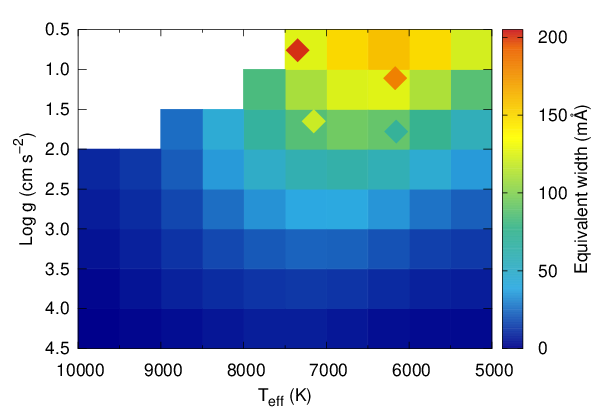
We briefly discuss the reason why the Ce III lines tend to appear in warm supergiants. To see the behavior of the Ce III absorption in spectra, we generate model spectra for the wavelength regions around the Ce III lines, varying and log . We use Turbospectrum (Plez 2012) implemented through iSpec (Blanco-Cuaresma et al. 2014; Blanco-Cuaresma 2019) to perform spectral synthesis, assuming local thermodynamic equilibrium (LTE). The parameter ranges are = 5000–10000 K and log = 0.5–4.5 dex with intervals of 500 K and 0.5 dex, respectively. For simplicity, we fix the microturbulent velocity = 2 km s-1, the solar abundance ratio (Asplund et al. 2009), and the projected rotational velocity = 10 km s-1as typical values (Matsunaga et al. 2020, e.g.,), and assume the macroturbulent velocity km s-1(see also Section IV.1). We use ATLAS, 1D plane-parallel atmosphere model (Castelli & Kurucz 2003). For the atomic data, we use the APOGEE line list (Holtzman et al. 2018; Smith et al. 2021, see Section IV.1) as a baseline, with the line list of the Ce III lines from Domoto et al. 2022. These choices do not affect the dependence on and log discussed here.
Since the dependence of the absorption on the atmospheric parameters is expected to be the same among the Ce III lines, we focus only on the Ce III 15961.157 Å line. Note that this Ce III line may be contaminated by Al I 15961.03 Å line at lower and higher log , although the Ce III line is dominant (Section IV.1). We measure the EWs of the Ce III line in the model spectra by Gaussian fitting as done in the observed spectra. The measured EWs for different and log are shown in Figure 2. It is seen that the EW of the Ce III line peaks at 6000–7000 K and log 2. The peak can be understood as the region where the doubly ionized Ce is the most abundant under LTE. Also, the line becomes strong toward low gravity, due to low-density and geometrically thick atmosphere (Gray 2005). A similar trend is observed for other lines of metal ions (Matsunaga et al. 2020).
We also show the observed EWs of the Ce III 15961.157 Å line for the four sample stars as shown with diamonds in Figure 2. Although the Ce abundances are not exactly same as the solar abundances for these stars, it is seen that the observed trend is consistent with the trend in our model grid. Also, models are consistent with the fact that only warm (F-type) supergiants show the Ce III lines but not normal dwarfs.
Of course, the behavior of the Ce III lines are also dependent on the Ce abundance. If the Ce abundance is higher, the parameter range of and log showing the Ce III lines becomes wider. For example, as shown in Figure 1, HD 29647 shows Ce III absorption in the NIR wavelengths even under high temperature and strong surface gravity (Adelman et al. 2001, K and log ,), because the Ce abundance is dex higher than the solar value (see also Appendix A). We note that CP stars are main sequences; supergiants used in our analysis do not show such anomaly in abundances of lanthanides.

IV Astrophysical -values of the Ce III lines
IV.1 Methods
In this section, we derive the astrophysical -values of the Ce III lines. For each sample star, we perform spectral synthesis calculations with the fixed Ce abundances based on the measurements with the optical spectra, and then adjust -values. We use Turbospectrum (Plez 2012) through iSpec (Blanco-Cuaresma et al. 2014; Blanco-Cuaresma 2019) to synthesize spectra as in Section III.2.
We adopt atmospheric parameters (, log , metallicity, and ) derived from the analysis of optical spectra. Luck 2014 provided the stellar parameters of sample stars using MARCS models (Gustafsson et al. 2008). For the stars with higher than K, they also used ATLAS models (Castelli & Kurucz 2003). In our sample, when a star has two parameter sets determined using both models, we use the atmospheric parameters that better reproduce the -band IGRINS spectra. Then, for spectral synthesis, we consistently use MARCS or ATLAS models used in the estimates of the adopted atmospheric parameters. The adopted atmospheric parameters and models of sample stars are summarized in Table 2.
We use the elemental abundances derived using the adopted atmospheric parameters in Luck 2014. Luck 2014 used observational data from multiple archives and provided abundances for each of the available data for a given star. When multiple abundance sets are provided for our sample stars, we simply take the averages. While all the elements are included in our calculations, only Ce, Al, and Si are important for our analysis: Ce abundances directly affect the absorption depths of the Ce III lines, while Al and Si may also affect the Ce III absorption due to the contamination by Al I 15961.03 Å and Si I 16133.42 Å lines, respectively. For the elements without measurements, we assume the solar abundances (Asplund et al. 2009). For example, the Al abundance for Cas is assumed as the solar abundance. But this assumption does not affect the results because most Al is expected to be ionized in a high ( K) and low log ( dex) atmosphere (see also Section IV.3 and Table 4). For all the samples, the contamination from the Al I and Si I lines for the Ce III absorption features are estimated to be % and %, respectively, by measuring the EWs of the lines in the model spectra without the Ce III lines. The adopted abundances of important elements are also summarized in Table 2.
It should be cautioned that, although the Ce abundances are fixed in our analysis, they are also subject to the uncertainties (see also Section IV.3). The standard deviations of the Ce abundances measured in Luck 2014 are also shown in Table 2. We confirmed that the absorption of Ce II lines at the -band (Cunha et al. 2017) is reasonably reproduced for HD 190323 and d Dra, which confirms the validity of the abundances. There is no or little Ce II absorption for Cas and Aql with K. Nevertheless, we emphasize that the Ce abundances in these two stars are rather robust, because they were derived using optical lines with experimental -values (Luck 2014).
Spectral synthesis also needs to consider effects of line broadening. It is usually difficult to separate the effects of and on the line profiles in F-type supergiants (Lyubimkov et al. 2012, e.g.,). Here, we ignore and consider only . These parameters for Cas, Aql, and d Dra are taken from literatures (see Table 2). We find that these choices reasonably reproduce the line profiles in the IGRINS spectra. On the other hand, no measurement of for HD 190323 was found. Thus, we estimate using the Ce III lines in the IGRINS spectra (see Table 2). Although this is not very accurate measurement, this assumption does not affect our results.
The line list for other elements is also an important factor in the estimate of -values. This is because some Ce III lines are contaminated by Al I or Si I lines. Thus, the -values of these lines may affect the estimates of the -values of the Ce III lines. By comparing the -band model spectra using the VALD (Piskunov et al. 1995; Kupka et al. 1999; Ryabchikova et al. 2015) and the APOGEE line lists (Holtzman et al. 2018; Smith et al. 2021), we find that the APOGEE line list reproduces the observed features of the IGRINS spectra better. Thus, we adopt the APOGEE line list for our analysis. Note that, as iSpec implements the APOGEE line list of DR13/14 (Holtzman et al. 2018), we updated the line list using the newest DR16 line list (Smith et al. 2021) except for hyperfine structure lines.
For the model spectra, we measure the EWs of the Ce III lines by Gaussian fitting as done in the observed spectra. These EWs are compared with those of the observed spectra (Section III.1). Comparison is repeated by changing the -values of the Ce III lines. Finally, we adopt the -values that give the EWs in agreement with the EWs of the observed spectra. Examples of the final model spectra are shown in the bottom panels of Figure 3.

| Star | EW (mÅ) | log | EW (mÅ) | log | EW (mÅ) | log |
|---|---|---|---|---|---|---|
| 15851.880 Å | 15961.157 Å | 16133.170 Å | ||||
| Cas | 184 | 0.82 | 201 | 0.80 | 166 | 0.72 |
| Aql | 102 | 0.93 | 120 | 0.96 | 96 | 0.83 |
| HD 190323 | 183 | 0.78 | 182 | 0.90 | 180 | 0.65 |
| d Dra | 81 | 0.92 | 71 | 1.20 | 113 | 0.61 |
| Star | log | [Fe/H] | [Al/H] | [Si/H] | ||||
|---|---|---|---|---|---|---|---|---|
| (Å) | (+200 K) | (+0.3 dex) | (+0.3 dex) | (+0.5 km s-1) | (+0.5 dex) | (+0.3 dex) | ||
| Cas | 15851.880 | 0.146 | 0.067 | 0.035 | 0.018 | - | - | 0.165 |
| 15961.157 | 0.105 | 0.085 | 0.029 | 0.030 | 0.002 | - | 0.141 | |
| 16133.170 | 0.139 | 0.070 | 0.034 | 0.010 | - | 0.022 | 0.161 | |
| Aql | 15851.880 | 0.048 | 0.153 | 0.028 | 0.017 | - | - | 0.164 |
| 15961.157 | 0.054 | 0.151 | 0.025 | 0.019 | 0.015 | - | 0.164 | |
| 16133.170 | 0.067 | 0.151 | 0.046 | 0.014 | - | 0.088 | 0.193 | |
| HD 190323 | 15851.880 | 0.000 | 0.176 | 0.066 | 0.030 | - | - | 0.190 |
| 15961.157 | 0.003 | 0.179 | 0.057 | 0.021 | 0.031 | - | 0.192 | |
| 16133.170 | 0.018 | 0.175 | 0.100 | 0.026 | - | 0.099 | 0.227 | |
| d Dra | 15851.880 | 0.015 | 0.196 | 0.055 | 0.011 | - | - | 0.204 |
| 15961.157 | 0.002 | 0.194 | 0.056 | 0.005 | 0.121 | - | 0.235 | |
| 16133.170 | 0.014 | 0.194 | 0.081 | 0.014 | - | 0.149 | 0.258 |
IV.2 Results
The estimated -values of the three Ce III lines using the spectra of four stars are shown by blue dots in Figure 4, and listed in Table 3. As our final astrophysical -values of each Ce III line, we take the averages of those derived for each star. They are plotted as red dots in each panel of Figure 4, and listed in Table 1. The validity of our final -values is also discussed in Appendix A.
The -values of the Ce III lines from available theoretical calculations are also shown by black diamonds in Figure 4 (see Table 1). All of our -values are consistently smaller than those of Tanaka et al. 2020, which were used for the kilonova model of Domoto et al. 2022. This suggests that the strength of absorption could have been overestimated in the kilonova model of Domoto et al. 2022 (see Section V). On the other hand, it is seen that the estimated final -values are the closest to those of Wyart & Palmeri 1998, while higher than those of Biémont et al. 2002 and Carvajal Gallego et al. 2021. Overall, our -values of the Ce III lines, which are independently estimated from theoretical calculations, broadly agree with the available theoretical calculations within the margin of the estimated uncertainties discussed in Section IV.3.
IV.3 Uncertainties in -values
Uncertainties in the astrophysical -values can be evaluated by considering the uncertainties in the stellar parameters of each star. The systematic uncertainty of stellar parameters can generally be caused by difference in the analysis methods. Even with common atmospheric parameters and line lists, there remain variety in the abundances determined by different codes and methods (Hinkel et al. 2016) as well as different spectral data used in the analysis (Luck 2014). All of these factors can affect the depth of absorption lines, which leads to uncertainties in the astrophysical -values derived for the fixed Ce abundances.
We estimate the systematic uncertainties in our astrophysical -values by varying stellar parameters of each star. To take uncertainties of stellar parameters into account, we vary by 200 K, log by 0.3 dex, [Fe/H] by 0.3 dex, and by 0.5 km s-1. Also, we vary [Al/H] and [Si/H] by 0.5 and 0.3 dex, respectively, which affect the level of the contamination. These ranges are typical systematic uncertainties caused by different codes and methods used to determine stellar parameters (Hinkel et al. 2016). While Hinkel et al. 2016 used dwarfs to show these uncertainty ranges, the uncertainties for supergiants are similar to those in dwarfs (Luck 2014).
Table 4 summarizes the estimated systematic uncertainties in the astrophysical -values of the Ce III lines. Only the results for the positive shifts are shown, but the results for the negative shifts are smaller than the uncertainties given in Table 4 (Cunha et al. 2017, see also Table 3 of ). We find that the largest uncertainties are caused by or log . The systematic uncertainties in total in each -value for each star () are estimated by taking root sum squares (Cunha et al. 2017). Note that the values of estimated here are the upper limits of the uncertainties: all the stellar parameters are not independent, and the uncertainties caused by each parameter may be cancelled among parameters (Cunha et al. 2017). In most cases, the total systematic uncertainties are smaller than 0.2 dex, and up to dex. These systematic uncertainties are shown as the error bars for the blue dots in Figure 4.
Finally, we assign the systematic uncertainties of the average astrophysical -values by taking root mean squares of the in four stars. The systematic uncertainties in the -values for 15851.880 Å, 15961.157 Å, and 16133.170 Å lines are 0.182, 0.186, and 0.213, respectively (shown as the error bars for the red dots in Figure 4). It is worth noting that our astrophysical -values are broadly agree with available theoretical calculations, considering the systematic uncertainties.
Here we did not show the uncertainties in continuum levels of the observed spectra in . They may affect the observed EWs and in turn astrophysical -values. However, the uncertainties in continuum leveles and their contributions to are estimated to be 1%, which are smaller than the uncertainties from most stellar parameters (Cunha et al. 2017, see also Table 3 of).
Note that, although we fix the Ce abundances of each star to derive astrophysical -values, the Ce abundances are still uncertain within the range of dex (standard deviations, Section IV.1). The Ce abundances scale the resultant -values: for example, if the Ce abundance is altered by the standard deviation (Table 2) to the positive direction, the derived -values are also affected by the same degree to the negative direction. Furthermore, it should be noted that the Ce abundances in Luck 2014 as well as the astrophysical -values here were derived under the assumption of LTE. Non-LTE treatment may affect the abundances of heavy elements (Mashonkina et al. 2005, e.g.,), especially in supergiants. This may result in systematic changes in the derived -values. Nevertheless, the fact that the derived -values are consistent among samples suggests that the Ce abundance of each star adopted in this work is reasonable. Independent measurements of stellar parameters may be able to reduce the uncertainties in the astrophysical -values, but this is beyond the scope of this work. The uncertainties present here are found not to significantly affect the final results on kilonova spectra, as discussed in Section V.


V Applications to kilonova spectra
We apply the derived -values of the Ce III lines to calculate kilonova spectra. To calculate synthetic spectra of kilonovae, we use a wavelength-dependent radiative transfer simulation code (Tanaka & Hotokezaka 2013; Tanaka et al. 2014; Tanaka et al. 2017; Tanaka et al. 2018; Kawaguchi et al. 2018; Kawaguchi et al. 2020). The photon transfer is calculated by the Monte Carlo method. The setup of simulation is identical to that in Domoto et al. 2022, but we adopt the final astrophysical -values of the three Ce III lines derived in Section IV. For more details of the simulation, we refer the readers to Domoto et al. 2022.
Figure 5 shows the comparison between our new synthetic spectra (blue) and the observed spectra of AT2017gfo taken with the Very Large Telescope (VLT) (gray) at , 2.5, and 3.5 days after the merger (Pian et al. 2017; Smartt et al. 2017). The observed spectra at days after the merger taken with the Hubble Space Telescope (HST), which are not affected by telluric absorption, is also shown by a black line (Tanvir et al. 2017). We find that the absorption features around 14500 Å are caused by the Ce III lines in the new spectra. These features are blueshifted according to the velocity of the line-forming region at the NIR wavelengths, e.g., at days. In fact, the features caused by the Ce III lines in the new synthetic spectra are almost the same as those in Domoto et al. 2022, which used the -values of Tanaka et al. 2020 (see Figure 6 for the enlarged view at days). This is consistent with the observed features in the spectra of AT2017gfo.
To see the effects of the uncertainties in the -values to the spectra, we also perform the same simulations by varying the -values of the Ce III lines. Orange and red curves in Figure 6 show the results when using the lower and upper -values, respectively. Here, for the lower (upper) values, we take the averages of the estimated -values for each star negatively (positively) shifed by , and then further shift the averages by negatively (positively). We find that the changes in fluxes around 14500 Å are %. The absorption features by Ce III are still seen even using the lower -values (orange curves), although the depth of absorption is weakened.
When using the final astrophysical -values, the Sobolev optical depths of the Ce III lines for the line forming region ( g cm-3 and K, see Domoto et al. 2022) are . The lower -values of the Ce III lines are smaller than the nominal values by a factor of . Thus, even by adopting the lower -values, the Sobolev optical depths of the Ce III lines are still larger 1. This confirms the identification of Ce in the spectra of AT2017gfo.
The changes in -values of the strong lines affect not only absorption but also emission in the spectra. A stronger absorption tends to cause a stronger emission in P-Cygni type line profile. As shown in Figure 6, the increase of the -values results in the increase of the flux at emission component around the rest wavelengths, and vice versa. Note that, for particularly large -values (red and green lines), the optical depths of the Ce III lines are large enough that the depth of the absorption is saturated, while the effect in the emission component is still apparent.
VI Summary
We have derived the astrophysical -values of the three Ce III lines at the -band using the IGRINS spectra of four F-type supergiants. The derived -values are systematically lower by about 0.25 dex than those used in Domoto et al. 2022, but they are broadly agree with available theoretical calculations within the estimated uncertainties. Using the derived astrophysical -values of the Ce III lines, we have performed radiative transfer simulations of kilonovae. We have found that the Ce III lines with the new -values produce the absorption features around 14500 Å in kilonova spectra, even considering the uncertainties. This supports the identification of Ce in the observed spectra of AT2017gfo (Domoto et al. 2022).
We have also shown that the F-type supergiants with near solar metallicity show strong absorption of Ce III. To our knowledge, this is the first report of the detection of the Ce III lines at the -band in stars with near solar abundances. As the line blending is not severe in the NIR spectra compared with the optical spectra, those lines may also be useful for stellar spectroscopic studies.
Appendix A Abundance estimates in Ap stars as a test of astrophysical -values
We assess the validity of our astrophysical -values by adopting them to spectra of Ap stars. Ap stars are a kind of CP stars that exhibit extremely high metal abundances. Thanks to the high abundances, Ap stars show clear Ce III absorption lines that we focus on. However, it is also known that they show inconsistent abundances between singly and doubly ionized rare-earth elements (REE), called REE anomaly (Ryabchikova et al. 2004; Ryabchikova & Romanovskaya 2017). Even if Ce abundances have been measured from Ce II lines, it does not necessarily represent the Ce abundances. Therefore, these stars cannot be used to derive -values in Section IV.
Here, we estimate the Ce abundances from Ce III lines (hereafter Ce III abundances) in Ap stars using the derived astrophysical -values. We use three Ap stars, HD 101065 (Przybylski’s Star), HD 201601 ( Equ), and HD 24712. These stars have quite different log from the supergiants used to derive the -values. Thus, the abundance estimates serve as independent assessment of the derived -values.
The spectrum of HD 101065 was taken with Gemini south/IGRINS on UT 2022 December 18 in two ABBA sequences with each exposure time of 33 sec. An A0V star (HIP 55019) was also observed for the telluric standard. Those IGRINS spectra are reduced through the pipeline (Lee et al. 2017), as described in Section III.1. The 1D spectra are normalized by continuum fitting.
The spectra of HD 201601 and HD 24712 were taken with the Gemini Near-Infrared Spectrograph (Elias et al. 2006a; Elias et al. 2006b, GNIRS,) at Gemini north telescope on UT 2022 July 17 and August 18, respectively. We use 110.5 l/mm grating and long camera with a 0.1” slit, which gives the spectral resolution of 17800. Central wavelength is set to be 1.6 µm to cover the three Ce III lines. HD 201601 and HD 24712 were observed in one and two ABBA sequence(s) with each exposure time of 60 sec, respectively. For the telluric standards, A0V stars (HD 208108 and HD 15130) were also observed. The GNIRS spectra are reduced using the Gemini IRAF package, and followed standard procedure, which includes flat-fielding, sky subtraction, wavelength calibration based on Ar-Xe lamp spectra, and extraction of 1D spectra. The 1D spectra are normalized by continuum fitting. Telluric absorption in the normalized target spectra is corrected by dividing by the normalized spectra of the A0V stars.
The spectra of three Ap stars around the region of the Ce III lines are show in Figure 7. For those spectra, we measure EWs of the three Ce III lines by Gaussian fitting. Then, we perform spectral synthesis as in Section IV but by changing the Ce abundance and by using the derived -values of the Ce III lines. We use the stellar parameters of the Ap stars derived in literatures using optical spectra as summarized in Table 5. Although there are the atmospheric parameters derived using more sophisticated models that consider stratification of elements for all the samples (Shulyak et al. 2009; Shulyak et al. 2010; Shulyak et al. 2013), we adopt those derived using 1D atmospheric models (ATLAS) that we use for spectral synthesis. We measure EWs of the Ce III lines in model spectra by Gaussian fitting and compare with the EWs in the observed spectra. Comparison is repeated by varying Ce abundances until the model EWs match with the EWs in the observed spectra.
We show the results of the Ce III abundances estimated using the three Ce III lines in Table 6. It is seen that the line-by-line variation of the abundances is small in each star. This fact demonstrates that the derived -values of the Ce III lines are reasonable.
Table 6 also shows the Ce II and III abundances reported in literatures, which confirms clear REE anomaly. It is worth noting that, although Hubrig et al. 2012 showed that the derived Ce III abundances in HD 201601 deviate about 2 dex depending on the lines, the abundances derived by using the three Ce III lines here are consistent with each other. Also, this is the first measurement of the Ce III abundance for HD 24712.

| Star | Model | log | [Fe/H] | [Al/H] | [Si/H] | Reference | |||
|---|---|---|---|---|---|---|---|---|---|
| (K) | (cm s-2) | (km s-1) | (km s-1) | ||||||
| HD 101065 | ATLAS | 6600 | 4.20 | 0.72 | 1.00 | 3.5 | 1.11 | 0.11 | Cowley et al. 2000 |
| HD 201601 | ATLAS | 7700 | 4.20 | 0.19 | 2.00 | 7.0a | 0.66 | 0.11 | Ryabchikova et al. 1997a |
| HD 24712 | ATLAS | 7250 | 4.20 | 0.21 | 1.00 | 6.6a | 0.06 | 0.18 | Ryabchikova et al. 1997b |
Note. — All are smaller than spectral resolution ( or 17800) and does not affect results.
a Adopted from Sikora et al. 2019.
| [Ce/H] | HD 101065 | HD 201601 | HD 24712 | |
|---|---|---|---|---|
| Ce III | 15851.880 Å | 4.11 | 4.09 | 3.86 |
| 15961.157 Å | 4.06 | 4.04 | 3.72 | |
| 16133.170 Å | 4.16 | 4.26 | 3.83 | |
| Mean standard error | 4.110.03 | 4.130.07 | 3.780.03 | |
| Literatures | 4.76a | 3.46–5.36c | ||
| Ce II | 2.93a | 1.26d | 1.42e | |
| 3.07b |
Note. — a Shulyak et al. 2010. b Cowley et al. 2000. c Hubrig et al. 2012. d Ryabchikova et al. 1997a. e Ryabchikova et al. 1997b.
References
- Abbott et al. (2017a) Abbott, B. P., Abbott, R., Abbott, T. D., et al. 2017a, Phys. Rev. Lett., 119, 161101, doi: 10.1103/PhysRevLett.119.161101
- Abbott et al. (2017b) —. 2017b, ApJ, 848, L12, doi: 10.3847/2041-8213/aa91c9
- Abt & Morrell (1995) Abt, H. A., & Morrell, N. I. 1995, ApJS, 99, 135, doi: 10.1086/192182
- Adelman et al. (2001) Adelman, S. J., Snow, T. P., Wood, E. L., et al. 2001, MNRAS, 328, 1144, doi: 10.1046/j.1365-8711.2001.04936.x
- Arcavi et al. (2017) Arcavi, I., Hosseinzadeh, G., Howell, D. A., et al. 2017, Nature, 551, 64, doi: 10.1038/nature24291
- Asplund et al. (2009) Asplund, M., Grevesse, N., Sauval, A. J., & Scott, P. 2009, ARA&A, 47, 481, doi: 10.1146/annurev.astro.46.060407.145222
- Biémont et al. (1999) Biémont, E., Palmeri, P., & Quinet, P. 1999, Ap&SS, 269, 635, doi: 10.1023/A:1017049314691
- Biémont et al. (2002) Biémont, E., Quinet, P., & Ryabchikova, T. A. 2002, MNRAS, 336, 1155, doi: 10.1046/j.1365-8711.2002.05868.x
- Blanco-Cuaresma (2019) Blanco-Cuaresma, S. 2019, MNRAS, 486, 2075, doi: 10.1093/mnras/stz549
- Blanco-Cuaresma et al. (2014) Blanco-Cuaresma, S., Soubiran, C., Heiter, U., & Jofré, P. 2014, A&A, 569, A111, doi: 10.1051/0004-6361/201423945
- Carvajal Gallego et al. (2021) Carvajal Gallego, H., Palmeri, P., & Quinet, P. 2021, MNRAS, 501, 1440, doi: 10.1093/mnras/staa3729
- Castelli & Kurucz (1994) Castelli, F., & Kurucz, R. L. 1994, A&A, 281, 817
- Castelli & Kurucz (2003) Castelli, F., & Kurucz, R. L. 2003, in Modelling of Stellar Atmospheres, ed. N. Piskunov, W. W. Weiss, & D. F. Gray, Vol. 210, A20, doi: 10.48550/arXiv.astro-ph/0405087
- Chojnowski et al. (2019) Chojnowski, S. D., Hubrig, S., Hasselquist, S., et al. 2019, ApJ, 873, L5, doi: 10.3847/2041-8213/ab0750
- Cowley et al. (2000) Cowley, C. R., Ryabchikova, T., Kupka, F., et al. 2000, MNRAS, 317, 299, doi: 10.1046/j.1365-8711.2000.03578.x
- Cunha et al. (2017) Cunha, K., Smith, V. V., Hasselquist, S., et al. 2017, ApJ, 844, 145, doi: 10.3847/1538-4357/aa7beb
- De Smedt et al. (2016) De Smedt, K., Van Winckel, H., Kamath, D., et al. 2016, A&A, 587, A6, doi: 10.1051/0004-6361/201527430
- Domoto et al. (2022) Domoto, N., Tanaka, M., Kato, D., et al. 2022, ApJ, 939, 8, doi: 10.3847/1538-4357/ac8c36
- Domoto et al. (2021) Domoto, N., Tanaka, M., Wanajo, S., & Kawaguchi, K. 2021, ApJ, 913, 26, doi: 10.3847/1538-4357/abf358
- Eichler et al. (1989) Eichler, D., Livio, M., Piran, T., & Schramm, D. N. 1989, Nature, 340, 126, doi: 10.1038/340126a0
- Elias et al. (2006a) Elias, J. H., Joyce, R. R., Liang, M., et al. 2006a, in Society of Photo-Optical Instrumentation Engineers (SPIE) Conference Series, Vol. 6269, Ground-based and Airborne Instrumentation for Astronomy, ed. I. S. McLean & M. Iye, 62694C, doi: 10.1117/12.671817
- Elias et al. (2006b) Elias, J. H., Rodgers, B., Joyce, R. R., et al. 2006b, in Society of Photo-Optical Instrumentation Engineers (SPIE) Conference Series, Vol. 6269, Ground-based and Airborne Instrumentation for Astronomy, ed. I. S. McLean & M. Iye, 626914, doi: 10.1117/12.671765
- Evans et al. (2017) Evans, P. A., Cenko, S. B., Kennea, J. A., et al. 2017, Science, 358, 1565, doi: 10.1126/science.aap9580
- Freiburghaus et al. (1999) Freiburghaus, C., Rosswog, S., & Thielemann, F. K. 1999, ApJ, 525, L121, doi: 10.1086/312343
- Ghazaryan et al. (2018) Ghazaryan, S., Alecian, G., & Hakobyan, A. A. 2018, MNRAS, 480, 2953, doi: 10.1093/mnras/sty1912
- Gillanders et al. (2022) Gillanders, J. H., Smartt, S. J., Sim, S. A., Bauswein, A., & Goriely, S. 2022, MNRAS, 515, 631, doi: 10.1093/mnras/stac1258
- Goriely et al. (2011) Goriely, S., Bauswein, A., & Janka, H.-T. 2011, ApJ, 738, L32, doi: 10.1088/2041-8205/738/2/L32
- Gray (2005) Gray, D. F. 2005, The Observation and Analysis of Stellar Photospheres (Cambridge University Press), doi: 10.1017/cbo9781316036570
- Gustafsson et al. (2008) Gustafsson, B., Edvardsson, B., Eriksson, K., et al. 2008, A&A, 486, 951, doi: 10.1051/0004-6361:200809724
- Hasselquist et al. (2016) Hasselquist, S., Shetrone, M., Cunha, K., et al. 2016, ApJ, 833, 81, doi: 10.3847/1538-4357/833/1/81
- Hinkel et al. (2014) Hinkel, N. R., Timmes, F. X., Young, P. A., Pagano, M. D., & Turnbull, M. C. 2014, AJ, 148, 54, doi: 10.1088/0004-6256/148/3/54
- Hinkel et al. (2016) Hinkel, N. R., Young, P. A., Pagano, M. D., et al. 2016, ApJS, 226, 4, doi: 10.3847/0067-0049/226/1/4
- Holtzman et al. (2018) Holtzman, J. A., Hasselquist, S., Shetrone, M., et al. 2018, AJ, 156, 125, doi: 10.3847/1538-3881/aad4f9
- Hony et al. (2003) Hony, S., Tielens, A. G. G. M., Waters, L. B. F. M., & de Koter, A. 2003, A&A, 402, 211, doi: 10.1051/0004-6361:20030240
- Horne (1986) Horne, K. 1986, PASP, 98, 609, doi: 10.1086/131801
- Hubrig et al. (2012) Hubrig, S., Castelli, F., González, J. F., et al. 2012, A&A, 542, A31, doi: 10.1051/0004-6361/201218968
- Johansson & Litzén (1972) Johansson, S., & Litzén, U. 1972, Phys. Scr, 6, 139, doi: 10.1088/0031-8949/6/2-3/007
- Kasen et al. (2017) Kasen, D., Metzger, B., Barnes, J., Quataert, E., & Ramirez-Ruiz, E. 2017, Nature, 551, 80, doi: 10.1038/nature24453
- Kawaguchi et al. (2018) Kawaguchi, K., Shibata, M., & Tanaka, M. 2018, ApJ, 865, L21, doi: 10.3847/2041-8213/aade02
- Kawaguchi et al. (2020) —. 2020, ApJ, 889, 171, doi: 10.3847/1538-4357/ab61f6
- Korobkin et al. (2012) Korobkin, O., Rosswog, S., Arcones, A., & Winteler, C. 2012, MNRAS, 426, 1940, doi: 10.1111/j.1365-2966.2012.21859.x
- Kupka et al. (1999) Kupka, F., Piskunov, N., Ryabchikova, T. A., Stempels, H. C., & Weiss, W. W. 1999, A&AS, 138, 119, doi: 10.1051/aas:1999267
- Lee et al. (2017) Lee, J.-J., Gullikson, K., & Kaplan, K. 2017, Igrins/Plp 2.2.0, Zenodo, Zenodo, doi: 10.5281/zenodo.845059
- Li & Paczyński (1998) Li, L.-X., & Paczyński, B. 1998, ApJ, 507, L59, doi: 10.1086/311680
- Luck (2014) Luck, R. E. 2014, AJ, 147, 137, doi: 10.1088/0004-6256/147/6/137
- Lyubimkov et al. (2012) Lyubimkov, L. S., Lambert, D. L., Kaminsky, B. M., et al. 2012, MNRAS, 427, 11, doi: 10.1111/j.1365-2966.2012.21617.x
- Mace et al. (2016) Mace, G., Kim, H., Jaffe, D. T., et al. 2016, in Society of Photo-Optical Instrumentation Engineers (SPIE) Conference Series, Vol. 9908, Ground-based and Airborne Instrumentation for Astronomy VI, ed. C. J. Evans, L. Simard, & H. Takami, 99080C, doi: 10.1117/12.2232780
- Mace et al. (2018) Mace, G., Sokal, K., Lee, J.-J., et al. 2018, in Society of Photo-Optical Instrumentation Engineers (SPIE) Conference Series, Vol. 10702, Ground-based and Airborne Instrumentation for Astronomy VII, ed. C. J. Evans, L. Simard, & H. Takami, 107020Q, doi: 10.1117/12.2312345
- Majewski et al. (2017) Majewski, S. R., Schiavon, R. P., Frinchaboy, P. M., et al. 2017, AJ, 154, 94, doi: 10.3847/1538-3881/aa784d
- Mashonkina et al. (2005) Mashonkina, L., Ryabchikova, T., & Ryabtsev, A. 2005, A&A, 441, 309, doi: 10.1051/0004-6361:20053085
- Matsunaga et al. (2020) Matsunaga, N., Taniguchi, D., Jian, M., et al. 2020, ApJS, 246, 10, doi: 10.3847/1538-4365/ab5c25
- Meléndez & Barbuy (1999) Meléndez, J., & Barbuy, B. 1999, ApJS, 124, 527, doi: 10.1086/313261
- Metzger et al. (2010) Metzger, B. D., Martínez-Pinedo, G., Darbha, S., et al. 2010, MNRAS, 406, 2650, doi: 10.1111/j.1365-2966.2010.16864.x
- Park et al. (2014) Park, C., Jaffe, D. T., Yuk, I.-S., et al. 2014, in Society of Photo-Optical Instrumentation Engineers (SPIE) Conference Series, Vol. 9147, Ground-based and Airborne Instrumentation for Astronomy V, ed. S. K. Ramsay, I. S. McLean, & H. Takami, 91471D, doi: 10.1117/12.2056431
- Perego et al. (2017) Perego, A., Radice, D., & Bernuzzi, S. 2017, ApJ, 850, L37, doi: 10.3847/2041-8213/aa9ab9
- Pian et al. (2017) Pian, E., D’Avanzo, P., Benetti, S., et al. 2017, Nature, 551, 67, doi: 10.1038/nature24298
- Piskunov et al. (1995) Piskunov, N. E., Kupka, F., Ryabchikova, T. A., Weiss, W. W., & Jeffery, C. S. 1995, A&AS, 112, 525
- Plez (2012) Plez, B. 2012, Turbospectrum: Code for spectral synthesis, Astrophysics Source Code Library, record ascl:1205.004. http://ascl.net/1205.004
- Puķītis et al. (2022) Puķītis, K., Začs, L., & Grankina, A. 2022, ApJ, 928, 29, doi: 10.3847/1538-4357/ac4bc8
- Quinet & Palmeri (2020) Quinet, P., & Palmeri, P. 2020, Atoms, 8, 18, doi: 10.3390/atoms8020018
- Rosswog et al. (2018) Rosswog, S., Sollerman, J., Feindt, U., et al. 2018, A&A, 615, A132, doi: 10.1051/0004-6361/201732117
- Ryabchikova et al. (2004) Ryabchikova, T., Nesvacil, N., Weiss, W. W., Kochukhov, O., & Stütz, C. 2004, A&A, 423, 705, doi: 10.1051/0004-6361:20041012
- Ryabchikova et al. (2015) Ryabchikova, T., Piskunov, N., Kurucz, R. L., et al. 2015, Phys. Scr, 90, 054005, doi: 10.1088/0031-8949/90/5/054005
- Ryabchikova et al. (1997a) Ryabchikova, T. A., Adelman, S. J., Weiss, W. W., & Kuschnig, R. 1997a, A&A, 322, 234
- Ryabchikova et al. (1997b) Ryabchikova, T. A., Landstreet, J. D., Gelbmann, M. J., et al. 1997b, A&A, 327, 1137
- Ryabchikova & Romanovskaya (2017) Ryabchikova, T. A., & Romanovskaya, A. M. 2017, Astronomy Letters, 43, 252, doi: 10.1134/S1063773717040065
- Shetrone et al. (2015) Shetrone, M., Bizyaev, D., Lawler, J. E., et al. 2015, ApJS, 221, 24, doi: 10.1088/0067-0049/221/2/24
- Shibata et al. (2017) Shibata, M., Fujibayashi, S., Hotokezaka, K., et al. 2017, Phys. Rev. D, 96, 123012, doi: 10.1103/PhysRevD.96.123012
- Shulyak et al. (2010) Shulyak, D., Ryabchikova, T., Kildiyarova, R., & Kochukhov, O. 2010, A&A, 520, A88, doi: 10.1051/0004-6361/200913750
- Shulyak et al. (2013) Shulyak, D., Ryabchikova, T., & Kochukhov, O. 2013, A&A, 551, A14, doi: 10.1051/0004-6361/201220425
- Shulyak et al. (2009) Shulyak, D., Ryabchikova, T., Mashonkina, L., & Kochukhov, O. 2009, A&A, 499, 879, doi: 10.1051/0004-6361/200911623
- Sikora et al. (2019) Sikora, J., Wade, G. A., Power, J., & Neiner, C. 2019, MNRAS, 483, 2300, doi: 10.1093/mnras/sty3105
- Smartt et al. (2017) Smartt, S. J., Chen, T. W., Jerkstrand, A., et al. 2017, Nature, 551, 75, doi: 10.1038/nature24303
- Smith et al. (2021) Smith, V. V., Bizyaev, D., Cunha, K., et al. 2021, AJ, 161, 254, doi: 10.3847/1538-3881/abefdc
- Soubiran et al. (2016) Soubiran, C., Le Campion, J.-F., Brouillet, N., & Chemin, L. 2016, A&A, 591, A118, doi: 10.1051/0004-6361/201628497
- Straizys et al. (1985) Straizys, V., Cernis, K., & Hayes, D. S. 1985, Ap&SS, 112, 251, doi: 10.1007/BF00653507
- Tanaka & Hotokezaka (2013) Tanaka, M., & Hotokezaka, K. 2013, ApJ, 775, 113, doi: 10.1088/0004-637X/775/2/113
- Tanaka et al. (2014) Tanaka, M., Hotokezaka, K., Kyutoku, K., et al. 2014, ApJ, 780, 31, doi: 10.1088/0004-637X/780/1/31
- Tanaka et al. (2020) Tanaka, M., Kato, D., Gaigalas, G., & Kawaguchi, K. 2020, MNRAS, 496, 1369, doi: 10.1093/mnras/staa1576
- Tanaka et al. (2017) Tanaka, M., Utsumi, Y., Mazzali, P. A., et al. 2017, PASJ, 69, 102, doi: 10.1093/pasj/psx121
- Tanaka et al. (2018) Tanaka, M., Kato, D., Gaigalas, G., et al. 2018, ApJ, 852, 109, doi: 10.3847/1538-4357/aaa0cb
- Tanaka et al. (2023) Tanaka, M., Domoto, N., Aoki, W., et al. 2023, ApJ, 953, 17, doi: 10.3847/1538-4357/acdc95
- Tanvir et al. (2017) Tanvir, N. R., Levan, A. J., González-Fernández, C., et al. 2017, ApJ, 848, L27, doi: 10.3847/2041-8213/aa90b6
- Tarumi et al. (2023) Tarumi, Y., Hotokezaka, K., Domoto, N., & Tanaka, M. 2023, arXiv e-prints, arXiv:2302.13061, doi: 10.48550/arXiv.2302.13061
- Uesugi & Fukuda (1970) Uesugi, A., & Fukuda, I. 1970, Catalogue of rotational velocities of the stars (Faculty of Science, Kyoto University)
- Utsumi et al. (2017) Utsumi, Y., Tanaka, M., Tominaga, N., et al. 2017, PASJ, 69, 101, doi: 10.1093/pasj/psx118
- Valenti et al. (2017) Valenti, S., Sand, D. J., Yang, S., et al. 2017, ApJ, 848, L24, doi: 10.3847/2041-8213/aa8edf
- Wanajo et al. (2014) Wanajo, S., Sekiguchi, Y., Nishimura, N., et al. 2014, ApJ, 789, L39, doi: 10.1088/2041-8205/789/2/L39
- Watson et al. (2019) Watson, D., Hansen, C. J., Selsing, J., et al. 2019, Nature, 574, 497, doi: 10.1038/s41586-019-1676-3
- Wyart & Palmeri (1998) Wyart, J.-F., & Palmeri, P. 1998, Phys. Scr, 58, 368, doi: 10.1088/0031-8949/58/4/013