Photon noise correlations in millimeter-wave telescopes
Abstract
Many modern millimeter and submillimeter (“mm-wave”) telescopes for astronomy are deploying more detectors by increasing detector pixel density, and with the rise of lithographed detector architectures and high-throughput readout techniques, it is becoming increasingly practical to overfill the focal plane. However, when the pixel pitch is small compared to the product of the wavelength and the focal ratio , or , the Bose term of the photon noise correlates between neighboring detector pixels due to the Hanbury Brown & Twiss (HBT) effect. When this HBT effect is non-negligible, the array-averaged sensitivity scales with detector count less favorably than the uncorrelated limit of . In this paper, we present a general prescription to calculate this HBT correlation based on a quantum optics formalism and extend it to polarization-sensitive detectors. We then estimate the impact of HBT correlations on the sensitivity of a model mm-wave telescope and discuss the implications for focal-plane design.
1 Introduction
Modern millimeter and submillimeter (“mm-wave”) telescopes for astronomy are often limited by fluctuations in the background radiation. This is especially true for ground-based experiments where emission from the atmosphere and telescope are substantial. At high frequencies (e.g., optical wavelengths), the mode’s mean occupation number , and photon fluctuations are dominated by uncorrelated shot noise such that . At low frequencies (e.g., radio wavelengths), and photon fluctuations are dominated by the Bose term of the photon noise (“wave noise”) which correlates such that . Millimeter wavelengths lie in a cross-over regime where , making the calculation of array-averaged sensitivity in general nontrivial.
In addition, many modern mm-wave telescopes, particularly those equipped with cryogenic bolometric detector arrays, are field-of-view-limited and therefore aim to increase detector count by increasing pixel density, which is typically cheaper than building more telescopes. In this high-pixel-density paradigm, it is possible to overfill the focal plane such that neighboring detectors sample the same spatial mode. As we will show, this mode sharing introduces photon-noise correlations when the pixel spacing , where is the effective focal ratio at the focal plane and is the operational wavelength of interest. In this oversampled regime, photon noise correlations can have substantial impacts on the array-averaged sensitivity.
The theory of intensity correlations from incoherent sources has been studied extensively Fano 1961; Glauber 1963a; Glauber 1963b; Mandel and Wolf 1963; Carter and Wolf 1975; Carter and Wolf 1977, and the phenomenon was experimentally demonstrated by Hanbury Brown and Twiss (HBT) via measurements of the angular diameter of distant astronomical sources Brown et al. 1952; Brown and Twiss 1954; Brown and Twiss 1956. The impact of HBT correlations on mm-wave telescopes is discussed by Padin Padin 2010, where an empirical factor is introduced in an attempt to account for the corresponding sensitivity degradation.
In this paper, we present a prescription to estimate HBT correlations among detectors in millimeter- or submillimeter-wave telescopes based on a quantum optics formalism adopted from a circuit-based formalism for thermal photon correlations in quantum detectors developed by Zmuidzinas Zmuidzinas 2003. We then extend this formalism to polarization-sensitive detectors and use it to calculate the impact of HBT correlations on the sensitivity of a model mm-wave telescope.
This paper is organized as follows. In Sec. 2, we review the theoretical foundations of our formalism based on Ref. Zmuidzinas 2003 and show how they relate to the HBT effect Brown et al. 1952; Brown and Twiss 1954; Brown and Twiss 1956 and the van Cittert-Zernike theorem (VCZT) van Cittert 1934; Zernike 1938. We also show the formalism’s relation to the standard single-detector sensitivity calculations for a bolometer (e.g., see Ref. Hill et al. 2018 and references therein). Section 3 defines a model optical system for estimating the array-averaged sensitivity impact of HBT correlations. In Sec. 4, we derive an expression for the intensity correlation using this model optical system. Section 5 discusses the impact of HBT correlations on the sensitivity of a telescope system with close-packed detectors on the focal plane. In Sec. 6, we discuss the implications of the presented sensitivity optimization for the design of mm-wave detector arrays. Finally, Sec. 7 presents our conclusions.
2 Theoretical foundations
In this section, we review the theory of photon-count statistics and reformulate them to the context of astronomical telescope systems. We first adopt the treatment of thermal photon correlations derived by Zmuidzinas Zmuidzinas 2003, which uses the machinery of transmission lines and scattering matrices to calculate the propagation of quantum modes in a linear optical system. We then apply this treatment to optical systems, where the optical equivalence theorem Sudarshan 1963 allows us to equate the scattering matrix for quantum modes with the mode-mode coupling of classical waves (e.g., those obtained via physical optics calculations). We then show a few simple examples that relate this formalism to the the HBT effect, VCZT, and photon-noise calculations.
2.1 Photon correlations
We first consider a linear, lossy network of input ports detected at an output port .11 1 There is no fundamental distinction between the inputs and outputs, and every port has both incoming and outgoing photons, even though we will relate the input ports to optical input and the output ports to detectors. Input modes enter the network along semi-infinite transmission lines via the photon creation operator and are mapped onto the outputs via the scattering matrix . Loss in the system is modeled by an orthogonal scattering matrix , which governs the noise added between input mode and output mode . Given this structure (Fig. 1), the creation operator at output and mode frequency is
| (1) |
As demonstrated in Eq. (1), there is no fundamental distinction between the input/output ports and the lossy ports. Therefore, for simplicity, we hereafter absorb the scattering matrix for the lossy ports into and treat both mechanisms via a single unified scattering matrix.
The two-photon expectation value at detector outputs and is given by
| (2) |
Here, the expectation values are taken over quantum-statistical mixed states, governed by the density matrix, and represent the quantum coherence of the photon modes at frequencies and . See Appendix A for further discussion regarding the thermal photon density matrix.
When the mixed states are in thermal equilibrium, which is a good approximation for the photon sources in the calculations that follow Zmuidzinas 200322 2 The Kronecker delta in Eq. (3) indicates complete incoherence between the input source elements and . This is a good approximation for the applications discussed in this paper. Further discussion on partial coherence of sources can be found in Appendix B.,
| (3) |
where is the temperature of port and
| (4) |
is the mean occupation number at frequency of a blackbody at temperature . We can write the two-photon output expectation value as
| (5) |
where is the quantum mutual intensity and satisfies
| (6) |
When calculated for a single detector , represents the mean occupation number of the incoming photons at that detector.
Thermal detectors, which are commonly used in mm-wave applications, integrate photon power over time and sense mean intensity
| (7) |
where we define the time-dependent operators as
| (8) |
Here, the integration limits are set by the detection bandwidth , and the factors of arise due to power detection as opposed to photon counting. In the context of free-space propagating modes, the operators and , with the factor inserted, can be regarded as electric field operators. In typical detector readout configurations, the integration time can be regarded as the inverse of the detector sampling rate. The second equality in Eq. (7) is a good approximation when , which is often true in mm-wave experiments where – and . Since the operators and represent electric fields, a generalized form of Eq. (7) corresponds to an expression of first-order coherence:
| (9) |
The normalized amplitude coherence can be written as
| (10) |
where is the mean frequency and the second equality is a good approximation when the variation of is small within the detection band of .
Finally, the covariance for quantum thermal detectors can be written as
| (11) |
as shown in Ref. Zmuidzinas 2003. The first term in the integrand of Eq. (11) represents uncorrelated shot noise, while the second term represents wave noise, which can correlate between output ports. This second term is often referred to as the “bunching term,” as it quantifies the degree to which photon arrival times are correlated. For convenience, we define the shot-noise and wave-noise parts of the covariance as
| (12) |
Given the thermal detector covariance in Eq. (11), the (quantum) second-order coherence can be defined as
| (13) |
where the factor comes from the fact that depends on the integration time (or the detector sampling rate ). Therefore, the second-order coherence represents the system’s intrinsic degree of intensity coherence in and is independent of integration time . These sampling-rate-independent fluctuations of detected photon power are equivalent to the detector’s photon noise noise-equivalent power (NEP), as in Ref. Hill et al. 2018.
The normalized intensity coherence can be defined as
| (14) |
with the detector bandwidth defined as
| (15) |
The second equality in Eq. (14) is a good approximation when the variation of the integrand is small within the detection band . The normalized intensity coherence corresponds to the correlation coefficient of the wave-noise covariance . In other words, in the limit of a large occupation number , the mean intensity and its variance are related via the radiometer equation:
| (16) |
The normalized intensity and amplitude coherences can be related as
| (17) |
This can also be derived for generic classical fields with complex Gaussian-random fluctuations (see, e.g., Ref. Wolf 2007a and references therein). For reasons described in Sec. 2.2, we hereafter call and the VCZT and HBT coefficients, respectively.
The intensity coherence is not affected by decoherence. Decoherence is present, or the complex phase of rotates over the detection band such that , when the path-length difference between the light source and detectors is larger than the inverse of the detection bandwidth . However, is a real-valued positive quantity, and thus such an effect is nonexistent.33 3 In other words, while the approximation in Eq. (10) neglects decoherence, those in Eqs. (14) and (17) do not, and the second equality in Eq. (17) is exact. The intensity signal would still de-correlate if were larger than , but for typical mm-wave experiments, – and detectors are arranged such that , leading to . Therefore, de-correlation can be safely ignored.
2.2 Simple example without polarization
We now apply the formalism in Sec. 2.1 to mm-wave optical systems. As noted in the Appendix A of Ref. Zmuidzinas 2003, the quantum circuit treatment is readily applicable to free-space propagating waves, as the optical equivalence theorem Sudarshan 1963 allows us to equate the scattering matrix to mode-mode coupling coefficients of classical electromagnetic wave amplitudes.
First, we consider the simplest case shown in Fig. 2 with two identical planar detectors at and a far-field planar source at . We assume that , where is each detector’s aperture diameter and is the free-space electromagnetic wavelength, and we assume that the source is thermal with 100% emissivity. Given the classical-wave amplitude of the electric field detected by detector , the partial field amplitude from an infinitesimal area of the planar source can be written as
| (18) |
where is the polar coordinate of the line between the detector and the infinitesimal source area, is the distance between the detector and the infinitesimal area, is the detector’s angular response function, is a constant, and is a Lambertian factor. While not explicitly written, and may depend on frequency .
As noted previously, the optical equivalence theorem allows us to relate the right-hand side of Eq. (18) with the scattering matrix . Thus, following Eq. (6), the mutual intensity can be calculated as
| (19) |
where is the temperature of the infinitesimal source , the superscript “np” denotes “no polarization,” and the integral is over the source surface . This form clarifies that Eqs. (6), (9), and (10) can be regarded as a representation of the van Cittert-Zernicke theorem (VCZT) van Cittert 1934; Zernike 1938 for generalized mode-coupling configurations specialized for thermal sources.
For a very distant circular source (such as a star) at and with temperature , the mutual intensity can be simplified to
| (20) |
In this case, the normalized spectral amplitude coherence can be expressed as
| (21) |
where is a Bessel function of the first kind of order one, is the angular radius of the source, is the distance between detectors and , and the normalized intensity coherence reproduces the observation by Hanbury Brown and Twiss (HBT) Brown and Twiss 1956.
2.3 Simple example with polarization
Building on Sec. 2.2, we now introduce the polarization degree of freedom. We adopt the same geometry as Fig. 2 and assume that each pixel is an ideal dual-polarization detector equipped with two orthogonal linear polarimeters. When decomposing the propagating field into two polarization degrees of freedom, it is convenient to adopt the Ludwig-3 basis set Ludwig 1973
| (22) |
where defines the wave propagation direction in polar coordinates, and and are unit vectors in the direction of .
Each detector pixel comprises two detectors and with polarization angles and , respectively. The angle is defined in the - plane such that when the polarization angle of detector is along the -axis. Assuming ideal polarimetry,44 4 Ideal polarimetry is often characterized as having low cross polarization. See, e.g., Refs. Kildal 2000; Stutzman and Thiele 1997; Zeng et al. 2010; Kusaka et al. 2014 for further discussion. detector only responds to the propagating electric field with polarization direction
| (23) |
In other words, in the reverse-time sense, the electric field emitted from detector has polarization direction as a function of in the far field. Similarly, detector only responds to polarization direction
| (24) |
The surface source can also be decomposed into two polarization degrees of freedom, denoted by and . This decomposition is arbitrary as long as and are independent and orthogonal Gaussian-random emitters, which is the case for unpolarized thermal sources. We therefore assume for simplicity that sources and emit with polarization and , respectively.
The coupling between detector and source is similar to Eq. (18), except for an additional polarization overlap factor :
| (25) |
Taking the coefficient on the right-hand side as scattering matrix element and following Eq. (6), the mutual intensity between detectors and can be expressed as
| (26) |
where is the “no polarization” mutual intensity in Eq. (19). The mutual intensity for other detector and polarization combinations can be calculated similarly, and the resulting amplitude coherences are
| (27) |
where is defined in Eq. (21).
It is convenient to calculate the covariance of the Stokes parameters, which are defined as the difference in power measured by two orthogonal polarimeters in a single detector pixel, . The Stokes-parameter covariance between two pixels can be calculated as
| (28) |
where is defined by substituting into Eq. (11). We can then define the Stokes normalized coherence analogously to the intensity coherence in Eq. (14)
| (29) |
where is the Stokes intensity, and is the “no polarization” intensity coherence defined via Eq. (14). As expected, corresponds to the correlation coefficient of the wave noise components of and .
As previously mentioned and further discussed in Sec. 3, the form in Eq. (29) that only introduces a factor to the “no polarization” case is general as long as the telescope and detector conform to the assumption of ideal polarimetry. It is worth noting that, according to Eq. (29), the focal plane can be designed to minimize Stokes correlation by assigning polarization angles to neighboring pixels.
2.4 Detector photon noise
We now relate the formalism in Sec. 2.1 to the forms of photon noise for bolometric detectors often seen in the literature.
It is convenient to decompose the scattering matrix between photon source and detector into that of the detector optics and that of the telescope optics that couple to detector , . The former includes the detector’s quantum efficiency (see below), and the latter includes coupling to the atmosphere, lossy optical elements, and any other detectable photon sources. The detector-only scattering matrix can be written as a simple three-port system as shown in Fig. 3, where , , and represent the detection, loss, and optical-coupling ports, respectively. The three corresponding scattering matrix elements, , , and , can be related to the reflection, loss, and transmission while satisfying the normalization
| (30) |
We define the quantum efficiency of detector as
| (31) |
which includes both the detector’s efficiency and its spectral response.
For bolometric focal planes, the temperature of detection port and lossy port is typically K. Therefore, when evaluating Eq. (6), the occupation number due to thermal emission from these detection ports are small at (sub)millimeter frequencies and can be neglected in further calculations. We can then write Eq. (6) as
| (32) |
since
| (33) |
Note that we can ignore the overall complex phase of without loss of generality.
We can define the occupation number at the detector input as an average of the occupation numbers of all photon sources
| (34) |
since satisfies the normalization
| (35) |
In Eq. (34), we define as the effective brightness temperature of the photons impinging on detector . This quantity is generally frequency dependent, and thus does not follow a blackbody spectrum. However, the photon statistics at each frequency do follow the mixed-state thermal density matrix of temperature (see Appendix A), providing the physical foundation for the outcome presented below.
Given the detector quantum efficiency and the input effective brightness temperature, the covariance between detectors and in Eq. (12) can now be written as
| (36) |
As shown in Eq. (36), the problem of calculating wave noise correlations is reduced to finding the HBT coefficients , the input mode’s effective brightness temperature , and the detector’s quantum efficiency . As shown in Eqs. (14) and (32), the HBT coefficient is solely determined by and , which are in turn defined by the telescope’s opticcal configuration and the detector’s angular response function.
When , Eq. (36) is consistent with the standard bolometer noise model (see, e.g., Ref. Hill et al. 2018 and references therein). Each optical element can be simply expressed by its transmission, emission, and scattering, as shown in Fig. 4. The scattering matrix can then be written as
| (37) |
with
| (38) |
where , , and are the fraction of transmission, emission, and scattering, respectively, of each optical element and satisfy ; and represent the modes due to thermal emission from element and scattering from element (denoted as ), respectively; and is the fractional contribution of each mode given the following normalization
| (39) |
By plugging Eqs. (37)–(39) into Eq. (34), we obtain55 5 While the right-hand side of Eq. (40) does not have an explicit dependence on the pixel index , an implicit dependence enters into , , and since different pixels have slightly different viewing angles of and path length differences to each optical element. These differences are minor, however, and can be ignored in most of practical cases.
| (40) |
Equations (36) and (40) lead to a formalism consistent with that presented in literature, (e.g., Ref. Hill et al. 2018). In our convention defined by Eq. (36), is the photon-noise NEP with an S.I. unit of and may differ by a factor when compared to literature where the NEP is often presented in .
3 Model optical system
Using the photon noise formulation in Eq. (36), we now move to quantify the impact of HBT correlations on the sensitivity of telescopes for mm-wave astronomy. The topic of intensity correlations from astronomical sources with various states of coherence is discussed extensively in the literature Baltes et al. 1976; Carter and Wolf 1975; Carter and Wolf 1977; Wolf and Carter 1975; Wolf and Carter 1976; Wolf 1978; Agarwal et al. 2004, and in the sections that follow, we apply these findings to mm-wave telescope design. Modern mm-wave telescopes employ a wide variety of lens and mirror systems, infrared filter stacks, anti-reflection coatings, and sensing architectures. Despite this variety in real experiments, we can distill a few key instrument characteristics to create a simple yet representative optical system in which to study the sensitivity impact of HBT correlations. More specifically, this simple system, characterized by its focal ratio and the effective brightness temperatures inside and outside of its pupil stop, emulates the radiation environment at the focal plane of general, modern millimeter and submillimeter telescopes with sufficient accuracy.
Our goal is to calculate intensity correlations within a practical telescope system with accuracy. As shown in the following sections, the HBT correlation coefficient has a maximum sensitivity impact of ; therefore our HBT accuracy goal maps to a sensitivity accuracy of , which is typically sufficient for the purposes of telescope design. While our idealized optics and detector focal planes may not exactly reproduce those of real telescopes, they do capture the characteristics needed to calculate the HBT coefficient of real systems with accuracy.
3.1 Telescope
The assumed example telescope model is depicted in Fig. 5. It consists of an objective lens with focal length within a blackened enclosure at K. The cold box has a circular aperture of diameter at that truncates incoming radiation from external field-filling sources. The objective lens, which is both cold and transparent, focuses the aperture-truncated radiation onto a circular focal plane at with a size determined by the telescope’s plate scale. The focal plane houses an array of close-packed detector pixels with diameter operating at K. The detector + telescope system is assumed to be diffraction limited such that the optical throughput per mode is .
This model optical system does not include many common features of real telescopes—such as fore-optics, thermal filters, or additional lenses—which are needed to form high-fidelity images over a moderate field of view (FOV). Such details are experiment-dependent and are therefore beyond the scope of this paper, but we can capture their effects by imposing several assumptions onto our simple system. These assumptions are not strictly necessary to calculate photon-noise correlations, as the scattering matrix formalism in Sec. 2.1 is completely general, but they simplify the correlation calculation significantly while encapsulating the salient features of practical instruments.
Firstly, we assume that all sources—both external and internal to the telescope—are isothermal blackbody emitters large enough to uniformly illuminate the aperture across the telescope’s FOV. The assumption of blackbodies allow us to readily evaluate each mode’s occupation number using the Bose-Einstein distribution in Eq. (4) given each source’s effective brightness temperature . The assumption that each source is FOV-filling66 6 An obvious exception is the aperture stop, which we treat separately from aperture-filling radiation. and isothermal generalizes the correlation integrals that follow and is a good approximation for experiments whose incoming photon power is mainly from extended sources. In practice, thermal gradients develop across optical elements and atmospheric brightness varies with elevation and cloud structure; however, these variations are typically small and experiment-dependent and are therefore beyond the scope of this paper.
Secondly, we assume a diffraction-limited, single-moded optical system that converts stop-truncated plane waves into spherical waves converging onto a telecentric focal plane. In other words, pixel rays with angle are mapped via the objective lens onto parallel rays with aperture-plane location (see Fig. 5). In this configuration, the optical path length between any given detector pixel and a spot on the aperture stop is identical regardless of or , which simplifies the calculations that follow. We note that when re-imaging optics and a pupil stop are employed, modes which map onto spherical waves at the focal plane do not in general correspond to plane waves passing through the pupil stop. However, such reimaging optics can always be modeled as a simplified equivalent system with an aperture stop provided that each optic’s clear-aperture diameter is large enough to pass all pupil-permitted modes.
Thirdly, we assume an ideal aperture stop, such that all detector pixels have the same mapping between ray angle and aperture plane location (see Fig. 5). In other words, the aperture illumination is identical regardless the detector pixel location.77 7 In theory, the necessary condition for an ideal aperture is for the mapping to be identical only on the stop circumference, but in practice, when this condition is met, the mapping becomes identical within the aperture stop as well. Strictly speaking, this condition is not generally satisfied for a system with a large FOV, as telecentricity and aperture truncation may differ significantly between the central and peripheral regions of the focal plane. However, as we discuss later, photon-noise correlations arise predominantly between neighboring pixels where such non-idealities are negligible.
Fourthly, we assume that the telescope optics achieve polarization fidelity across the focal plane. As shown in Fig. 6, incident linearly-polarized plane waves with propagation direction and orthogonal polarization vectors and are focused onto detector pixels as spherical waves with Ludwig-3 polarization distributions (Eq. 22 Ludwig 1973):
| (41) |
For an on-axis incident plane-wave, this relation simplifies to
| (42) |
It follows from this assumption that HBT correlations cannot develop between orthogonal polarimeters. In practice, some cross polarization does exist within real telescopes, and the degree of polarization leakage can vary across the focal plane. However, modern polarimetry experiments are specifically designed to suppress cross polarization Mizugutch et al. 1976; Dragone 1978; Tran et al. 2008, especially over localized areas on the focal plane where intensity correlations are important.
Finally, we assume that the objective lens is cold and transparent such that its emission and scattering terms are negligible compared to those of other internal and external thermal sources.
3.2 Focal plane
The assumed focal plane model is shown in Fig. 7. We assume single-moded, dual-polarization detector pixels with circular apertures and diffraction-limited Gaussian beams. Each pixel’s angular response function is determined solely by its beam waist and takes the far-field form
| (43) |
Each polarimeter has a diffraction-limited throughput of , regardless of the pixel’s aperture size, and we assume that the beam pattern in Eq. (43) is symmetric between the antenna’s and planes and follows the Ludwig-3 polarization response (Eqs. 23 and 24).88 8 A Ludwig-3 polarization beam pattern often results from an angular response function with -plane/-plane symmetry. See also the footnote in Sec. 2.3. A larger/smaller pixel results in a narrower/wider far-field response, and we linearly relate the pixel diameter to the beam waist via a scaling constant
| (44) |
Typical mm-wave detector pixels, such a corrugated feedhorns, spline-profiled feedhorns, and lenslet-coupled planar antennas achieve , which we assume for the calculations that follow.
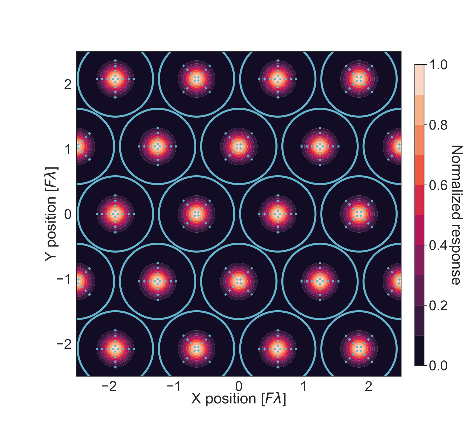
Plugging Eq. (44) into Eq. (43) yields a simple relationship between and aperture stop spillover efficiency
| (45) |
where is the F-number at the focal plane and . This assumption of Gaussian spillover efficiency does not necessarily hold when , as diffraction at the pixel edges will create substantial ringing in the far-field beam pattern. However, in an effort to remain agnostic to the specifics of the detector coupling architecture, we assume that Eqs. (43) and (45) remain valid for all values of in the calculations that follow.
While detector pixels can be arranged in a variety of ways, we must select a specific focal plane arrangement to find explicitly. In the calculations that follow, we assume hex-packed circular pixels, and we assume that pixel pitch is equal to pixel diameter . This assumption allows us to relate pixel packing density to pixel size as , where is the number of pixels per unit focal plane area. In practice, a small amount of dead space typically exists between pixels that does not scale with pixel size, and in this case, a more complex relationship between and is needed Padin 2010. However, these details are experiment specific and are therefore beyond the scope of the following discussions.
We note that the correlation calculation in Sec. 4 does not rely on most of the assumptions presented in this subsection. Specifically, only the detector beam’s assumed polarization properties are relevant to the HBT coefficient estimation. All the other assumptions related to the shape of the detector beam, the beam waist, and pixel packing are used only to calculate an explicit instrument sensitivity in Sec. 5 and Sec. 6.

4 Correlation calculation
Given the optical and detector models presented in Sec. 3, we now find the correlation patterns at the focal plane due to thermal radiation within the aperture and from the stop. A schematic of the radiation model for the central detector pixel is shown in Fig. 8.
4.1 Stop radiation
The stop is located in the far field of the detectors and is effectively a black, annular source with temperature . We therefore model the stop as a collection of infinitesimal, Gaussian-random, uncorrelated thermal emitters that generate Lambertian spherical wavelets, as shown in Fig. 8. These point sources represent atomic thermal motion within the stop’s absorbing material, and their wavelets superpose to form incoherent waves that the objective lens focuses onto the focal plane.
The above stop radiation treatment relies on two assumptions, which we justify here. First, while we consider the stop as a collection of uncorrelated thermal sources, it is known that blackbody radiators have non-zero correlation over the distance of a wavelength Mehta and Wolf 1964; Carter and Wolf 1975; Baltes et al. 1976; Steinle and Baltes 1977. However, as we will show in Sec. 4.2, Sec. 4.3, and Appendix B, this discrepancy leads to negligible errors for the calculations in this paper. Second, we assume for simplicity that all stop radiation reaches the detectors by propagating through all optics between the aperture plane and the focal plane, which impractically requires infinite optical throughput. That said, the cold box’s radiation environment has temperature , and the detectors sense that radiation when , regardless of the optical configuration. Therefore, our simplifying assumption of infinite optical throughput accurately accounts for stop-generated photons at each detector’s input.
4.2 Aperture radiation
Radiation incident on the sky side of the aperture (right side of Fig. 8) can be regarded as blackbody emission99 9 We assume that the incident radiation is largely unpolarized, or in terms of Stokes . This is a good approximation for millimeter and submillimeter telescopes. Consideration of polarized sources, which is outside the scope of this paper, can be found elsewhere Tervo et al. 2013. with an effective brightness temperature . Here, is defined such that is the mean occupation number of the blackbody radiation within the aperture. This mean occupation number can be written by adopting the definitions in Sec. 2.4 (Fig. 4 and Eqs. 37–39) and using , , as
| (46) |
where labels the aperture stop element. This blackbody radiation can be decomposed into plane-wave modes, and the FOV-filling nature of the sources (Sec. 3.1) ensures the above stated radiation property for all plane-wave modes whose propagation direction is within the FOV.1010 10 While plane-wave modes with propagation vector outside the FOV may have different radiation properties, they are irrelevant in our context of evaluating photon correlation among detectors.
We then consider a virtual, infinitely large sheet at that consists of Gaussian-random, infinitesimal, uncorrelated thermal emitters of temperature that generate Lambertian spherical wavelets. Radiation from these virtual emitters has equivalent statistical properties to the sky-side radiation in Fig. 8 so long as the distances from the sheet are significantly larger than the wavelength . To calculate this virtual sheet’s aperture truncation, we can simply remove elements outside of the aperture area . In Sec. 4.3 and Fig. 9, we compare aperture-truncated plane waves with this sheet of emitters and demonstrate their equivalence.
There is a small error that arises from the presented aperture emitter treatment. As noted above, the virtual sheet’s statistics become that of blackbody radiation at distances sufficiently larger than , and as noted in Sec. 4.1, non-zero correlations arise between emitters separated by . Thus, the emitter-sheet model deviates from that of aperture truncation in the region of and . Therefore when , aperture truncation produces additional non-trivial correlations that include polarization Chuss et al. 2008, but when , as is true for any reasonable telescope design, the correction can be safely neglected.
In summary, the VCZT coefficient can be calculated using the radiation field from a sheet of infinitesimal thermal emitters at with temperature at and at .
4.3 Intensity correlation patterns
Here we calculate spatial correlation patterns for the geometry in Fig. 5 while neglecting the polarization degree of freedom, similarly to Sec. 2.2. We then consider polarization in the next subsection. Consider the classical-wave electric field amplitude detected by detector at location . The detected partial amplitude due to an infinitesimal source area at the aperture plane can then be written as
| (47) |
Here, is the aperture illumination function for detector , and denotes the propagation direction of the incident plane wave focused by the objective lens onto detector , which can be related to the detector’s focal plane position via the objective’s focal length as
| (48) |
The illumination function is mapped from the detector’s angular-response function (Eq. (43)) via the telescope’s optics. We adopt the following normalization
| (49) |
which leads to
| (50) |
where the aperture stop spillover efficiency is defined in Eq. (45).
The non-polarized mutual intensity between detectors and can be written as a sum of contributions from the aperture radiation and stop radiation
| (51) |
The aperture-radiation component can then be written as
| (52) |
where , , , and , and where the second equality assumes that and that is approximately circularly symmetric. The VCZT coefficient (Eq. (10)) for the aperture radiation is
| (53) |
For our purpose of estimating the degree of coherence, a Gaussian illumination function is a good enough approximation:
| (54) |
In an extreme example of a flat illumination function (or ), Eq. (53) reduces to
| (55) |
where is the Bessel function of the first kind. This form is equivalent to the intensity diffraction pattern from a circular aperture, mirroring the well-known correspondence between diffraction and coherence formalisms (e.g., see Ref. Wolf 2007b). As discussed in Appendix C, Eq. (55) turns out to be a very good approximation for a general Gaussian illumination function when we assume the relation between the detector’s beam and pixel diameter discussed in Sec. 3. We thus use this handy approximation hereafter.
The stop-radiation component and can be calculated similarly to Eqs. (52) and (53) but instead using and integrating over :
| (56) |
and
| (57) |
As discussed in Appendix C, this term can also be approximated using a flat illumination and limiting the range of integration to . We then obtain the approximation
| (58) |
with
Figure 9 shows spatial HBT correlation patterns for both aperture and stop radiation calculated using their respective VCZT coefficients. As a demonstration, Fig. 9 also shows Monte-Carlo simulations where we directly calculate the (classical) intensity correlation coefficient by propagating fields to detectors and from complex Gaussian-random emitters on the stop and from complex Gaussian-random plane-wave modes incident on the aperture. We set the aperture diameter to , the stop’s outer diameter to , which simulates the case of , and the f-number to . We then simulate 3,000 realizations the aperture and stop fields. For radiation from the stop, we integrate Gaussian-random emitters over a grid with cell size .1111 11 The chosen grid spacing corresponds approximately to the coherence length of the simulated thermal radiation and therefore is small enough to represent the stop as a completely incoherent source. See Appendix B for more details. For radiation within the aperture, we simulate 2,500 total plane-wave modes (50 for each of and wave-number grids) distributed over the incident solid angle, which is enough to both resolve the aperture’s edges and Nyquist sample the integration grid. As expected, the Monte-Carlo simulation yields consistent results with the semi-analytic calculation of HBT coefficients in Eqs. (53) and (56).
Combining the aperture- and stop-radiation components, we obtain the VCZT coefficient for the assumed optical system
| (59) |
where is defined in Eq. (34) and satisfies
| (60) |
Equation (59) provides a general prescription to calculate the optical intensity correlation coefficient for bolometric detectors given a pixel spacing and an optical system parameterized by , , and . In addition, Eqs. (55) and (58) can be used as handy approximations to evaluate Eq. (59), such as for the sensitivity estimations in Sec. 5.
4.4 Polarized correlation patterns
Following the assumptions for telescope optics in Sec. 3.1 and detector parameters in Sec. 3.2, we show here that the polarized correlation pattern becomes the same as those derived in Sec. 2.3.
We consider detector pixels and and assume that each pixel has two detectors and with orthogonal polarization angles and following the beam patterns defined in Eqs. (23) and (24), respectively. As described in Sec. 2.3, each infinitesimal thermal source area on the aperture plane emits radiation with two independent Ludwig-3 polarizations and . This radiation couples to polarized plane-wave modes and that propagate along direction , and the telescope transforms these plane waves into spherical waves with polarization patterns and , as described in Eq. (41). In the reverse-time sense, the plane-wave modes radiating from detectors and correspond to plane-wave polarization vectors
| (61) |
respectively, when passing through the aperture. We note here that does not cross-couple to , and we assume that our ideal telescope generates no cross polarization.
Given the above assumptions, the polarization degree of freedom introduces a factor of and for the coupling between detector and the and emitters, respectively, with similar behavior for detector . The rest of the calculation proceeds exactly as in Sec. 2.3, following the results in Eqs. (26), (27), (28), and (29) that relate the unpolarized HBT coefficient to the Stokes coherence as
| (62) |
It is worth noting that the results derived here indicate zero correlation between two orthogonal detectors on different pixels and when . This finding contrasts the situation for planar blackbody radiators (or absorbers), where a non-zero correlation structure arises between radiation from one location and radiation from another Mehta and Wolf 1964. This difference comes from our assumption that the detector beam has an ideal Ludwig-3 polarization pattern with -plane symmetry. For emitters on a surface, modes project onto the the directions with a factor of and are therefore not -symmetric, hence introducing coherence along the two orthogonal directions.1212 12 One may regard this discrepancy as an artifact of the modal definition, as a fraction of the surface emitter’s modes projects to the direction. For the case of ideal Ludwig-3 detectors, all modes are distributed between the two orthogonal detectors, which results in -plane symmetry.
4.5 VCZT’s assumptions and applicability
The van Cittert-Zernike Theorem (VCZT) relies on a few assumptions, and thus its application has limitations (e.g., see Ref. Thompson et al. 2017 and references therein). We now comment on these assumptions and justify the applicability of the VCZT formalism to the intensity coherence calculation for millimeter and submillimeter telescopes.
First, the VCZT in its simplest form assumes scalar waves without a polarization degree of freedom and that the detectors are in the far-field of the source so that the Fraunhofer approximation can be used. That said, our -matrix based formalism accommodates general mode-to-mode coupling and therefore does not rely on these assumptions. Second, VCZT assumes completely incoherent sources, but our formalism assumes blackbody radiators, which exhibit a coherence length of . Appendix B shows that this one-wave coherence length can be ignored and therefore that our application of VCZT to blackbody sources is justified. Third, when considering amplitude coherence, we require to avoid the problem of decoherence. In contrast, decoherence does not occur for intensity coherence as noted in Sec. 2.1 and therefore no such bandwidth limit exists for calculations in this paper.
5 Impact of correlations on sensitivity
Using Eqs. (59), (17), and (62), we now investigate the impact of detector-to-detector correlations on instrument sensitivity, which is the primary goal of this paper. As shown in Fig. 9, detector outputs can correlate if their pixel pitch is , and these correlations will slow noise averaging during coaddition and therefore degrade array sensitivity.1313 13 Strictly speaking, a positive correlation between neighboring pixels can technically improve sensitivity when the angular diameter of interest approaches the pixel spacing projected on the sky (e.g., for Sunyaev Zel’dovich galaxy cluster surveys). In this section, we introduce a formalism for mapping speed, which measures the total sensitivity of the detector array, and we inspect the impact of HBT correlations on mapping speed vs. pixel size, which is a key metric used for focal plane design.1414 14 The code used to generate plots in this section can be found at https://github.com/chill90/HBT-Correlations.
5.1 Mapping speed
We assume that each detector in the imaging array has three noise components: photon shot noise, photon wave noise, and internal noise. The covariance between detection output ports and is
| (63) |
and the total variance of the detector array is
| (64) |
which effectively quantifies the instrument’s array-averaged sensitivity.
To both simplify and clarify the calculations that follow, we assume that all detectors in the array have the same noise properties. Internal detector noise and photon shot noise cannot correlate between outputs, which allows the covariance to be written as
| (65) |
where is the HBT coefficient and where , , and are the variances of the shot, wave, and internal noise components, respectively, for every detector in the array. While array uniformity is not in general true for real experiments, it is common practice to use the median noise expectation when forecasting instrument performance, making a uniform treatment useful for instrument designers. Additionally, the details of detector-to-detector variation are experiment-dependent and are therefore beyond the scope of this paper.
Given the simplification in Eq. (65) and noting that , the total variance of the detector array can be written as
| (66) |
The first term represents uncorrelated array noise while the second term quantifies noise augmentation due to HBT correlations. Let us further define an array-averaged correlation coefficient across the detector array as
| (67) |
which allows us to write the array sensitivity more compactly as
| (68) |
In this form, the impact of intensity correlations on the detector array noise is reduced to calculating the array-averaged HBT coefficient . In the limit of , and the array-averaged wave noise is not at all suppressed by detector coaddition. This fact drives the use of interferometers at low frequencies where , where , and where correlation lengths are long for astronomical sources. In the other limit of , wave noise averages in the familiar way for uncorrelated measurements . It is worth emphasizing that the augmentation of by not only depends on the HBT coefficient but also on the relative contribution of wave noise to that of the other noise terms. As shown in Eq. (36), while , and therefore becomes more important at lower frequencies and higher brightness temperatures.
Internal detector noise depends on many factors, including the detector’s architecture, thermal noise properties, amplifier noise properties, linearity, and dynamic range, among other things. To remain agnostic to these experiment-specific characteristics, we set hereafter, noting that modern mm-wave observatories aim to be photon-noise dominated.1515 15 For the ubiquitous transition-edge sensor (TES) bolometric detectors Richards 1994; Lee et al. 1997, internal thermal noise is proportional to the detector’s saturation power , where is the detected optical power and is the detector bias power Mather 1982. Therefore, scaling and together during experiment design and optimization, while not an exact metric, is well motivated.
Finally, we quantify the experiment’s signal-to-noise using its mapping speed, which is defined as the square ratio of the input signal to the array-averaged noise
| (69) |
Here, is the optical efficiency of the entire system, which is a product of the detector’s quantum efficiency (Eq. (31)), the aperture spillover efficiency (Eq. (45)), and all the other transmission efficiencies, including those of the telescope’s optical elements and the atmosphere. Mapping speed is a powerful measure of an experiment’s efficacy, as it is and is therefore analogous to detector yield and observation efficiency.
5.2 Pixel size optimization
Using the optics and detector assumptions in Sec. 3 and the VCZT and HBT coefficients in Eqs. (59), (17), and (62), we now calculate mapping speed vs. pixel size. Provided a fixed FOV, or equivalently a fixed focal plane size, decreasing pixel diameter increases the number of detectors as but decreases aperture spillover efficiency as . These competing effects combine to form a peak in mapping speed vs. pixel size, which reveals the optimal packing density.
An example “classic” mapping speed vs. pixel size curve Griffin et al. 2002; Arnold 2010; Suzuki 2013; Datta et al. 2014; Cukierman et al. 2018—one for which —of a model 90 GHz instrument with a 4 K stop is shown in Fig. 10. Historically, ground-based CMB experiments have observed at 95, 150, and 220 GHz with Arnold 2010; Henning et al. 2012; Suzuki 2013; Thornton et al. 2016; Simon et al. 2016; Simon et al. 2018; Posada et al. 2018; Hui et al. 2016; Schillaci et al. 2020; Dahal et al. 2020 where the HBT correlation coefficient is small. However, as new readout architectures become available Dobbs et al. 2012; Dober et al. 2017 and as CMB experiments push to lower frequencies for improved synchrotron characterization Li et al. 2018; Xu et al. 2020; Zhang et al. 2020, focal planes with are becoming increasingly practical. Therefore, the impact of HBT correlations on mapping speed is of interest to upcoming mm-wave experiments, such as CMB-S4 Abitbol et al. 2017. In this section, we calculate HBT-modified mapping speed vs. pixel size curves for our model telescope at several observation frequencies, and we discuss the results.
We assume that our telescope is ground-based with cryogenically cooled optics, infrared filters, and sub-Kelvin detectors. As shown in Eq. (46), radiation at the aperture plane can be summed over all sky-side sources and represented by a single effective brightness temperature . To simplify and generalize the following analysis, we assume only three sources viewed through the aperture: the CMB with , the atmosphere with , and telescope optics with . The telescope’s effective temperature can vary considerably depending on the specifics of the mirrors, ground shield, cryostat window, and anti-reflection coatings, but as an example, we assert a default configuration where K. We also assert the stop’s physical temperature to be K and that each detector’s quantum efficiency is . To model power due to atmospheric emission, we assume that the telescope observes from the the Chajnantor Plateau in the Atacama Desert of Chile, and we use the AM model Paine 2019 to generate the atmosphere’s effective brightness temperature and transmittance at 1 mm precipitable water vapor (PWV) and 50 deg elevation above the horizon.
Given this telescope + sky model, we consider four top-hat observation bands centered at (35, 95, 150, 220) GHz with bandwidths of (17, 33, 39, 44) GHz. The chosen bands, along with , , and , are shown in Fig. 11. The channels are chosen to fit within atmospheric windows and are similar to those of existing Atacama instruments. Additionally, Fig. 11 shows the bunching fraction for each frequency band vs. sky temperature at , where . As discussed in Sec. 5.1, while lower-frequency modes tend to have larger occupation numbers, the sky is brighter at higher frequencies, and therefore correlations substantially impact sensitivity in all four bands.
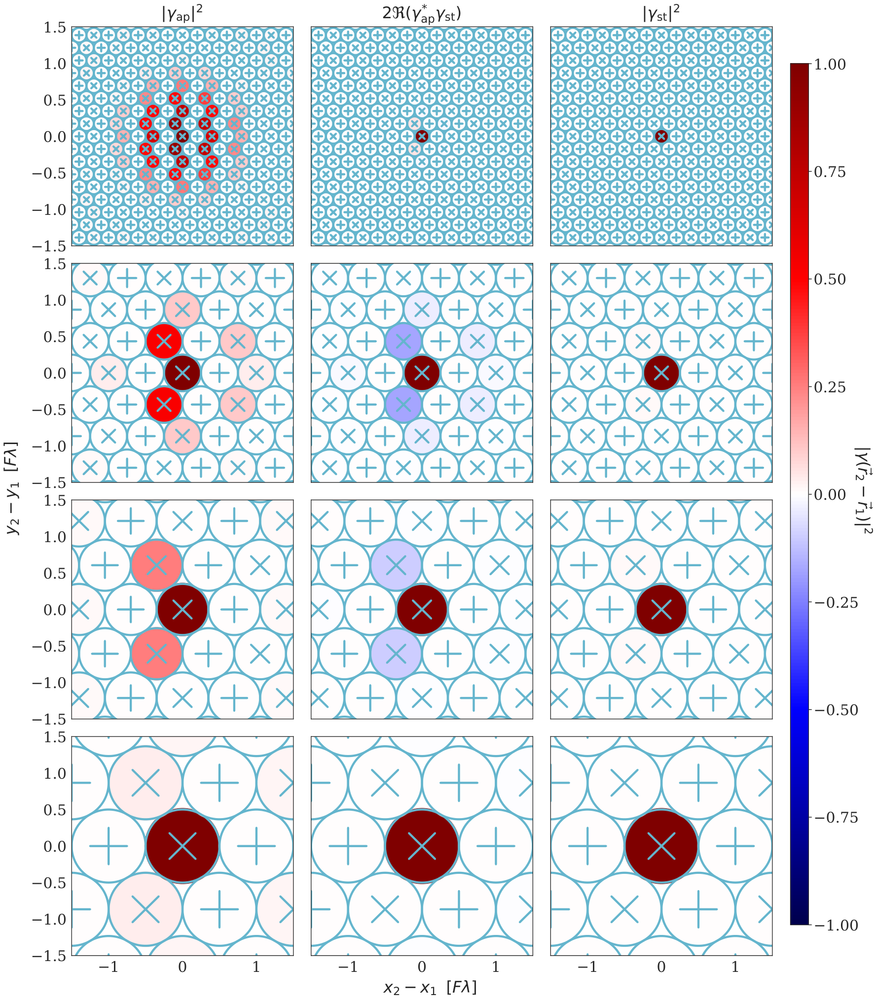
Fig. 12 shows an example of four pixel pitch scenarios given the hex packing described in Sec. 3.2, and the contour shows the Stokes HBT coefficient due to both aperture and stop radiation. As expected, the degree of correlation is a two-dimensional version of the VCZT curves in Fig. 9. The effect of pushing is for the detected modes (the pixel apertures) to oversample the input modes (the contour), giving rise to correlated noise between nearby detectors.
When calculating Stokes mapping speed, we sum the HBT coefficients in Fig. 12 over a 4 radius to find
| (70) |
noting that because each pixel has two orthogonal polarimeters, vanishes for half of all output pairs. The impact of HBT correlations becomes roughly twice when considering mapping speed for measurements of intensity or Stokes . We then assume that this sum applies to all detectors on the focal plane such that . This treatment ignores the fact that edge pixels have fewer neighbors than internal ones, which is a reasonable approximation for focal planes of large area. For small or moderately-sized detector arrays, the fraction of edge pixels may become important, but such details are experiment-dependent and are therefore beyond the scope of this paper. Fig. 13 shows HBT-impacted mapping speed vs. pixel size curves for each observation band, normalized to the peak of the “classic” curve for which . Three additional mapping speed curves with in-aperture loading from only the CMB, only the atmosphere, and only the telescope are also plotted to demonstrate the dependence of HBT correlations on various source temperatures.
There are several features in Fig. 13 that are worth noting explicitly. Firstly, the impact of HBT correlations depends on source temperature and is most pronounced in the presence of a brightly illuminated aperture. This effect is most clearly seen when contrasting the CMB and atmosphere, especially at 220 GHz where the CMB’s photon occupation number is falling while that of the atmosphere is rising. Secondly, while HBT correlations impact curve shape most prominently at low frequencies, the atmosphere is brighter at higher frequencies, inducing a similar HBT suppression across all bands. Thirdly, the mapping speed peak is located at a slightly larger than that of the classic curves at 35 and 95 GHz but resides at a similar location to that of the classic curves at 150 and 220 GHz. This effect arises because the stop is significantly fainter than the sky at 150 and 220 GHz, and therefore as falls below , decreases less rapidly than . Lastly, the impact of correlations on mapping speed starts to become most important when , but there also percent-level impacts at larger spacings, which correspond to local maxima in the aperture/stop VCZT patterns, as shown in Fig. 9. This effect gets smoothed out when averaging the HBT coefficients across each channel’s finite bandwidth. Regardless of the input assumptions in this section, the mapping-speed gain by undersized pixels when is suppressed compared to the classic case, especially for ground-based telescopes.
6 Implications for experiment design
As shown in Fig. 13, HBT correlations both modify the optimal pixel packing density and suppress the achievable mapping speed with respect to the “classic” calculation. However, the degree of modification depends on a plethora instrument details, including internal detector noise, observation site and conditions, stop temperature, detector efficiency, telescope optical throughput, and extraneous noise sources, such as electromagnetic interference, vibrational pickup, and detector nonidealities. A more comprehensive handling of correlations within a more general experiment is available via the BoloCalc sensitivity calculator Hill et al. 2018, but in this section, we sweep a few parameters in our model telescope to serve as a quick reference for focal plane designers. The results of these calculations are shown in Fig. 14.
The first column of Fig. 14 shows mapping speed vs. pixel size for various stop temperatures K. As stop temperature decreases, so does photon loading due to stop spillover, which in turn favors smaller pixels. A colder stop also suppresses the relative contribution of , especially at higher frequencies, modulating the slope of the mapping speed curve below . The second column of Fig. 14 shows mapping speed vs. pixel size for various telescope temperatures K. As telescope temperature increases, so too does the photon load within the aperture, which in turn favors smaller pixels. In addition, brighter aperture radiation increases and hence also increases the HBT suppression. The third column of Fig. 14 shows mapping speed vs. pixel size in the presence of a constant internal detector noise at , where . As increases with respect to , larger pixel sizes are favored to improve signal strength via an increased . Simultaneously, the impact of HBT correlations is reduced due to a smaller relative contribution of and due to an optimum where is small.
These few examples only graze the rich topic of focal plane optimization, and we leave a more comprehensive discussion of experiment-specific applications to other publications. Nonetheless, regardless of the context, HBT correlations should be considered when designing dense focal planes, especially for ground experiments where the sky and telescope brightness temperatures are substantially larger than that of the CMB.
7 Conclusion
We have presented a theoretical formalism for photon noise correlations by extending the quantum optical circuit-based model in Zmuidzinas Zmuidzinas 2003 to a free-space classical model using the optical equivalence theorem of Glauber and Sudarshan Sudarshan 1963. We have used this formalism to estimate the Hanbury Brown-Twiss (HBT) coefficient Brown et al. 1952; Brown and Twiss 1954; Brown and Twiss 1956 in a simplified telescope optical system, and we have shown that these simulations match the expectation of the van Cittert-Zernike theorem (VCZT) van Cittert 1934; Zernike 1938. This equivalence allows the HBT coefficient to be calculated with only a knowledge of the radiation intensity profile at the aperture plane.
We then uniformly illuminated our model telescope with blackbody sources representative of radiation from the CMB, atmosphere, and telescope, and we have calculated the impact of HBT correlations on experiment mapping speed vs. pixel size within observation bands centered at 35, 95, 150, and 220 GHz. Acknowledging that sensitivity calculations have many inputs and assumptions, we have further discussed three useful variations to the simplified instrument—stop temperature, telescope temperature, and internal detector noise—and showed how each parameter modulates the HBT-modified mapping speed curves. This work builds on an initial discussion by Padin Padin 2010 and formalizes the calculation of photon noise correlations between detector pixels in millimeter and sub-millimeter telescopes for astronomy. The presented formalism and results are useful to GHz focal plane designers, especially as emerging readout technologies enable the deployment of dense detector arrays.
Acknowledgement
Work at LBNL is supported by the U.S. Department of Energy, Office of Science, Office of High Energy Physics under contract No. DE-AC0205CH11231. We acknowledge the support by JSPS Grant Number JP19K21873. We thank our Simons Array and Simons Observatory colleagues for fruitful discussions on CMB telescope designs, and we thank Masahito Ueda for teaching us some of the basics of quantum statistical mechanics.
Appendix A Thermal photon density matrix
The statistical state, or the mixed state, of photons can be described using density matrix . We consider a single-mode photon state, where the state is single-moded in both spatial and frequency domains as well as in polarization state. Using creation and annihilation operators and , respectively, the density matrix can be written as that of a Bose-Einstein distribution
| (71) |
with
| (72) |
Here, is the Fock state and is a mean occupation number. We consider a detection process whose integration time (the inverse of sampling rate) is significantly longer than the coherence time , where is the detection bandwidth. This is usually the case for a CMB instrument, where and . In this situation where , the mean occupation number can be written as
| (73) |
We can now rewrite the density matrix in terms of Glauber’s coherent state . The coherent state is written as
| (74) |
and satisfies
| (75) |
The density matrix can be rewritten in the Glauber-Sudarshan representation Sudarshan 1963; Glauber 1963a as
| (76) |
with
| (77) |
where the integral is over the entire complex plane. Here, the complex amplitude follows a Gaussian distribution , in agreement with the expectation in the classical limit. The photon counting of a coherent state follows a Poisson distribution as
| (78) |
Eqs. (76) and (78) immediately lead to a special case of Mandel’s formula Mandel 1958; Mandel 1959
| (79) |
Appendix B Partial Coherence of Sources
In this paper, we assume complete incoherence between two source elements that are physically apart from one another. However, it is known that blackbody sources have finite correlation at the length scale of a wavelength Mehta and Wolf 1964; Carter and Wolf 1975; Baltes et al. 1976; Steinle and Baltes 1977. The effect of source coherence on the applicability of VCZT for quasihomogeneous sources, whose spatial intensity variations are slow compared to its coherence length, are extensively discussed in literature Wolf and Carter 1975; Wolf and Carter 1976; Carter and Wolf 1977; Friberg 1982. Thus, it is worthwhile to clarify the assumptions in this paper regarding source coherence. In the end, we find that the assumption of completely incoherent sources is a good approximation for telescope systems relevant to our discussion. We first consider source coherence for the simple case presented in Sec. 2.2, which is readily comparable to examples in the literature. We then discuss source coherence in the general formalism of Sec. 2.1.
Equation (20) in combination with (10) constitutes VCZT of a completely incoherent source for the simple geometry in Fig. 2. For sources with partial coherence (e.g., see Ref. Thompson et al. 2017), the first-order coherence is
| (80) |
with
| (81) |
where and are the positions of detectors and , respectively, and where is the coherence of the field between locations and on the source surface . Here, we assume that the source’s coherence is statistically isotropic and thus that the source coherence function can be written as . Complete incoherence of the source corresponds to the limit of and we immediately find that Eq. (80) reduces to Eq. (20) in such a limit.
We define a coherence length such that for . For blackbody radiators, since we assume detectors with a limited detection band.1616 16 See, e.g., Ref. Mehta and Wolf 1964 for consideration without a band limit. Focusing on cases where is significantly smaller than the source size, Eq. (80) can be approximated as
| (82) | ||||
| (83) |
with
| (84) |
where is the angle between and the source plane’s normal vector. The expression in Eq. (83) becomes equivalent to Eq. (20) when can be regarded as a constant function of .
To evaluate , we consider a blackbody surface source that may not be centered at , and we assume that the solid angle of the source is small compared to . We consider two regions of the parameter space depending on the source’s position. Region 1 is when . In this case,
| (85) |
and thus and Eq. (83) becomes equivalent to Eq. (20). Region 2 is when . In this case, is approximately constant across the source , and thus where is the mean of for the source . The factor maps to the radiance reduction due to source coherence, which shows up in and as well. Thus, the normalized amplitude coherence remains identical to the case of a completely incoherent source, which is consistent with results presented in the literature Carter and Wolf 1977. When the source comprises Lambertian blackbody emitters, the radiance satisfies by construction.
In summary, for a source with the geometry assumed in Sec. 2.2, partial coherence between spatially independent blackbody radiators can be neglected and Eq. (20) is a good approximation.
We now look to Sec. 2.1, which considers a more general, VCZT-free formalism. For quasihomogeneous sources with partial coherence, in contrast to completely incoherent sources, the Kronecker delta in Eq. (3) is replaced by a source coherence function . The mutual intensity is then expressed as
| (86) |
where the index denotes each quasihomogeneous source with a temperature , and is the coherence function of the source. Equation (86) is the generalized version of Eq. (80). Similarly to Eq. (83), we can decompose Eq. (86) as
| (87) |
with
| (88) |
where is a collection of modes close enough to mode such that is non-zero. The expressions for normalized coherence, both and , become identical to the case with completely incoherent sources if is constant across .1717 17 Strictly speaking, reducing modifies the normalized coherence from the case with complete incoherence. However, these changes in lead to changes in apparent brightness temperature, which can be absorbed into , and therefore the formal equivalence for the normalized coherence still holds. Whether can be regarded as constant should be evaluated on a case-by-case basis.
For the cases discussed in this paper, we can regard as constant given the following arguments. For aperture radiation, and correspond to modes emitted by infinitesimal sources at and , respectively. Using Eqs. (47) and (48), can be written as
| (89) |
with the integrated region being
Since , the aperture illumination function varies minimally within the integrated range and thus . The source coherence function is isotropic and thus depends only on as , leading to
| (90) |
with
Thus, is constant as a function of and source coherence can therefore be ignored.
For stop radiation, the physical geometry may be more complicated than for the aperture radiation, and therefore may sometimes vary across the source. However, because typically varies slowly compared to , we can divide the source into sections that are significantly larger than and in which is effectively constant. Given this setup, we can ignore source coherence by regarding each of these sections as independent sources indexed by in Eq. (86).
In summary, for the model optical system presented in Sec. 3, the assumption of completely incoherent sources is a good approximation for the context of this paper.
Appendix C Goodness of Flat-Illumination Approximation
C.1 Aperture Radiation
In this section, we show that Eq. (55) is a good approximation of Eq. (52) even for a general Gaussian illumination function . The key assumption is that the beam can be approximated by Eqs. (43) and (44) and that the pixel spacing satisfies
| (91) |
As described in Sec. 4.3 and Eq. (54), we approximate the illumination function as
| (92) |
and as described in Eq. (43), the circumference of the aperture corresponds to an angle of . It thus follows that
| (93) |
assuming a linear mapping from detector-beam angle to aperture position .
C.2 Stop Radiation
As Fig. 12 suggests, stop radiation contributes only minorly to the total correlation among pixels. To demonstrate this contribution explicitly, Fig. 16 shows for various of the Gaussian illumination in Eq. (92). When , the VCZT coherence asymptotes to a Dirac delta function and thus contributes negligibly to the intensity correlation. In the other limit of , asymptotes to zero and the stop becomes irrelevant.
The contribution of stop radiation may become non-negligible, though still small, when is in neither of these limits, or when . In this parameter region, an approximation can be obtained by calculating the coherence of a flat-illuminated annulus with width
| (94) |
where
The dashed lines in Fig. 16 show this approximation for a few relevant examples.
References
- Fano (1961) U. Fano, American Journal of Physics 29, 539 (1961).
- Glauber (1963a) R. J. Glauber, Physical Review 131, 2766 (1963a).
- Glauber (1963b) R. J. Glauber, Physical Review Letters 10, 84 (1963b).
- Mandel and Wolf (1963) L. Mandel and E. Wolf, Physical Review Letters 10, 276 (1963).
- Carter and Wolf (1975) W. H. Carter and E. Wolf, JOSA 65, 1067 (1975).
- Carter and Wolf (1977) W. H. Carter and E. Wolf, JOSA 67, 785 (1977).
- Brown et al. (1952) R. H. Brown, R. C. Jennison, and M. K. D. Gupta, Nature 170, 1061 (1952).
- Brown and Twiss (1954) R. H. Brown and R. Q. Twiss, The London, Edinburgh, and Dublin Philosophical Magazine and Journal of Science 45, 663 (1954).
- Brown and Twiss (1956) R. H. Brown and R. Q. Twiss, Nature 177, 27 (1956).
- Padin (2010) S. Padin, Applied Optics 49, 479 (2010).
- Zmuidzinas (2003) J. Zmuidzinas, Applied Optics 42, 4989 (2003).
- van Cittert (1934) P. H. van Cittert, Physica 1, 201 (1934).
- Zernike (1938) F. Zernike, Physica 5, 785 (1938).
- Hill et al. (2018) C. A. Hill et al., Proc. SPIE 10708, 1070842 (2018), eq. (4) has a typo and a corrected version is available on arXiv (arXiv:1806.04316v2).
- Sudarshan (1963) E. C. G. Sudarshan, Physical Review Letters 10, 277 (1963).
- Wolf (2007a) E. Wolf, Introduction to the Theory of Coherence and Polarization of Light (Cambridge University Press, 2007) p. 130.
- Ludwig (1973) A. Ludwig, IEEE Transactions on Antennas and Propagation 21, 116 (1973).
- Kildal (2000) P.-S. Kildal, Foundations of Antennas A Unified Approach (Studentlitteratur AB, 2000).
- Stutzman and Thiele (1997) W. L. Stutzman and G. A. Thiele, Antenna Theory and Design (Wiley, New York, 1997).
- Zeng et al. (2010) L. Zeng, C. L. Bennett, D. T. Chuss, and E. J. Wollack, IEEE Transactions on Antennas and Propagation 58, 1383 (2010).
- Kusaka et al. (2014) A. Kusaka, E. J. Wollack, and T. R. Stevenson, J. Opt. Soc. Am. A 31, 1557 (2014).
- Baltes et al. (1976) H. P. Baltes, B. Steinle, and G. Antes, Optics Communications 18, 242 (1976).
- Wolf and Carter (1975) E. Wolf and W. H. Carter, Optics Communications 13, 205 (1975).
- Wolf and Carter (1976) E. Wolf and W. H. Carter, Optics Communications 16, 297 (1976).
- Wolf (1978) E. Wolf, JOSA 68, 6 (1978).
- Agarwal et al. (2004) G. S. Agarwal, G. Gbur, and E. Wolf, Optics Letters 29, 459 (2004).
- Mizugutch et al. (1976) Y. Mizugutch, M. Akagawa, and H. Yokoi, IEEE International Symposium on Antennas and Propagation Digest , 2 (1976).
- Dragone (1978) C. Dragone, Bell System Technical Journal 57, 2663 (1978).
- Tran et al. (2008) H. Tran, A. Lee, S. Hanany, M. Milligan, and T. Renbarger, Applied Optics 47, 103 (2008).
- Mehta and Wolf (1964) C. L. Mehta and E. Wolf, Physical Review 134, A1143 (1964).
- Steinle and Baltes (1977) B. Steinle and H. P. Baltes, JOSA 67, 241 (1977).
- Tervo et al. (2013) J. Tervo, T. Setälä, J. Turunen, and A. T. Friberg, Optics Letters 38, 2301 (2013).
- Chuss et al. (2008) D. T. Chuss, E. J. Wollack, S. H. Moseley, S. Withington, and G. Saklatvala, Publications of the Astronomical Society of the Pacific 120, 430 (2008).
- Wolf (2007b) E. Wolf, Introduction to the Theory of Coherence and Polarization of Light (Cambridge University Press, 2007).
- Thompson et al. (2017) A. R. Thompson, J. M. Moran, and J. Swenson, George W., in Interferometry and Synthesis in Radio Astronomy, 3rd Edition (Springer, 2017) Chap. 15, pp. 767–786.
- Richards (1994) P. L. Richards, Journal of Applied Physics 76, 1 (1994).
- Lee et al. (1997) A. T. Lee, J. M. Gildemeister, S.-F. Lee, and P. L. Richards, IEEE Transactions on Applied Superconductivity 7, 2378 (1997).
- Mather (1982) J. C. Mather, Applied Optics 21, 1125 (1982).
- Griffin et al. (2002) M. J. Griffin, J. J. Bock, and W. K. Gear, Applied Optics 41, 6543 (2002).
- Arnold (2010) K. S. Arnold, Ph.D. Thesis (2010).
- Suzuki (2013) A. Suzuki, Ph.D. Thesis (2013).
- Datta et al. (2014) R. Datta et al., Journal of Low Temperature Physics 176, 670 (2014).
- Cukierman et al. (2018) A. Cukierman, A. T. Lee, C. Raum, A. Suzuki, and B. Westbrook, Applied Physics Letters 112, 132601 (2018).
- Henning et al. (2012) J. W. Henning et al., Proc. SPIE 8452, 84523A (2012).
- Thornton et al. (2016) R. J. Thornton et al., The Astrophysical Journal Supplement Series 227, 21 (2016).
- Simon et al. (2016) S. M. Simon et al., Proc. SPIE 9914, 991416 (2016).
- Simon et al. (2018) S. M. Simon et al., Journal of Low Temperature Physics 193, 1041 (2018).
- Posada et al. (2018) C. M. Posada et al., Journal of Low Temperature Physics 193, 703 (2018).
- Hui et al. (2016) H. Hui et al., Proc. SPIE 9914, 99140T (2016).
- Schillaci et al. (2020) A. Schillaci et al., Journal of Low Temperature Physics 199, 976 (2020).
- Dahal et al. (2020) S. Dahal et al., Journal of Low Temperature Physics 199, 289 (2020).
- Dobbs et al. (2012) M. A. Dobbs, M. Lueker, et al., Review of Scientific Instruments 83, 73113 (2012).
- Dober et al. (2017) B. Dober et al., Applied Physics Letters 111, 243510 (2017).
- Li et al. (2018) Y. Li et al., Proc. SPIE 10708, 8 (2018).
- Xu et al. (2020) Z. Xu et al., The Astrophysical Journal 891, 134 (2020).
- Zhang et al. (2020) C. Zhang et al., Journal of Low Temperature Physics 199, 968 (2020).
- Abitbol et al. (2017) M. H. Abitbol, Z. Ahmed, D. Barron, et al., arXiv:1706.02464 [astro-ph] (2017).
- Paine (2019) S. Paine, “The am atmospheric model,” Zenodo (2019).
- Mandel (1958) L. Mandel, Proceedings of the Physical Society 72, 1037 (1958).
- Mandel (1959) L. Mandel, Proceedings of the Physical Society 74, 233 (1959).
- Friberg (1982) A. T. Friberg, Optical Engineering 21, 212362 (1982).