Robust Point Cloud Processing through Positional Embedding

An obvious strategy to obtain a permutation invariant lossless feature is to encode points with the impulse function:

$$\phi(t)=\sum_{i=1}^{N}h(x_{i},t)=\sum_{i=1}^{N}\delta(t-x_{i})\>,$$

(3)

where $\delta(\cdot)$ is the impulse function and $t\>{\in}\>(0,1)$. A drawback is that $\phi(t)$ becomes an infinite bandwidth signal, which means we need infinite feature dimensions in discrete space to represent it (observe that this is equivalent to doing one-hot encoding in a continuous space). Another drawback is that when there is noise in the points, the embedding obtained by the impulse function will have a large difference from the embedding of the clean point cloud. Additionally, the error between the clean point embedding and the noisy point embedding is not proportional to the noise intensity. Nonetheless, a common approximation to the impulse function is $\mbox{sinc}(x)\>{=}\>\frac{\sin(\pi x)}{\pi x}$, which is band-limited and easy to discretize. The feature can be represented as:

$$\phi(t)=\sum_{i=1}^{N}h(x_{i},t)=\sum_{i=1}^{N}\mbox{sinc}(K(t-x_{i}))\>,$$

(4)

where $K$ is a hyper-parameter that controls the bandwidth. Fig. 3 provides a visual example. Note that shifting a signal does not affect its spectrum, and the Fourier transform is a linear operation. Therefore, the bandwidth of $\phi(t)$ is $K$, and it can be represented as $K$ equally spaced, weighted sinc functions as,

$$\phi(t)=\sum_{k=1}^{K}\gamma_{k}\mbox{sinc}\left(K\left(t-u_{k}\right)\right)\>,$$

(5)

where $u_{k}$ are equally spaced (Nyquist Shannon sampling theorem). This can equivalently be represented in the Fourier domain as,

$$\phi(t)=\sum_{b=0}^{B-1}\gamma_{b}\mbox{cos}\left(2\pi bt\right)+\gamma_{b+B}\mbox{sin}\left(2\pi bt\right)\>,$$

(6)

where $B\>{=}\>\frac{K}{2}$, and $\gamma$s are coefficients.

For high-dimensional cases, like 3D for point clouds, all the axes need to be sampled and encoded, and then the embeddings are multiplied together to get a high-dimensional embedding. The drawback of sinc encoding is the huge number of bases required so that the encoding dimension is growing as a power to the input dimension. However, one huge advantage of sinusoids is that, although it seems no difference using sinc or sinusoids basis in 1D, in high dimensional cases sinusoids can provide a better encoding with much fewer feature dimensions by trigonometric identities. Theoretically, the number of terms of sinc or sinusoids basis in high dimension is the same. The distribution of these sinusoids is no longer uniform and tends towards a Gaussian whose variance is proportional to the bandwidth $B$. If one attempts to subsample from those huge numbers of basis, this non-uniform distribution offers a principled strategy for frequency selection. This gives some intuition on why random Fourier features (RFF) Tancik et al. 2020 are such an attractive embedding for higher dimensional cases. We explain the high-dimensional case in the appendix and refer the reader to Zheng et al. 2022 where this dilemma is discussed at length.

According to Zheng et al. 2021, a good embedding should also be smooth (i.e., distance preserving), which means closer point clouds in the input space have more similar features. The feature is also important for the robustness of the model. When the input point cloud has noise or outliers, a smooth per-point encoder can generate a similar embedding to the clean one. In the ideal case, feature distance should be proportional to the distance between input point clouds, which is

	$\displaystyle\mathrm{D}_{f}(\mathbf{y}_{1},\mathbf{y}_{2})$	$\displaystyle{\displaystyle=}\>\|\phi(\{x_{1,i}\}_{i=1}^{N},t){-}\phi(\{x_{2,i}\}_{i=1}^{N},t)\|^{2}_{2}$		(7)
		$\displaystyle{\displaystyle\propto}\>\sum_{i=1}^{N}\|x_{1,i}{-}x_{2,i}\|_{2}^{2}\>,$

where $\mathrm{D}_{f}$ is distance between features, $\{x_{1,i}\}_{i=1}^{N}$, $\{x_{2,i}\}_{i=1}^{N}$ are two point clouds and $\phi_{1}$, $\phi_{2}$ are their features.

When the PPE is not band-limited, such as the impulse function, this will not hold since no matter how far the point moves, the changes in the feature are the same. When the PPE is band-limited as we discussed in Section 3.1, based on the theory in Zheng et al. 2021, for each point, the encoding distance is proportional to the input distance, which means

$$\mathrm{D}_{e}(\mathbf{e}_{1},\mathbf{e}_{2})=\|\phi(x_{1},t){-}\phi_{2}(x_{2},t)\|^{2}_{2}\propto\|x_{1}{-}x_{2}\|_{2}^{2}\>,$$

(8)

where $\mathrm{D}_{e}$ means distance between encodings, $x_{1}$, $x_{2}$ are two point clouds and $\mathbf{e}_{1}$, $\mathbf{e}_{2}$ are their features. Although it is not necessarily equivalent, it strongly implies Eq. 7 will hold since features are just summation of encodings. In addition, a critical advantage of using our band-limited encoders is that one can easily tune the bandwidth of the representation by varying the variance of the frequency distribution. Zheng et al. 2021 shows that by varying the bandwidth, the distance preservation (or the feature similarity) between nearby point encodings can be controlled. This is a vital property that can be exploited when dealing with OOD data.

In the original PointNet architecture, the encoder is an MLP and the entire network is trained end-to-end. The deep ReLU point embedding for PointNet can be defined as

$$\mathcal{H}_{\ell}(\mathbf{x})=\mbox{ReLU}[\mathbf{W}_{\ell}\circ\mathcal{H}_{\ell-1}(\mathbf{x})+\mathbf{b}_{\ell-1}]\>,$$

(9)

where $\mathcal{H}_{0}(\mathbf{x})\>{=}\>\mathbf{x}$. The PPE in PCT can be defined as

	$\displaystyle\mathbf{F}_{1}$	$\displaystyle=\mbox{AT}^{1}(\mathbf{F}_{e})\>,$
	$\displaystyle\mathbf{F}_{i}$	$\displaystyle=\mbox{AT}^{i}(\mathbf{F}_{i-1})\>,\>i=2,3,4$
	$\displaystyle\mathbf{F}_{o}$	$\displaystyle=\mbox{concat}(\mathbf{F}_{1},\mathbf{F}_{2},\mathbf{F}_{3},\mathbf{F}_{4})\>,$

where $\mbox{AT}^{i}$ is the $i$-th attention layer, $\mathbf{F}_{e}$ is the input embedding through some MLPs and sampling and grouping layer, and $\mathbf{F}_{o}$ is the final embedding. The deep ReLU network and attention layers map low-dimensional encodings to a high-dimensional space. This mapping is band-limited and preserves distance information when randomly initialized. However, after training end-to-end with data, its ability to preserve distance entirely depends on the training data. There is no clear geometry information in the learned features, therefore, when OOD noise is added to the data, it is unpredictable how the features will change in the feature space and whether it will pass the decision boundary of the learned classifier or not.

Moreover, even though random initialized MLPs can be viewed as a non-trained per-point encoder, it is unclear how the initialization affects the behavior of the embeddings. On the contrary, PE has a well-established theory—by tuning the hyper-parameters (usually called “scale” in PE), we can theoretically know the bandwidth and smoothness changes and predict the performance of the embedding. The sinusoids encoder we discussed in Section 3.1 turns into PE—RFF, which is defined as

$$\mathcal{G}(\mathbf{x})=\begin{bmatrix}\cos(\mathbf{W}\mathbf{x})\\ \sin(\mathbf{W}\mathbf{x})\end{bmatrix}\>.$$

(10)

The distance preservation property of these three encoders is shown in Fig. 4. For the ReLU network, the distance is kept linearly in the point space, while for RFF, this property can be tuned by tuning the scale (standard deviation of random weight matrix). Even if we change the standard deviation of the ReLU network, i.e., multiply the weights with a specific scale, we will get an output that is also multiplied by that specific scale, instead of changing the shape of the distance preservation curve. Note that for RFF, when the scale is large, such as $\sigma{=}8$ (shown in Fig. 4), only local distance is preserved, which means only local information is concerned. This property makes the RFF encoder robust to noise and outliers.

As mentioned before, the architecture of PointNet and PCT can be divided into three parts, i.e., a PPE (ReLU-MLPs), a pooling function (max pooling), and a downstream network (fully connected networks, FCNs). Here, we introduce our settings for these three components separately.

We followed the standard training protocol in Sun et al. 2022 and trained all models on clean ModelNet40 Wu et al. 2015 data with $1024$ points and $300$ epochs. We did not use any data augmentation strategy except random scaling and translation as proposed in DGCNN Wang et al. 2019—which is usually considered as “unaugmented”. We show the classification results on clean data in the first columns of Table 2. We observed that end-to-end trained methods achieve good performance and PointNet++ has the lowest error rate. Both randomly initialized PE-AT and PE achieve comparable but slightly worse results compared to learned PointNet indicating the ability of PE-based methods in replacing learned PPEs.

To compare the robustness of different PPEs and pooling functions, we trained the model (the entire model or the classifier alone if PPEs do not need to train) on clean data and tested these trained models on test data under six different types of noise and outlier corruptions. We selected five noise/outlier types from ModelNet40-C Sun et al. 2022 dataset: uniform noise, Gaussian noise, impulse noise, upsampling outliers, and background outliers. However, the corruption generated by ModelNet40-C is too small, which makes the dataset less challenging. Therefore, we enhanced the severity of the corruption by either enlarging the variance of the noise or increasing the number of outliers adding to the clean point cloud. We also included a ball outlier to better demonstrate the effectiveness and robustness of PE-based methods. The detailed settings are listed below.

Noise corruption is a type of data corruption where the total number of points in a point cloud is unchanged, but a subset of points is corrupted by noise. For example, a part of or all points are shifted from their original positions by noise. Usually, this noise can be represented by a random distribution, such as uniform, Gaussian, and impulse. The severity range of the noise we used in the experiment is as follows. 1) Uniform noise: 10 different severity levels ranging from $0.01$ to $0.1$ were used for all points. 2) Gaussian noise: a mean $0$ and standard deviation ranging from $0.01$ to $0.1$ Gaussian noise was added to all points. 3) Impulse noise: an impulse with $0.1$ magnitude, $[1,1,1]$ or $[-1,-1,-1]$ direction was added to $2\%$ to $100\%$ of points.

Outlier corruption is a type of data corruption where a small portion of additional points was added to the clean point cloud, yielding an increase in the total number of points. We used three different types of outliers, i.e., upsampling, background, and ball outliers. We list the severity parameters of the outliers we added as follows. 4) Upsampling outliers: $10\%$ to $100\%$ of points were randomly copied and modified with uniform noise in $[-0.05,0.05]$. Then these points were added to the original point cloud as outliers. 5) Background outliers: $2\%$ to $100\%$ of points sampled uniformly from $[-1,1]$ were added as additional points. 6) Ball outliers: we designed a ball outlier that was uniformly sampled on a ball surface with a radius ranging from $0.3$ to $3.0$. We added $10\%$, $50\%$, and $100\%$ of points as additional points.

We show the performance of our methods compared to other learned PPEs under different data corruptions in Table 2. Our methods achieve compelling results across all data corruption types, indicating the great advantage of using untrained PE as a surrogate for learned PPEs under OOD scenarios. Specifically, our methods maintain great accuracy yielding a substantial decrease in error rate when common corruptions like Gaussian noise and background outliers are presented in the data. The superior performance of our methods further validates the robustness of PE-based embeddings in dealing with OOD cases such as noise and outliers. Moreover, the bandwidth of PE could be easily tuned through the scale of the embedding to control the ability to handle high-level noise corruption.

Our methods achieve state-of-the-art results on almost all corruption types. However, in the upsampling outlier corruption case, all methods (except DGCNN) achieve similarly good performance. The reason behind this is that the point outliers were generated from upsampled points with a very small uniform noise ranging in $[-0.05,0.05]$ that does not account for a strong OOD case. For other outlier corruption experiments with uniformly sampled background outliers and outliers sampled on a ball surface, PointNet Qi et al. 2017a fails catastrophically due to its PPE processing each point independently and only contains global features, making the point embedding easily affected by these outliers. Other learned PPEs Qi et al. 2017b, Wang et al. 2019, Liu et al. 2019, Guo et al. 2021 combine local information in neighboring points that help the resistance to small outliers. Nevertheless, these local patterns are still biased to the training data and cannot achieve robust performance when handling large noise/outlier corruptions. We have also noticed that the randomly initialized attention (PE-AT) will not harm the performance of the untrained PE (PE-AT) and achieve comparable results to PE. We speculate that the relation map between points in a point cloud is not biased on the training data.

We show the performance of our PE embedding on different corrupted data using different pooling functions, such as max, mean, and median in Fig. 5. On clean data, all pooling functions achieve similarly good performance, and mean/median poolings have slightly better accuracy. However, when the data is corrupted, for example, Gaussian noise or background outliers are added, max pooling yields catastrophic errors while mean and median poolings maintain robust and good accuracy.

In Table 3, we show the results under different PPEs (end-to-end trained or randomly initialized) and pooling (max or mean) settings of PCT and PE-AT using both clean and corrupted data. On the clean data, all methods using mean pooling show slightly worse performance than using max pooling when doing end-to-end training, since max pooling allows for more powerful feature learning. On the contrary, when using randomly initialized PPEs, all methods using mean pooling result in slightly better accuracy due to the data-unbiased nature of these random PPEs. For corruption cases, if we only change one condition from the original model (PCT+Max, $51.9\%$), changing max pooling to mean pooling (PCT+Mean, $52.7\%$) or just using randomly initialized per-point encoder (PCT(R)+Max, $55.2\%$) will not work. However, only changing the input embedding to PE (PE-AT+Max, $47.7\%$) works slightly better. When two conditions are changed, the one without PE (PCT(R)+Mean, $49.4\%$) is the worst. The ones with PE (PE-AT+Mean, $37.7\%$ & PE-AT(R)+Max, $39.3\%$) already show good robustness on OOD noise and outliers. Finally, if we change all three conditions (PE-AT(R)+Mean, $23.3\%$), the model works best on corruption cases.

We test the robustness of different pooling functions and different PPEs (PointNet or PE) on the point cloud registration task using the ModelNet40 dataset.

We chose the point cloud registration method Li et al. 2021 that uses a simple PointNet structure—3-layer MLPs—as a feature encoder as our baseline. In PointNetLK Revisited Li et al. 2021, a point-based Lucas-Kanade algorithm is used for registration, which is essentially a Gauss-Newton method. Note that the learning-based method was only trained on a clean ModelNet dataset. We then replaced the PPE in PointNet with PE and kept the Gauss-Newton registration algorithm as our method.

Similar to Section 4.3, we added Gaussian noise with a zero mean and a standard deviation ranging from 0.01 to 0.1 with step size 0.01. As shown in Fig. 6, PointNetLK Revisited Li et al. 2021 achieves good performance when there is only small noise presented. However, when large noise is added, the performance drops dramatically, especially for untrained PPE. In contrast, our method (PE) maintains good performance even when large noise is presented. Note that mean pooling yields the most robust performance indicating the effectiveness of our method. The visual comparison is shown in Fig. 7.

We show that for the 2D case, instead of using a sinc function, we can use sinusoidal embeddings. Both of these embeddings form orthonormal bases in a $K$-dimensional space.

We want to emphasize that different encodings are equivalent to coordinates in different coordinate systems. For example, in the 2D case, the $K$ band-limited embedding by sinc can be viewed as

$$\phi(u,v)\>{=}\>\sum_{i=1}^{K}\sum_{j=1}^{K}\gamma_{i,j}\mbox{sinc}\left(K\left(u\>{-}\>x_{i}\right)\right)\mbox{sinc}\left(K\left(v\>{-}\>y_{i}\right)\right)\>,$$

(11)

which requires $K^{2}$ samples for each combination of $x_{i}$ and $y_{i}$. Therefore, the sinusoidal embeddings can be represented as

	$\displaystyle\phi(u,v)$	$\displaystyle=\sum_{i=0}^{B-1}\sum_{j=0}^{B-1}A_{i,j}\mbox{cos}\left(2\pi iu\right)\mbox{cos}\left(2\pi jv\right)$
		$\displaystyle+\sum_{i=0}^{B-1}\sum_{j=0}^{B-1}A_{i+B,j}\mbox{sin}\left(2\pi iu\right)\mbox{cos}\left(2\pi jv\right)$
		$\displaystyle+\sum_{i=0}^{B-1}\sum_{j=0}^{B-1}A_{i,j+B}\mbox{cos}\left(2\pi iu\right)\mbox{sin}\left(2\pi jv\right)$
		$\displaystyle+\sum_{i=0}^{B-1}\sum_{j=0}^{B-1}A_{i+B,j+B}\mbox{sin}\left(2\pi iu\right)\mbox{sin}\left(2\pi jv\right)\>,$		(12)

which needs $K^{2}$ terms for each combination of $i$ and $j$. Following trigonometric identities

	$\displaystyle\sin{\alpha}\cos{\beta}$	$\displaystyle=\frac{\sin{(\alpha+\beta)}+\sin{(\alpha-\beta)}}{2}$
	$\displaystyle\cos{\alpha}\cos{\beta}$	$\displaystyle=\frac{\cos{(\alpha+\beta)}+\cos{(\alpha-\beta)}}{2}$
	$\displaystyle\sin{\alpha}\sin{\beta}$	$\displaystyle=\frac{\cos{(\alpha-\beta)}-\cos{(\alpha+\beta)}}{2},$		(13)

we have,

	$\displaystyle\phi(u,v)$	$\displaystyle=\sum_{i=0}^{B-1}\sum_{j=0}^{B-1}C_{i,j}\mbox{cos}\left(2\pi(iu+jv)\right)$		(14)
		$\displaystyle+\sum_{i=0}^{B-1}\sum_{j=0}^{B-1}C_{i+B,j}\mbox{cos}\left(2\pi(iu-jv)\right)$
		$\displaystyle+\sum_{i=0}^{B-1}\sum_{j=0}^{B-1}C_{i,j+B}\mbox{sin}\left(2\pi(iu+jv)\right)$
		$\displaystyle+\sum_{i=0}^{B-1}\sum_{j=0}^{B-1}C_{i+B,j+B}\mbox{sin}\left(2\pi(iu-jv)\right)\>.$

Note that Eq. 14 and Section 7.1 are mathematically equivalent to each other. The coefficients $C$ and $A$ are coordinates under different coordinate systems. Although there are still $K^{2}$ terms, the transformation is not orthonormal. The distributions of these sinusoids are no longer uniform but in the triangle shape of width $4B$—which is the sum of two uniform distributions on $[-B,B]$. If one attempts to sub-sample from these $K^{2}$ frequencies, this non-uniform distribution offers a principled strategy for frequency selection. Please see Fig. 8 (a) for an example.

In the 3D space, we have similar derivations. The sinusoidal embeddings can be represented as

		$\displaystyle\phi(u,v,w)$
		$\displaystyle=\sum_{i=0}^{B-1}\sum_{j=0}^{B-1}\sum_{k=0}^{B-1}A_{i,j,k}\mbox{cos}\left(iu\right)\mbox{cos}\left(jv\right)\mbox{cos}\left(kw\right)$
		$\displaystyle+\sum_{i=0}^{B-1}\sum_{j=0}^{B-1}\sum_{k=0}^{B-1}A_{i,j,k+B}\mbox{cos}\left(iu\right)\mbox{cos}\left(jv\right)\mbox{sin}\left(kw\right)$
		$\displaystyle+\sum_{i=0}^{B-1}\sum_{j=0}^{B-1}\sum_{k=0}^{B-1}A_{i,j+B,k}\mbox{cos}\left(u\right)\mbox{sin}\left(jv\right)\mbox{cos}\left(kw\right)$
		$\displaystyle+\sum_{i=0}^{B-1}\sum_{j=0}^{B-1}\sum_{k=0}^{B-1}A_{i,j{+}B,k{+}B}\mbox{cos}\left(iu\right)\mbox{sin}\left(jv\right)\mbox{sin}\left(kw\right)$
		$\displaystyle+\sum_{i=0}^{B-1}\sum_{j=0}^{B-1}\sum_{k=0}^{B-1}A_{i{+}B,j,k}\mbox{sin}\left(iu\right)\mbox{cos}\left(jv\right)\mbox{cos}\left(kw\right)$
		$\displaystyle+\sum_{i=0}^{B-1}\sum_{j=0}^{B-1}\sum_{k=0}^{B-1}A_{i{+}B,j,k+B}\mbox{sin}\left(iu\right)\mbox{cos}\left(jv\right)\mbox{sin}\left(kw\right)$
		$\displaystyle+\sum_{i=0}^{B-1}\sum_{j=0}^{B-1}\sum_{k=0}^{B-1}A_{i{+}B,j+B,k}\mbox{sin}\left(u\right)\mbox{sin}\left(jv\right)\mbox{cos}\left(kw\right)$
		$\displaystyle+\sum_{i=0}^{B-1}\sum_{j=0}^{B-1}\sum_{k=0}^{B-1}A_{i{+}B,j{+}B,k{+}B}\mbox{sin}\left(iu\right)\mbox{sin}\left(jv\right)\mbox{sin}\left(kw\right)\>,$		(15)

which needs $K^{3}$ terms for each combination of $i$, $j$ and $k$. Here we omit $2\pi$ of each frequency for simplicity. Following the same trigonometric identities, Eq. 15 becomes,

		$\displaystyle\phi(u,v,w)$
		$\displaystyle=\sum_{i=0}^{B-1}\sum_{j=0}^{B-1}\sum_{k=0}^{B-1}C_{i,j,k}\mbox{cos}\left(2\pi(iu+jv+kw)\right)$
		$\displaystyle+\sum_{i=0}^{B-1}\sum_{j=0}^{B-1}\sum_{k=0}^{B-1}C_{i,j,k{+}B}\mbox{cos}\left(2\pi(iu+jv-kw)\right)$
		$\displaystyle+\sum_{i=0}^{B-1}\sum_{j=0}^{B-1}\sum_{k=0}^{B-1}C_{i,j{+}B,k}\mbox{cos}\left(2\pi(iu-jv+kw)\right)$
		$\displaystyle+\sum_{i=0}^{B-1}\sum_{j=0}^{B-1}\sum_{k=0}^{B-1}C_{i,j{+}B,k{+}B}\mbox{cos}\left(2\pi(iu-jv-kw)\right)$
		$\displaystyle+\sum_{i=0}^{B-1}\sum_{j=0}^{B-1}\sum_{k=0}^{B-1}C_{i{+}B,j,k}\mbox{sin}\left(2\pi(iu+jv+kw)\right)$
		$\displaystyle+\sum_{i=0}^{B-1}\sum_{j=0}^{B-1}\sum_{k=0}^{B-1}C_{i{+}B,j,k{+}B}\mbox{sin}\left(2\pi(iu+jv-kw)\right)$
		$\displaystyle+\sum_{i=0}^{B-1}\sum_{j=0}^{B-1}\sum_{k=0}^{B-1}C_{i{+}B,j{+}B,k}\mbox{sin}\left(2\pi(iu-jv+kw)\right)$
		$\displaystyle+\sum_{i=0}^{B-1}\sum_{j=0}^{B-1}\sum_{k=0}^{B-1}C_{i{+}B,j{+}B,k{+}B}\mbox{sin}\left(2\pi(iu-jv-kw)\right)\>.$		(16)

Similarly to the 2D case, these $K^{3}$ samples of frequencies can also be sub-sampled according to the shape of frequency distributions as in Fig. 9 (b). The sinusoidal embeddings are expected to work more efficiently in higher dimensions and this shape becomes more and more similar to a Gaussian distribution (Fig. 9 (c)), which leads to the definition of RFF embedding.

As the dimension $D$ of the points increases, the efficiency of these band-limited embeddings becomes more prominent. The shape of the frequency distribution becomes the sum of $D$ uniform distributions on $[-B,B]$, which yields the Irwin-Hall distribution. According to the Central Limit Theorem, we know that the sum of $n$ uniform distributions on $[0,1]$ (Irwin-Hall distribution) approximate Gaussian distribution with $\mu\>{=}\>\frac{n}{2}$ and $\sigma^{2}\>{=}\>\frac{n}{12}$. Therefore, in $D$-dimensional space, the distribution of projection frequencies $\mathbf{W}$ is

	$\displaystyle\mathbf{W}$	$\displaystyle=\sum_{i=1}^{D}\mathcal{U}(-B,B)$		(17)
		$\displaystyle=\sum_{i=1}^{D}(2B\mathcal{U}(0,1)-B)$
		$\displaystyle=2B\sum_{i=1}^{D}\mathcal{U}(0,1)-DB$
		$\displaystyle\approx 2B\mathcal{N}(\frac{D}{2},\frac{D}{12})-DB$
		$\displaystyle=\mathcal{N}(0,\frac{DB^{2}}{3}),$

where $\mathcal{U}(a,b)$ is uniform distribution on $[a,b]$ and $\mathcal{N}(\mu,\sigma^{2})$ is Gaussian distribution with mean $\mu$ and standard deviation $\sigma$, $D$ is the dimension and $B$ is the band-width. We therefore know that the projection frequencies $\mathbf{W}$ (as well as the weight matrix in RFF) should follow the Gaussian distribution $\mathcal{N}(0,\frac{DB^{2}}{3})$. This gives some intuitions on why RFF is a more attractive embedding for higher dimensional data. To achieve comparable performance with sinc or a similar approximated function (e.g., Gaussian), we need $K^{D}$ samples. In contrast, for RFF, only a limited amount of sub-samples is needed. Additionally, when tuning the standard deviation of the scale of RFF (standard deviation of the Gaussian distribution), one can easily control the bandwidth of this encoder.

Now let us consider how we do max pooling given a matrix $\mathbf{X}\>{\in}\>\mathbb{R}^{N{\times}K}$. We want to apply max pooling to its columns to get a feature vector $\hat{\mathbf{x}}\>{\in}\>\mathbb{R}^{1{\times}K}$, which is equivalent to first zero masking all the elements except for the maximum values in each column as $\ddot{\mathbf{X}}$), and then do a sum pooling

	$\displaystyle\hat{\mathbf{x}}$	$\displaystyle=\max(\mathbf{X})$		(22)
		$\displaystyle=\begin{bmatrix}\max(\mathbf{X}_{:,1})&\max(\mathbf{X}_{:,2})&\cdots&\max(\mathbf{X}_{:,K})\end{bmatrix}$
		$\displaystyle=\begin{bmatrix}\mbox{sum}(\ddot{\mathbf{X}}_{:,1})&\mbox{sum}(\ddot{\mathbf{X}}_{:,2})&\cdots&\mbox{sum}(\ddot{\mathbf{X}}_{:,K})\end{bmatrix}$
		$\displaystyle=\mbox{sum}(\ddot{\mathbf{X}})\>.$

The maximum value masking operation is similar to a ReLU function. If we represent $\ddot{\mathbf{X}}$ using a ReLU function, we can obtain the masked matrix by setting all elements except the maximum value in each column to be negative. Specifically, we can achieve this by subtracting a value $\tilde{x}_{i}$ from each element in the column, where $\tilde{x}_{i}$ is between the largest value $m_{i}$ and the second-largest value $n_{i}$ in column $i$, for $i\>{=}\>1,\dots,K$. After the ReLU operation, since all the elements except the largest value are zeros in each column, we can multiply each column of the matrix by $\tilde{c}_{i}\>{=}\>\frac{m_{i}}{m_{i}-\tilde{x}_{i}}$ to get the maximum value back:

$$\hat{\ddot{\mathbf{X}}}=\tilde{\mathbf{c}}\circ\mbox{ReLU}(\mathbf{X}-\tilde{\mathbf{x}})\>,$$

(23)

where $\tilde{\mathbf{c}}\>{=}\>[\frac{m_{1}}{m_{1}\>{-}\>\tilde{x}_{1}}\frac{m_{2}}{m_{2}\>{-}\>\tilde{x}_{2}},{\cdots},\frac{m_{K}}{m_{K}\>{-}\>\tilde{x}_{K}}]$ is the multiple for each column, and $\tilde{\mathbf{x}}\>{=}\>[\tilde{x}_{1},\tilde{x}_{2},{\cdots},\tilde{x}_{K}]$ is deducted value in each column. It is worth noting that the choice of $\tilde{x}_{i}$ is flexible and can be any value between $m_{i}$ and $n_{i}$, which makes $\tilde{c}_{i}\>{=}\>\frac{m_{i}}{m_{i}\>{-}\>\tilde{x}_{i}}$ vary. However, we can choose $\tilde{x}_{i}$ such that all the $\tilde{c}_{i}$ take the same value, say $\frac{1}{\tilde{c}}$, and feed this common value to the ReLU function to get

$$\hat{\ddot{\mathbf{X}}}=\mbox{ReLU}\left(\frac{\mathbf{X}-\tilde{\mathbf{x}}}{\tilde{c}}\right)\>.$$

(24)

The part inside the ReLU function can be viewed as a form of batch normalization. In total, the operation by column is equivalent to a sequence of max-normalization, which is parameterized by $\tilde{\mathbf{x}}$ and $\tilde{c}$, both of which depend on the input matrix $\mathbf{X}$. The max pooling therefore can be written as a ReLU function and a column-wise mean pooling function:

$$\hat{\mathbf{x}}=\max(\mathbf{X})=\mbox{mean}\left(\mbox{ReLU}\left(\frac{\mathbf{X}-\tilde{\mathbf{x}}}{\tilde{c}}\right)\right)\>.$$

(25)

Compared to mean pooling, max pooling contains a weak normalization. As a result, if we add a max pooling to a linear PPE, then the entire network can be written as

$$\mathbf{y}=\max(\mathbf{A}\mathbf{x}_{i}+\mathbf{b})=\mbox{mean}\left(\mbox{ReLU}\left(\frac{\mathbf{A}\mathbf{x}_{i}+\mathbf{b}-\tilde{\mathbf{x}}}{\tilde{c}}\right)\right)\>,$$

(26)

where $\tilde{\mathbf{x}}$ and $\tilde{c}$ are parameters that depend on $\mathbf{x}_{i}$. Therefore, max pooling works well even with a single-layer linear PPE. Specifically, it is equivalent to mean pooling with a linear normalization and ReLU function. After carefully investigating this simple example, we prove that max pooling has inherent nonlinearity that leads to better performance than mean pooling in MLPs. Even when we use multiple layers with ReLU functions, this nonlinearity helps increase the bandwidth of PPE, the performance is still slightly better than using mean pooling. However, max pooling is only applicable for an MLP PPE specifically in PointNet. If a Positional Encoder is used, the PE function itself already contains nonlinearity and the bandwidth is already high enough. As a result, the advantage of max pooling is meaningless in PE-based PPEs.

We provide the full results of different models tested under different severity of different data corruptions on our modified dataset in Fig. 10. The full results of the original ModelNet-C Sun et al. 2022 dataset are shown in Fig. 11 and Fig. 12.

The quantitative classification results of different models tested under data corruptions other than in the main text are shown in Table 5.

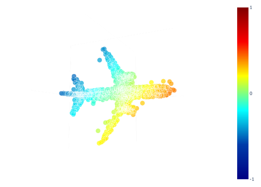
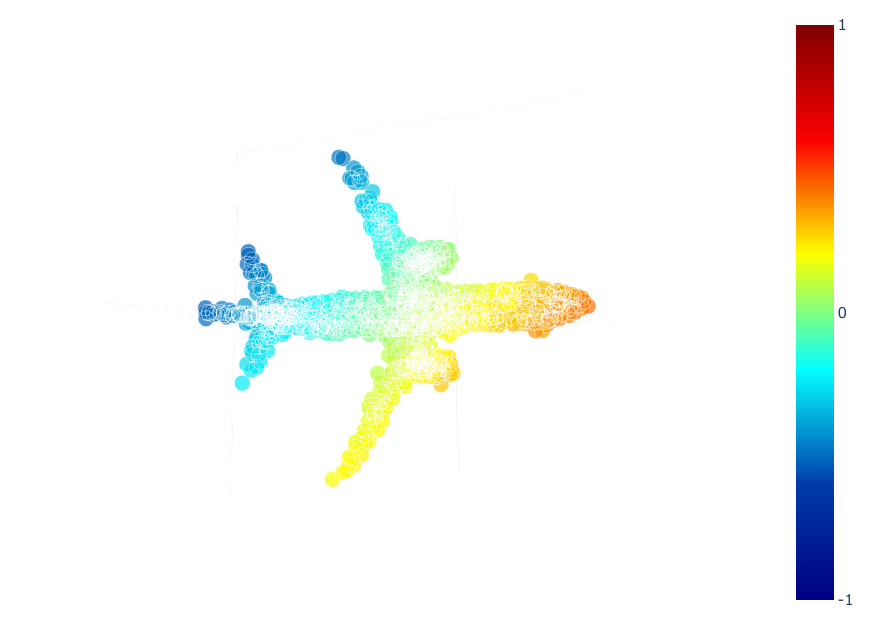
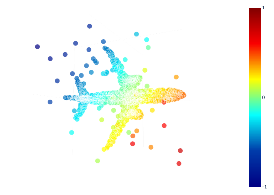
The visualization of our modified ModelNet40-C Sun et al. 2022 dataset with noise and outlier corruptions is demonstrated in Fig. 13.

References

- Aoki et al. [2019] Yasuhiro Aoki, Hunter Goforth, Rangaprasad Arun Srivatsan, and Simon Lucey. Pointnetlk: Robust & efficient point cloud registration using pointnet. In Proceedings of the IEEE/CVF conference on computer vision and pattern recognition, pages 7163–7172, 2019.
- Arora et al. [2019] Sanjeev Arora, Simon Du, Wei Hu, Zhiyuan Li, and Ruosong Wang. Fine-grained analysis of optimization and generalization for overparameterized two-layer neural networks. In International Conference on Machine Learning, pages 322–332. PMLR, 2019.
- Bietti and Mairal [2019] Alberto Bietti and Julien Mairal. On the inductive bias of neural tangent kernels. arXiv preprint arXiv:1905.12173, 2019.
- Bueno and Hylton [2021] Christian Bueno and Alan Hylton. On the representation power of set pooling networks. Advances in Neural Information Processing Systems, 34:17170–17182, 2021.
- Du et al. [2018] Simon S Du, Xiyu Zhai, Barnabas Poczos, and Aarti Singh. Gradient descent provably optimizes over-parameterized neural networks. arXiv preprint arXiv:1810.02054, 2018.
- Gould et al. [2019] Stephen Gould, Richard Hartley, and Dylan Campbell. Deep declarative networks: A new hope. arXiv preprint arXiv:1909.04866, 2019.
- Guo et al. [2021] Meng-Hao Guo, Jun-Xiong Cai, Zheng-Ning Liu, Tai-Jiang Mu, Ralph R Martin, and Shi-Min Hu. Pct: Point cloud transformer. Computational Visual Media, 7(2):187–199, 2021.
- Jacot et al. [2018] Arthur Jacot, Franck Gabriel, and Clément Hongler. Neural tangent kernel: Convergence and generalization in neural networks. arXiv preprint arXiv:1806.07572, 2018.
- Lee et al. [2019] Jaehoon Lee, Lechao Xiao, Samuel S Schoenholz, Yasaman Bahri, Roman Novak, Jascha Sohl-Dickstein, and Jeffrey Pennington. Wide neural networks of any depth evolve as linear models under gradient descent. arXiv preprint arXiv:1902.06720, 2019.
- Li et al. [2021] Xueqian Li, Jhony Kaesemodel Pontes, and Simon Lucey. Pointnetlk revisited. In Proceedings of the IEEE/CVF Conference on Computer Vision and Pattern Recognition, pages 12763–12772, 2021.
- Liu et al. [2019] Yongcheng Liu, Bin Fan, Shiming Xiang, and Chunhong Pan. Relation-shape convolutional neural network for point cloud analysis. In Proceedings of the IEEE/CVF Conference on Computer Vision and Pattern Recognition, pages 8895–8904, 2019.
- Mildenhall et al. [2020] Ben Mildenhall, Pratul P Srinivasan, Matthew Tancik, Jonathan T Barron, Ravi Ramamoorthi, and Ren Ng. Nerf: Representing scenes as neural radiance fields for view synthesis. In European Conference on Computer Vision, pages 405–421. Springer, 2020.
- Mildenhall et al. [2021] Ben Mildenhall, Pratul P Srinivasan, Matthew Tancik, Jonathan T Barron, Ravi Ramamoorthi, and Ren Ng. Nerf: Representing scenes as neural radiance fields for view synthesis. Communications of the ACM, 65(1):99–106, 2021.
- Mukhaimar et al. [2019] Ayman Mukhaimar, Ruwan Tennakoon, Chow Yin Lai, Reza Hoseinnezhad, and Alireza Bab-Hadiashar. Pl-net3d: robust 3d object class recognition using geometric models. IEEE Access, 7:163757–163766, 2019.
- Mukhaimar et al. [2021] Ayman Mukhaimar, Ruwan Tennakoon, Chow Yin Lai, Reza Hoseinnezhad, et al. Robust pooling through the data mode. arXiv preprint arXiv:2106.10850, 2021.
- Nguyen et al. [2015] Anh Nguyen, Jason Yosinski, and Jeff Clune. Deep neural networks are easily fooled: High confidence predictions for unrecognizable images. In Proceedings of the IEEE conference on computer vision and pattern recognition, pages 427–436, 2015.
- Qi et al. [2017a] Charles R Qi, Hao Su, Kaichun Mo, and Leonidas J Guibas. PointNet: Deep learning on point sets for 3D classification and segmentation. In CVPR, pages 652–660, 2017a.
- Qi et al. [2018] Charles R Qi, Wei Liu, Chenxia Wu, Hao Su, and Leonidas J Guibas. Frustum pointnets for 3d object detection from rgb-d data. In Proceedings of the IEEE conference on computer vision and pattern recognition, pages 918–927, 2018.
- Qi et al. [2017b] Charles Ruizhongtai Qi, Li Yi, Hao Su, and Leonidas J Guibas. Pointnet++: Deep hierarchical feature learning on point sets in a metric space. Advances in neural information processing systems, 30, 2017b.
- Rousseeuw and Leroy [2005] Peter J Rousseeuw and Annick M Leroy. Robust regression and outlier detection. John wiley & sons, 2005.
- Sanghi and Jayaraman [2020] Aditya Sanghi and Pradeep Kumar Jayaraman. How powerful are randomly initialized pointcloud set functions? arXiv preprint arXiv:2003.05410, 2020.
- Soelch et al. [2019] Maximilian Soelch, Adnan Akhundov, Patrick van der Smagt, and Justin Bayer. On deep set learning and the choice of aggregations. In International Conference on Artificial Neural Networks, pages 444–457. Springer, 2019.
- Stanley [2007] Kenneth O Stanley. Compositional pattern producing networks: A novel abstraction of development. Genetic programming and evolvable machines, 8(2):131–162, 2007.
- Sun et al. [2022] Jiachen Sun, Qingzhao Zhang, Bhavya Kailkhura, Zhiding Yu, Chaowei Xiao, and Z. Morley Mao. Benchmarking robustness of 3d point cloud recognition against common corruptions. arXiv preprint arXiv:2201.12296, 2022.
- Tancik et al. [2020] Matthew Tancik, Pratul P Srinivasan, Ben Mildenhall, Sara Fridovich-Keil, Nithin Raghavan, Utkarsh Singhal, Ravi Ramamoorthi, Jonathan T Barron, and Ren Ng. Fourier features let networks learn high frequency functions in low dimensional domains. arXiv preprint arXiv:2006.10739, 2020.
- Thomas et al. [2019] Hugues Thomas, Charles R Qi, Jean-Emmanuel Deschaud, Beatriz Marcotegui, François Goulette, and Leonidas J Guibas. Kpconv: Flexible and deformable convolution for point clouds. In Proceedings of the IEEE/CVF international conference on computer vision, pages 6411–6420, 2019.
- Vaswani et al. [2017] Ashish Vaswani, Noam Shazeer, Niki Parmar, Jakob Uszkoreit, Llion Jones, Aidan N Gomez, Łukasz Kaiser, and Illia Polosukhin. Attention is all you need. Advances in neural information processing systems, 30, 2017.
- Wang et al. [2019] Yue Wang, Yongbin Sun, Ziwei Liu, Sanjay E Sarma, Michael M Bronstein, and Justin M Solomon. Dynamic graph cnn for learning on point clouds. Acm Transactions On Graphics (tog), 38(5):1–12, 2019.
- Wu et al. [2019] Wenxuan Wu, Zhongang Qi, and Li Fuxin. Pointconv: Deep convolutional networks on 3d point clouds. In Proceedings of the IEEE/CVF Conference on computer vision and pattern recognition, pages 9621–9630, 2019.
- Wu et al. [2015] Zhirong Wu, Shuran Song, Aditya Khosla, Fisher Yu, Linguang Zhang, Xiaoou Tang, and Jianxiong Xiao. 3d shapenets: A deep representation for volumetric shapes. In Proceedings of the IEEE conference on computer vision and pattern recognition, pages 1912–1920, 2015.
- Zaheer et al. [2017] Manzil Zaheer, Satwik Kottur, Siamak Ravanbakhsh, Barnabas Poczos, Russ R Salakhutdinov, and Alexander J Smola. Deep sets. Advances in neural information processing systems, 30, 2017.
- Zhao et al. [2021] Hengshuang Zhao, Li Jiang, Jiaya Jia, Philip HS Torr, and Vladlen Koltun. Point transformer. In Proceedings of the IEEE/CVF international conference on computer vision, pages 16259–16268, 2021.
- Zheng et al. [2021] Jianqiao Zheng, Sameera Ramasinghe, and Simon Lucey. Rethinking positional encoding. arXiv preprint arXiv:2107.02561, 2021.
- Zheng et al. [2022] Jianqiao Zheng, Sameera Ramasinghe, Xueqian Li, and Simon Lucey. Trading positional complexity vs deepness in coordinate networks. In European Conference on Computer Vision, pages 144–160. Springer, 2022.
- Zhong et al. [2019] Ellen D Zhong, Tristan Bepler, Joseph H Davis, and Bonnie Berger. Reconstructing continuous distributions of 3d protein structure from cryo-em images. arXiv preprint arXiv:1909.05215, 2019.
Supplementary Material
We provide additional details of our method and experiments in the supplementary material.
7 RFF Derivation
In this section, we extend the derivation of Random Fourier Features (RFF) from band-limited embeddings discussed in the main text Sec. 3.1. In particular,
- 1.
We derive a per-point embedding (PPE) not trained on data that is better for out-of-domain (OOD) generalization.
- 2.
Empirically, sinusoidal embeddings are better than ReLU embeddings under randomly initialized conditions. This finding can be explained by the tradeoff between the controllable bandwidth and the local smoothness.
- 3.
We show why RFF is a band-limited PE and derive RFF from sinusoidal embeddings. Since RFF is a derivative of sinusoidal embeddings, it explains why it is a more robust PPE than other band-limited PEs.