HIGH-PRECISION OBSERVABLE ESTIMATION WITH SINGLE QUBIT QUANTUM MEMORY

Determining the expectation value of multi-qubit observables within a quantum system is a fundamental subject in numerous domains of quantum science. Notably, in condensed matter physics, materials science, quantum chemistry, and combinatorial optimization [1], the objective revolves around identifying spectral characteristics, such as the ground state energy or the lowest eigenvalue of a Hamiltonian. However, the direct estimation of the observable expectation value is not a straightforward task in these scenarios. The quantum phase estimation (QPE) algorithm [2, 3, 4, 5, 6, 7], offers a potential solution for ideal quantum processing units with extended coherence times. However, in the Noisy Intermediate-Scale Quantum (NISQ) era, QPE’s implementation is hindered by coherence time limitations. To overcome this, the quantum energy (expectation) estimation (QEE) method is widely used, especially within the variational quantum eigensolver framework [8].

QEE requires just single qubit measurements and thus a minimum coherence time of the quantum device. However, it is not without its limitations. One such drawback is the accumulation of shot noise during the estimation process, which leads to a reduction in the overall variance level. In QEE, the individual Pauli strings are estimated separately, and subsequently, a linear combination of these estimates is utilized to determine the value of the observable.

Consequently, in order to estimate an observable comprised of $N$ Pauli strings with a variance of $\eta$, each Pauli string should be estimated with an variance of $O(\eta/N)$. The resulting sample complexity therefore scales as $O(N^{2})$. This can pose a significant challenge since the total number of measurements will eventually be limited by the available run-time of the quantum device. It is important to note that the measurement process itself is often one of the most time-consuming operations in current quantum devices [9, 10, 11].

Recent studies have proposed strategies to minimize sample complexity by aggregating commuting sets of Pauli strings [12, 13, 14], serving as alternatives between QPE and QEE. While these approaches improve efficiency and reduce quantum resource requirements for obtaining the observable’s expectation value, they face challenges. Notably, they do not address the fundamental scaling issue related to noise accumulation with the increasing number of Pauli strings in the observable decomposition [15, 14].

In our recent paper [16], we introduced a novel algorithm known as the Coherent Pauli Summation (CPS) method, which effectively mitigates the issue of shot-noise accumulation by leveraging a single-qubit quantum memory (QM). The pivotal aspect of the CPS method lies in the utilization of Quantum Signal Processing (QSP) techniques [17], to encode the mean value of Pauli strings within the phase of a single qubit QM. By circumventing the accumulation of shot noise, the CPS method achieves a significant improvement in the variance of the estimate compared to the Quantum Energy Estimation (QEE) method, scaling at $O(N)$, where $N$ is the number of Pauli strings in the observable decomposition. However, the QSP step necessitates multiple controlled many-qubit unitaries between the single qubit quantum memory and the many-qubit NISQ device for the encoding of each Pauli string. This can have a detrimental effect on the coherence of the quantum memory given the complexity of such operations. In general, it is desirable to limit the number of interactions with the quantum memory as much as possible to uphold the coherence of the stored information.

A single-qubit QM typically consists of a physical system, such as an individual ion [18, 19] or Rydberg atom [20], capable of storing and maintaining the quantum state of a qubit. Such QM performs well while isolated from the environment to have low decoherence rates and long coherence times to preserve information. Another possibility is an error-corrected QM [21, 22]. Its basic idea is to use a larger number of physical qubits to represent each logical qubit. These physical qubits are entangled with each other and form an error-correcting code, which allows the system to detect and correct errors without losing the encoded quantum information. Even if some of the physical qubits experience errors, the encoded logical qubit can be recovered with high fidelity. While error-corrected QM holds significant promise in mitigating errors and enhancing the reliability of quantum information processing, it also comes with several disadvantages like increasing complexity and reducing the processing speed. Moreover, the process of error correction itself introduces a possibility of logical errors due to imperfect gate operations or residual errors in the encoding. The CPS requires $N\log{(N/\sqrt{\eta})}/\log{(\log{(N/\sqrt{\eta})})}$ controlled unitary operations between the NISQ qubits and the memory qubit that is a challenging demand for the current QMs.

In this article, we present an alternative approach to our CPS method. Instead of relying on QSP techniques for encoding the mean value of Pauli strings in the phase, we propose the utilization of a Taylor series approach. By employing the Taylor-based CPS method (TCPS), we achieve a variance improvement of the final estimate compared to the QEE method, scaling as $N^{2/3}$. While the coherence time of the memory qubit required for both TCPS and the original CPS method scales linearly with $N$, the TCPS method only requires a single controlled unitary between the memory qubit and the multi-qubit device for the encoding of a Pauli string compared to the $O(\log(1/\eta))$ number of unitaries required for the CPS method, where $\eta$ is the target precision of final multi-qubit observable estimate. Although the TCPS approach exhibits a slight scaling disadvantage compared to the original CPS method, it offers the advantage of fewer interactions between the single qubit memory and the multi-qubit device which can important for practical implementations.

The paper is organised as follows. In Section 1 we briefly outline the QEE method. In Section 2 the TCPS method is studied in details. We compare it with the QEE method in terms of variance of the resulting estimate and the resources. All technical details are given in Appendix.

We start by going through the main steps of the QEE technique. Decomposition of an observable $O$ into a weighted sum of Pauli strings

is a crucial step in the QEE for determining the expected value of a given observable for a particular quantum state $\ket{\Psi}$. Here $a_{j}\in R$ are the decomposition coefficients and $P_{j}$ are the Pauli strings composed as tensor products of single qubit Pauli matrices and the identity. Since a set of $d^{2}$ Pauli strings form a complete operator basis for a Hilbert space with dimension $d$ this decomposition is always possible.

The Pauli strings are measured sequentially or in parallel (if the strings are commuting), using single qubit projective measurements in order to provide an estimate of each Pauli string $\langle P_{j}\rangle\equiv\langle\Psi|P_{j}|\Psi\rangle$ [8, 23]. The mean value of the observable $O$ is than calculated by the classical summation of the later estimates (see Fig. 1):

It follows that the shot noise from the individually estimated mean values of the Pauli strings accumulates in the final estimate of $\langle O\rangle$. If every $\langle P_{j}\rangle$ is estimated with a variance $\sigma^{2}(\langle\hat{P}_{j}\rangle)$ then, assuming equal weights of the Pauli strings in (1), the variance of estimate of $O$ is $\sigma^{2}(\hat{\langle O\rangle})\sim N\sigma^{2}(\langle\hat{P}_{j}\rangle)$.

Since the dimension of the Hilbert space increases exponentially with the number of qubits, the number of Pauli stings $N$ in the decomposition (1) can be very large. In particular, the encoding of fermionic Hamiltonians in a qubit lattice poses a problem for quantum simulators of fermionic systems. In [24], local fermionic Hamiltonian systems are mapped to local spin Hamiltonians (fermion-to-qubit mapping) suitable for analog quantum simulation applications. However, such transformations introduce long-range many-body interaction terms, which are beyond the scope of the current implementation and necessitate special reduction algorithms [25].

To overcome the accumulation of shot noise we employ phase-kick back techniques to encode the mean value of each Pauli string into the phase of a single qubit QM, allowing the encoding of $\langle O\rangle$ which can be directly measured.

Let $|\Psi_{0}\rangle\equiv V|\boldsymbol{0}\rangle$ be a quantum state of the NISQ device, where $V$ is an invertible preparation circuit. By $|\boldsymbol{0}\rangle$ we denote the state where all qubits are prepared in their ground states $\ket{0}$. Our target is to estimate the expectation value $\langle\Psi_{0}|O|\Psi_{0}\rangle$ with a variance of $\eta$. To this end, we define $|\Psi_{1}\rangle_{j}\equiv P_{j}|\Psi_{0}\rangle$ and introduce the unitary operator

where $\Pi_{0}=I-2\ket{\boldsymbol{0}}\bra{\boldsymbol{0}}$ is a projector, and $I$ is the identity operator. This operator defines a rotation by a principal angle

between two closed subspaces $|\Psi_{0}\rangle$ and $|\Psi_{j}\rangle$ of a Hilbert space. It holds that the state $|\Psi_{0}\rangle$ is an equal superposition of eigenstates $|\phi^{\pm}\rangle$ of $U_{P_{j}}$ with eigenvalues $e^{\pm i\phi}$, respectively [26, 12].

We introduce the state

where the first register describes the processing ancillary. Acting on this state with a unitary operator $|0\rangle_{p}\langle 0|\otimes I+|1\rangle_{p}\langle 1|\otimes cP_{j}$, we get the following $\epsilon^{\prime}$-dependent state

Let us introduce $|\tilde{\Psi}_{1}\rangle\equiv(\sigma_{x}\otimes I)|\tilde{\Psi}_{0}\rangle$ and calculate the overlap

To encode the weighted sum of the Pauli strings we select $\sqrt{\epsilon^{\prime}_{j}(1-\epsilon^{\prime}_{j})}\equiv|a_{j}|\sqrt{\epsilon}$, where the parameter $\epsilon\in(0,1)$, holds.

The rotation operators $(\tilde{U})_{P_{j}}(\epsilon)=\tilde{V}\Pi_{0}\tilde{V}^{\dagger}P_{j}$, $\tilde{V}(P_{j}):\tilde{V}(P_{j})|0\rangle=|\tilde{\Psi}_{0}\rangle_{j}$ can be introduced to encode the Pauli strings in the phases. The operator $(\tilde{U})_{P_{j}}(\epsilon)$ defines the rotation by a principal angle

between two closed subspaces $|\tilde{\Psi}_{0}\rangle$ and $|\tilde{\Psi}_{1}\rangle$ of a Hilbert space. Since this encoding method requires preparation of the eigenstates $|\phi^{\pm}\rangle$ of the rotation operators at each iteration, it is important to mention, that we can write $|\tilde{\Psi}_{0}\rangle$ as a superposition

Hence, projecting on $|\tilde{\phi}_{0}^{\pm}\rangle$ states is equivalent to projecting on $|\phi^{\pm}\rangle$, respectively.

To encode the information about the mean value of the Pauli string in the phase we define a memory qubit in the state $\ket{\psi}_{m}=\ket{+}_{m}$. The controlled version c$(\tilde{U})_{P_{j}}(\epsilon)$ can be implemented by substituting $P_{j}$ with its controlled version, c$P_{j}$. Applying c$(\tilde{U})_{P_{j}}(\epsilon)$ to the state $\ket{\psi}_{m}|\tilde{\Psi}_{0}\rangle$, we get

with the information about the mean value of the Pauli string encoded in the phase, i.e.

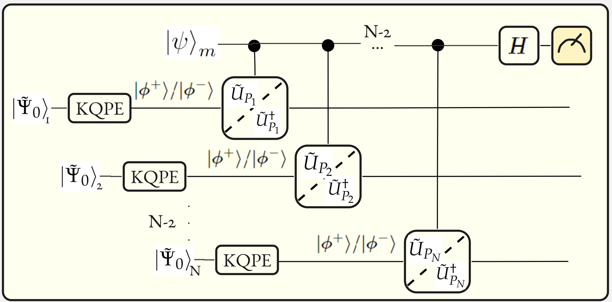
Using this encoding method, we can encode the correct linear combination of the $N$ mean values of Pauli strings sequentially in the phase of the memory qubit as depicted in Fig. 2. The final state of the memory qubit will be $(|0\rangle+e^{i\tilde{\Phi}}|1\rangle)/\sqrt{2}$, where

Finally, we perform a projective measurement on the QM qubit to estimate the phase following the standard Kitaev phase estimation procedure [2]. To obtain a good estimate of $\tilde{\Phi}$, the whole encoding process and measurement process is repeated $M_{q}$ times.

The complication arise from the fact, that since $|\tilde{\Psi}_{0}\rangle$ is an equal superposition of $|\phi^{\pm}\rangle$ and $\cos{(\cdot)}$ is an even function, we need to project onto one of the eigenstates $|\phi^{+}\rangle$ or $|\phi^{-}\rangle$ prior to encoding to control the sing of the phase. Note that both eigenstates work since the sign can be controlled by using either $(\tilde{U})_{P_{j}}(\epsilon)$ or $(\tilde{U})^{\dagger}_{P_{j}}(\epsilon)$, depending on the eigenstate projection. This is necessary since the end goal is to encode a given linear combination of Pauli strings in the phase of the memory qubit through sequential application of the encoding step with different Pauli strings, $P_{j}$.

To perform the eigenstate projection, a small series of partial projections (Kitaev’s quantum phase estimation (KQPE) steps [2]) are performed prior to the encoding to efficiently resolve between $|\phi^{+}\rangle$ and $|\phi^{-}\rangle$. This can be achieved using an auxiliary qubit as the control qubit [12] instead of the memory qubit. It suffices to do enough measurements to accurately determine the sign of the encoded phase in the auxiliary qubit while the actual phase is not necessary to estimate. Consequently, this can be done efficiently with the total number of QPE steps, $n_{QPE}$, scaling logarithmic with the total number of Pauli strings to be encoded assuming that the mean value of each Pauli string is bounded away from zero. For details, we refer to the Appendices B-D. Importantly, the eigenstate projection is performed using an additional auxiliary qubit and not the memory qubit. This is what allows us to reduce the interactions between the memory qubit and the many-qubit device compared to the CPS method.

The steps of our method are the following (see Fig. 1):

• •

  First, we roughly estimate the mean values of every Pauli string $\langle\Psi_{0}|P_{j}|\Psi_{0}\rangle$, $j=\overline{1,N}$ by a small series of projective measurements like it is done in the QEE method. This step provides information about the sign and magnitude (bounded away from zero) of the mean values of the Pauli strings. For more details see Appendix B.

• •

  Second, for every $P_{j}$ (that is bounded away from zero), we do $n_{QPE}$ of KQPE steps on $|\tilde{\Psi}_{0}\rangle$, projecting on either $|\phi^{+}\rangle$ and $|\phi^{-}\rangle$. If we project on $|\phi^{+}\rangle$, we encode the mean value the Pauli string in the phase of the memory qubit using $c(\tilde{U})_{P_{j}}(\epsilon)$ while for $|\phi^{-}\rangle$, we use $c(\tilde{U})^{\dagger}_{P_{j}}(\epsilon)$. For more details see Appendix C.

For $\epsilon\ll\,1$, the Taylor expansion is used to rewrite Eq. (12). To lowest order in $\epsilon$, we get:

The error due to higher order terms in $\epsilon$ can, however, be corrected using additional information from the rough estimates of the mean values used to estimate the signs and magnitudes of the Pauli strings. In Appendices D-E, the correction procedure is described in detail and the final variance of the estimate $\hat{O}$ is deduced assuming that $M_{c}^{cor}$ projective measurements are used for the rough estimates. The variance of the corrected estimate scales as $\sigma^{2}{(\hat{O}^{TCPS})}\sim N^{\frac{4}{3}}T^{-1}$, where $T$ is the total amount of controlled unitaries used in the TCPS method. This scaling results as a trade-off between the inaccuracy of the estimate due to the Taylor expansion and the added noise from the correction procedure.

Note that in our method, the phase estimation is limited to the modulus of $2\pi$. To address the issue of phase wrapping, we adopt the sampling approach introduced in [27, 3]. Instead of encoding $\phi$ with a fixed $\epsilon$, we employ multiple orders of sampling, denoted as $\tilde{\epsilon}_{l}\equiv 2^{l}\sqrt{\epsilon_{0}}$, where $l=1,2,\dots,d_{L}$, to gradually zoom in on the value of $\phi$. By appropriately selecting $d_{L}$ and the total number of measurement repetitions, we achieve the same variance rate. The initial parameter $\epsilon_{0}$ is chosen in such a way that $\tilde{\Phi}(\epsilon_{0})<2\pi$ holds. Further detailed analyses and discussions can be found in Appendix G.

We performed a comprehensive comparison of resources between the TCPS, the QEE and CPS, as detailed in Table 1. The number of state preparation circuits required and the coherence time of the necessary processing ancillas are compared. To implement $\tilde{U}_{P_{j}}(\epsilon)$ in the TCPS technique, the controlled sign flip operator $\Pi_{0}$ and two state preparation circuits $\tilde{V}$ and $\tilde{V}^{\dagger}$ are needed. The controlled $\Pi_{0}$ can be implemented using a series of two-qubit CNOT gates, which scales linearly with the number of qubits in the NISQ device [12, 28] and we therefore view this as having the same cost as the state preparation circuit.

In terms of time consumption, the state preparation step $t_{prep}$ is considered the most time-consuming, which is also used to quantify the time of the encoding operations. In the QEE method, the coherence time of the NISQ device is $t_{prep}$ as each qubit is measured after each state preparation. On the other hand, the TCPS method necessitates a modest increase in the coherence time of the NISQ device. This increase scales logarithmically with the number of Pauli strings and the target variance $\eta$. Additionally, the TCPS method relies on a long coherence time memory qubit, whose coherence time is linearly dependent on the number of Pauli strings $N$. In cases where the available resources cannot provide the required coherence time, the total Pauli sum must be divided into sub-sums and encoded in QM separately.

In return, the TCPS method provides a much better estimate of $\langle O\rangle$ than the QEE method for a fixed number of state preparations. Comparing it with the variance of QEE method in the case of equal amount of resources used in both methods, we get

which shows that the TCPS method achieves a better scaling of the variance in the number of Pauli strings compared to the scaling of the QEE approach.

As we mentioned in [16] both the QEE and CPS methods are subject to the accumulation of operational errors, which poses a limitation on the accuracy of the final estimate of the observable. The presence of gate errors significantly affects the reliability of both approaches, ultimately impacting the quality of the observables estimation. However, in contrast to the CPS, the TCPS method has less interactions of the NISQ qubits with the QM. In TCPS method the encoding of every Pauli string in the QM is done by only one unitary gate. That means, that the amount of operations between NISQ qubits and the QM is $N$ that is significantly less then in the CPS method. This fact makes TCPS method more robust to the QM corruption due to the interactions, however in terms of robustness to gate errors the TCPS and the CPS are similar.

We proposed an alternative variation of our Coherent Pauli Summation method recently provided in [16] called the Taylor Coherent Pauli Summation method to estimate the expectation values of multi-qubit observables. The method uses phase-kick back techniques and Taylor decomposition to encode information from a multi-qubit processor into a single qubit quantum memory. In this way the accumulation of the shot noise that arise in the conventional QEE approach is avoided. The variance of the TCPS method outperforms the QEE approach as $\sim 1/N^{2/3}$. For observables with a large Pauli string decomposition our method gives a significant advantage, especially if there are many non-commuting Pauli sets. If the Pauli stings can be efficiently sorted in commuting sets they could be measured in parallel using the QEE method while the TCPS method in the current form in not parallelizable. Thus, our method can be combined with known QEE approaches and applied in cases where sorting into commuting sets is hard (in general it is NP hard) or simply not possible.

In comparison to the CPS, TCPS approach exhibits slightly higher variance but is more robust to the logical errors of the QM. We have demonstrated that TCPS demands $N$ controlled unitary interactions of the NISQ qubits with the QM, making it more experimentally feasible on NISQ devices then CPS.

L.M. was partly supported by the Netherlands Organisation for Scientific Research (NWO/OCW), as part of the Quantum Software Consortium program (project number 024.003.037 / 3368). This research work was partly supported by the Roadmap for the Development of Quantum Technologies in Russian Federation, contract No. 868-1.3-15/15-2021.

References

- [1] G.H. Golub and H.A. van der Vorst. Eigenvalue computation in the 20th century. J. Comput. Appl. Math, 123(1):35–65, 2000. Numerical Analysis 2000. Vol. III: Linear Algebra.
- [2] A. Yu. Kitaev. Quantum measurements and the abelian stabilizer problem. Conferance, 1995.
- [3] S. Kimmel, G.H. Low, and T.J. Yoder. Robust calibration of a universal single-qubit gate set via robust phase estimation. Phys. Rev. A, 92:062315, 2015.
- [4] E. van den Berg. Iterative quantum phase estimation with optimized sample complexity. In 2020 IEEE International Conference on Quantum Computing and Engineering (QCE), pages 1–10, 2020.
- [5] H. Mohammadbagherpoor, Y.H. Oh, P. Dreher, A. Singh, X. Yu, and A.J. Rindos. An improved implementation approach for quantum phase estimation on quantum computers. In 2019 IEEE International Conference on Rebooting Computing (ICRC), pages 1–9. IEEE, 2019.
- [6] N. Wiebe and C. Granade. Efficient bayesian phase estimation. Phys. Rev. Lett., 117:010503, Jun 2016.
- [7] T.E. O’Brien, B. Tarasinski, and B.M. Terhal. Quantum phase estimation of multiple eigenvalues for small-scale (noisy) experiments. New J. Phys, 21(2):023022, feb 2019.
- [8] A. Peruzzo, J. McClean, P. Shadbolt, M.-H. Yung, X.-Q. Zhou, P.J. Love, A. Aspuru-Guzik, and J.L. O’Brien. A variational eigenvalue solver on a photonic quantum processor. Nat. Commun, 5, 2014.
- [9] P. Jurcevic, A. Javadi-Abhari, L.S. Bishop, I. Lauer, D.F. Bogorin, M. Brink, L. Capelluto, O. Günlük, T. Itoko, N. Kanazawa, et al. Demonstration of quantum volume 64 on a superconducting quantum computing system. Quantum Sci. Technol., 6(2):025020, 2021.
- [10] K.R. Brown, J. Kim, and C. Monroe. Co-designing a scalable quantum computer with trapped atomic ions. npj Quantum Inf., 2(1):1–10, 2016.
- [11] V.M. Schäfer, C.J. Ballance, K. Thirumalai, L.J. Stephenson, T.G. Ballance, A.M. Steane, and D.M. Lucas. Fast quantum logic gates with trapped-ion qubits. Nature, 555(7694):75–78, 2018.
- [12] D. Wang, O. Higgott, and S. Brierley. Accelerated variational quantum eigensolver. Phys. Rev. Lett., 122:140504, Apr 2019.
- [13] I. Hamamura and T. Imamichi. Efficient evaluation of quantum observables using entangled measurements. npj Quantum Inf., 6:2056–6387, 2020.
- [14] O. Crawford, B. Straaten, D. Wang, T. Parks, E. Campbell, and S. Brierley. Efficient quantum measurement of Pauli operators in the presence of finite sampling error. Quantum, 5:385, January 2021.
- [15] J. R. McClean, J. Romero, R. Babbush, and A. Aspuru-Guzik. The theory of variational hybrid quantum-classical algorithms. New J. Phys, 18(2):023023, feb 2016.
- [16] L.A. Markovich, A. Almasi, S. Zeytinoglu, and J. Borregaard. Quantum memory assisted observable estimation, 2022.
- [17] G.H. Low and I.L. Chuang. Optimal hamiltonian simulation by quantum signal processing. Phys. Rev. Lett., 118:010501, Jan 2017.
- [18] C. Langer, R. Ozeri, J.D. Jost, J. Chiaverini, B. DeMarco, A. Ben-Kish, R.B. Blakestad, J. Britton, D.B. Hume, W.M. Itano, et al. Long-lived qubit memory using atomic ions. Phys. rev. lett., 95(6):060502, 2005.
- [19] Y. Wang, M. Um, J. Zhang, S. An, M. Lyu, J.-N. Zhang, L.-M. Duan, D. Yum, and K. Kim. Single-qubit quantum memory exceeding ten-minute coherence time. Nature Phot., 11(10):646–650, 2017.
- [20] L. Li and A. Kuzmich. Quantum memory with strong and controllable rydberg-level interactions. Nat. Comm., 7(1):13618, 2016.
- [21] B.M. Terhal. Quantum error correction for quantum memories. Rev. Mod. Phys., 87:307–346, Apr 2015.
- [22] J.R. Wootton. Quantum memories and error correction. Journal of Modern Optics, 59(20):1717–1738, 2012.
- [23] J. R. McClean, R. Babbush, P. J. Love, and A. Aspuru-Guzik. Exploiting locality in quantum computation for quantum chemistry. J. Phys. Chem. Lett, 5(24):4368–4380, 2014. PMID: 26273989.
- [24] Pascual Jordan and Eugene Paul Wigner. Über das paulische äquivalenzverbot. In The Collected Works of Eugene Paul Wigner, pages 109–129. Springer, 1993.
- [25] Panagiotis Kl. Barkoutsos, Nikolaj Moll, Peter W. J. Staar, Peter Mueller, Andreas Fuhrer, Stefan Filipp, Matthias Troyer, and Ivano Tavernelli. Fermionic hamiltonians for quantum simulations: a general reduction scheme, 2017.
- [26] E. Knill, G. Ortiz, and R. D. Somma. Optimal quantum measurements of expectation values of observables. Phys. Rev. A, 75:012328, Jan 2007.
- [27] B.L. Higgins, D.W. Berry, S.D. Bartlett, M.W. Mitchell, H.M. Wiseman, and G.J. Pryde. Demonstrating heisenberg-limited unambiguous phase estimation without adaptive measurements. New J. Phys, 11(7):073023, jul 2009.
- [28] D. Maslov. Advantages of using relative-phase toffoli gates with an application to multiple control toffoli optimization. Phys. Rev. A, 93:022311, Feb 2016.
- [29] S. Gulde, M. Riebe, G.P.T. Lancaster, C. Becher, J. Eschner, H. Häffner, F. Schmidt-Kaler, I.L. Chuang, and R. Blatt. Implementation of the deutsch–jozsa algorithm on an ion-trap quantum computer. Nature, 421(6918):48–50, 2003.
- [30] C. Monroe and J. Kim. Scaling the ion trap quantum processor. Science, 339(6124):1164–1169, 2013.
- [31] K. Mølmer, L. Isenhower, and M. Saffman. Efficient grover search with rydberg blockade. J. Phys. B: At. Mol. Opt. Phys, 44(18):184016, 2011.
- [32] L. Isenhower, M. Saffman, and K. Mølmer. Multibit c k not quantum gates via rydberg blockade. Quantum Inf. Process., 10:755–770, 2011.
- [33] P. Wang, C.-Y. Luan, M. Qiao, M. Um, J. Zhang, Y. Wang, X. Yuan, M. Gu, J. Zhang, and K. Kim. Single ion qubit with estimated coherence time exceeding one hour. Nature communications, 12(1):233, 2021.
- [34] A.H. Myerson, S.C. Szwer, D.J.and Webster, D.T.C. Allcock, M.J. Curtis, G. Imreh, J.A. Sherman, D.N. Stacey, A.M. Steane, and D.M. Lucas. High-fidelity readout of trapped-ion qubits. Phys. Rev. Lett., 100(20):200502, 2008.
- [35] S. Crain, C. Cahall, G. Vrijsen, E.E. Wollman, M.D. Shaw, V.B. Verma, S.W. Nam, and J. Kim. High-speed low-crosstalk detection of a 171yb+ qubit using superconducting nanowire single photon detectors. Comm. Phys., 2(1):97, 2019.
- [36] Z. Cai, C.-Y. Luan, L. Ou, H. Tu, Z. Yin, J.-N. Zhang, and K. Kim. Entangling gates for trapped-ion quantum computation and quantum simulation. Journal of the Korean Physical Society, pages 1–19, 2023.
- [37] C.R. Clark, H.N. Tinkey, B.C. Sawyer, A.M. Meier, K. A. Burkhardt, C.M. Seck, C.M. Shappert, N.D. Guise, C.E. Volin, S.D. Fallek, H.T. Hayden, W.G. Rellergert, and K.R. Brown. High-fidelity bell-state preparation with optical qubits. Phys. Rev. Lett., 127:130505, Sep 2021.
- [38] V.M. Schäfer, C.J. Ballance, K. Thirumalai, L.J. Stephenson, T.G. Ballance, A.M. Steane, and D.M. Lucas. Fast quantum logic gates with trapped-ion qubits. Nature, 555(7694):75–78, 2018.
- [39] J. Ramette, J. Sinclair, Z. Vendeiro, A. Rudelis, M. Cetina, and V. Vuletić. Any-to-any connected cavity-mediated architecture for quantum computing with trapped ions or rydberg arrays. PRX Quantum, 3:010344, Mar 2022.