Complex quantum momentum due to correlationPreprint: APS/123-QED
Abstract
Real numbers provide a sufficient description of classical physics and all measurable phenomena; however, complex numbers are occasionally utilized as a convenient mathematical tool to aid our calculations. On the other hand, the formalism of quantum mechanics integrates complex numbers within its fundamental principles, and whether this arises out of necessity or not is an important question that many have attempted to answer. Here, we will consider two electrons in a one-dimensional quantum well where the interaction potential between the two electrons is attractive as opposed to the usual repulsive coulomb potential. Pairs of electrons exhibiting such effective attraction towards each other occur in other settings, namely within superconductivity. We will demonstrate that this attractive interaction leads to the necessity of complex momentum solutions, which further emphasizes the significance of complex numbers in quantum theory. The complex momentum solutions are solved using a perturbative analysis approach in tandem with Newton’s method. The probability densities arising from these complex momentum solutions allow for a comparison with the probability densities of the typical real momentum solutions occurring from the standard repulsive interaction potential.
I Introduction
The prevalence of complex numbers throughout the quantum mechanic’s formalism is apparent within its fundamentals. The Schrödinger equation, wave functions, quantum operators, and commutation relations, to name a few, all employ its use extensively Chen et al. 2022. Although complex numbers are a useful mathematical tool, physical meaning is attributed solely to real quantities (e.g., real eigenvalues to represent an observable and modulus squared of the wave function for probability), while complex quantities are thought of as non-physical Karam 2020. Whether complex numbers are necessary for quantum mechanics or if real numbers alone provide a complete description is a topic that many have explored Miller 2022; Chen et al. 2022; Karam 2020; Renou et al. 2021; Li et al. 2022; Aleksandrova et al. 2013; Baez 2012; Myrheim 1999. Beginning with von Neumann in 1936 Chen et al. 2022; Bednorz and Batle 2022; Birkhoff and Neumann 1936, numerous works have demonstrated the ability to simulate quantum systems based only on real numbers using an extended Hilbert space Stueckelberg 1960; Guenin and Stueckelberg 1961; McKague et al. 2009. Conversely, in 2021, Renou et al. designed a Bell-like experiment that is potentially unexplainable by real quantum theory, hence providing compelling evidence towards the requirement of complex quantum theory for a complete explanation Renou et al. 2021. First, defining quantum theory upon four postulates Ismael 2021; Piron 1964, the entanglement-swapping ZUKOWSKI et al. 1993 experiment comprised of three observers: Alice, Bob, and Charlie, as shown in Fig. 1. Two pairs of maximally entangled qubits and as well as and are generated from different sources. The first qubit pair and are sent to Alice and Bob, respectively, while the second pair and are given to Bob and Charlie, respectively. A spin qubit consists of a two-dimensional complex vector Miller 2022, which means that when Bob performs a joint measurement on the qubits and , there are four possible outcomes. Once Bob performs this measurement, the entanglement between the pairs of qubits shifts to qubits and The new entangled qubit state between Alice and Charlie must maximally violate the CHSH3 inequality with a value of Renou et al. 2021, which is an amalgamation of three CHSH inequalities Acín et al. 2015; Bowles et al. 2018. Shortly after, two groups performed the proposed experiment observing results that supported the necessity of complex quantum theory Li et al. 2022; Chen et al. 2022. This work will further exemplify the indispensability of complex numbers in quantum mechanics, particularly the need for complex momentum solutions when considering two electrons confined in a one-dimensional quantum well with an attractive effective interaction potential between the two electrons. A first exposure to quantum mechanics typically starts with the problem of a single electron confined within a one-dimensional quantum well of length , in which the momentum solutions are found to be and Griffiths and Schroeter 2019. The consideration of two interacting electrons usually involves a repulsive interaction potential resulting in real momentum solutions. However, other works have considered complex momentum solutions, but in the context of two free bosonic particles Franchini 2011 or within the one-dimensional Heisenberg model Karle 2021; Bethe 1931.

II Model and analysis
Our model consists of two identical electrons, each with mass , confined in a one-dimensional quantum well of length . The Hamiltonian used to describe these two electrons within the well is given by:
| (1) |
where and are the position vectors of the two electrons and . The interaction potential between the two electrons was chosen to be pointlike, taking the form of a function, also known as the shape-independent approximation Busch et al. 1998. The function model was introduced by Frost Weber 1964 and it allows us to avoid any complications of the Coulomb potential, while still being able to emphasize the necessity of complex momentum solutions. If we were to consider a spin triplet state with an antisymmetrical spatial factor of the wave function, this would lead to the same wavefunction that comes about from the non-interacting case and is given by:
| (2) |
where and and . We can see that the delta interaction potential plays no role, and the momentum solutions remain real. As outlined in the Supplemental Material (SM) Sup, we will now consider a singlet state formed by the two electron spins, the Pauli exclusion principle requires a symmetrical spatial factor of the wave function Sakurai and Napolitano 2017. Consequently, this leads to a wavefunction of the form:
| (3) |
where and are normalization constants to be determined. The center-of-mass coordinate and the relative coordinate Busch et al. 1998 allow the Hamiltonian to be rewritten as:
| (4) |
In the region the Schrödinger equation gives:
| (5) |
In the usual way, we can integrate the Schrödinger equation from to in the limit Weber 1964
| (6) |
After some algebra and redefining and to be dimensionless quantities, we obtain two cases, in which each case has two corresponding equations that the solutions and must satisfy. The first case is when which has the two equations:
| (7) |
The second case where , which gives the two equations:
| (8) |
A comparison with the non-interacting case leads one to expect and solutions of Eq. (7) and (8) to lie in the neighborhood and where and are positive integers. Momentum solutions satisfying Eq. (7) require and to be of the same parity, while those satisfying Eq. (8) are required to be of different parity. If we let and and perform a perturbative analysis (see the SM Sup) around the region where that is and we obtain:
| (9) |
| (10) |
If the interaction potential between the two electrons is repulsive and we expect to find solutions where and are real. However, it is more interesting if we consider the interaction potential will be attractive and we expect the two electrons to have some binding tendencies. The effective attraction between two electrons has been seen within the context of superconductivity where in a metal, two electrons are attracted to each other forming a Cooper pair. Bardeen, Cooper, and Schrieffer explained this phenomenon by the interaction between electrons and the ion lattice Weisskopf 1981. In this case, and as is the case within superconductivity, this attraction leads to the formation of a bound state Pogosov et al. 2010. It is important to notice that when the radicand in Eq. (9) and (10) can become negative resulting in complex solutions for and We can use and as our initial guess with Newton’s method to obtain our exact solutions Burden and Faires 2010.
III Results and discussion
| (a) | (b) |
| (c) | (d) |
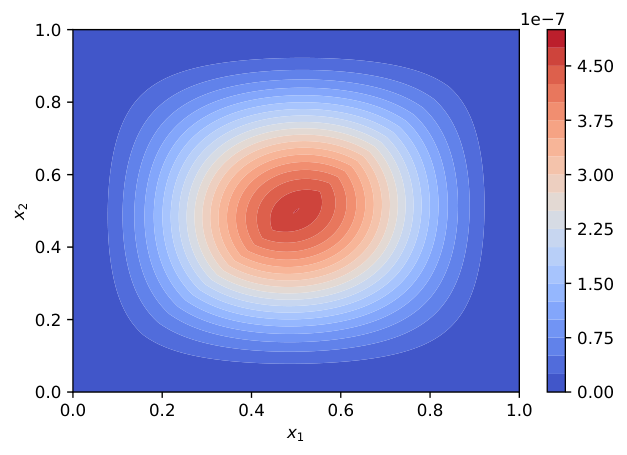
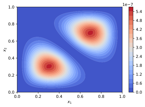
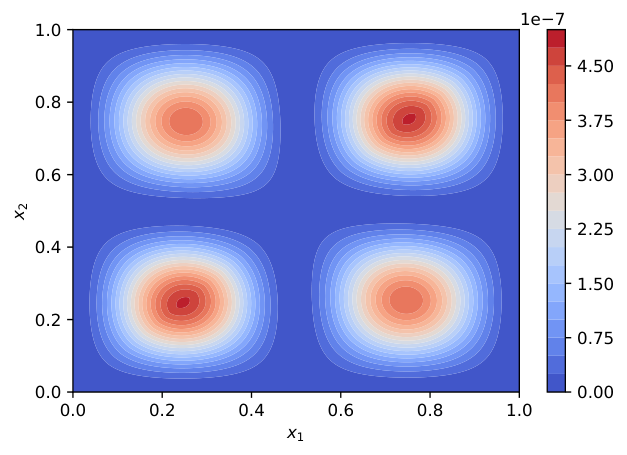
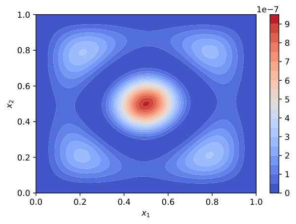
We plotted the complex momentum solutions for identical parity (i.e., when ) as a function of a negative interaction potential in Fig. 2. In particular, the complex solutions and are complex conjugates of one another, which ensures that the energy remains real. The imaginary components for the different parity, i.e., are essentially identical up to a sufficient level of numerical accuracy as illustrated in Fig. 2(b) and 2(d), although there are very slight differences in their values that are not discernable in the plots. These very minute differences arise from the weak dependence on in the radicand of Eq. (9) and (10), and the magnitude of their differences are more noticeable for . It was found that this perturbative treatment, combined with Newton’s method, does not yield correct momentum solutions for non-identical parity (i.e., when ). Consequently, the configuration interaction (CI) method was utilized to initially obtain a reliable approximation for the energy. This effectively reduces the degrees of freedom in our search, enabling Newton’s method to be implemented successfully (see the SM Sup). The momentum solutions for non-identical parity are purely real, whereas complex momentum solutions occur only for identical parity. The reason is that momentum solutions where cannot be complex conjugates of each other. The solutions must satisfy either Eq. (7) or Eq. (8), with the additional constraint of real energy given by , which can only be simultaneously fulfilled by real momentum solutions when parity . With the momentum solutions obtained, we can utilize Eq. (3) to plot the probability density for different states with a negative interaction potential of , as depicted in Fig. 3. The probability densities in Fig. 3(a) and 3(c) involve complex momentum solutions, whereas those in Fig. 3(b) and 3(d) are from real momentum solutions. We can compare the wavefunction under negative and positive interaction potentials by changing the value of from to and plotting the resulting probability density in Fig. 4. In Fig. 3(c), the probability density corresponding to the state is weaker along the diagonal and stronger along the diagonal. This is because, along the diagonal, the electrons are maximally separated from each other within the 1D quantum well. As a result, the attractive delta-function interaction plays no role. Conversely, along the diagonal, the two electrons are in the same position, and the negative interaction potential increases the probability of finding the electrons in this region. Fig. 4(b) displays a similar behavior but in reverse for a repulsive positive interaction potential where the probability density corresponding to the state is stronger along the diagonal and weaker along the diagonal.
 (a)
(a)
|
 (b)
(b)
|
 (c)
(c)
|
 (d)
(d)
|
 (a)
(a)
|
 (b)
(b)
|
IV Conclusions
In summary, we have demonstrated that two electrons forming a singlet state confined in a one-dimensional infinite quantum well, modeled by an effective attractive delta-function interaction potential between the two electrons, require complex momentum solutions in the case of identical parity. Perturbative analysis and Newton’s method allowed us to obtain these complex momentum solutions, which consisted of conjugate pairs. As a result, this provides evidence for the necessity of complex numbers within quantum theory while considering a simplified model. Although a more complicated model involving many-body effects from more than two electrons, a different attractive interaction potential, and higher dimensionality exists, our simplified model sufficiently highlights the importance of complex numbers in quantum mechanics. Furthermore, by incorporating the configuration interaction method, we also acquired real momentum solutions for non-identical parity. The probability densities for positive and negative interaction potentials appeared similar but differed most noticeably along the diagonals, i.e., when the two electrons had the same position, the negative(positive) interaction potential increased(decreased) the probability densities.
Acknowledgements.
Matthew Albert would like to acknowledge Daniel Miravet for the fruitful discussions on numerical implementations and for providing valuable resources. Liang Chen would like to acknowledge the discussion with Vladimir Kalosha.References
- Chen et al. (2022) M.-C. Chen, C. Wang, F.-M. Liu, J.-W. Wang, C. Ying, Z.-X. Shang, Y. Wu, M. Gong, H. Deng, F.-T. Liang, Q. Zhang, C.-Z. Peng, X. Zhu, A. Cabello, C.-Y. Lu, and J.-W. Pan, Physical review letters 128, 040403 (2022).
- Karam (2020) R. Karam, American journal of physics 88, 39 (2020).
- Miller (2022) J. L. Miller, Physics today 75, 14 (2022).
- Renou et al. (2021) M.-O. Renou, D. Trillo, M. Weilenmann, T. P. Le, A. Tavakoli, N. Gisin, A. Acín, and M. Navascués, Nature 600, 625 (2021).
- Li et al. (2022) Z.-D. Li, Y.-L. Mao, M. Weilenmann, A. Tavakoli, H. Chen, L. Feng, S.-J. Yang, M.-O. Renou, D. Trillo, T. P. Le, et al., Physical Review Letters 128, 040402 (2022).
- Aleksandrova et al. (2013) A. Aleksandrova, V. Borish, and W. K. Wootters, Physical Review A 87, 052106 (2013).
- Baez (2012) J. C. Baez, Foundations of Physics 42, 819 (2012).
- Myrheim (1999) J. Myrheim, arXiv preprint quant-ph/9905037 (1999).
- Bednorz and Batle (2022) A. Bednorz and J. Batle, Physical review. A 106 (2022).
- Birkhoff and Neumann (1936) G. Birkhoff and J. V. Neumann, Annals of Mathematics 37, 823 (1936).
- Stueckelberg (1960) E. C. Stueckelberg, Helv. Phys. Acta 33, 458 (1960).
- Guenin and Stueckelberg (1961) M. Guenin and E. Stueckelberg, Helv. Phys. Acta 34, 621 (1961).
- McKague et al. (2009) M. McKague, M. Mosca, and N. Gisin, Physical review letters 102, 020505 (2009).
- Ismael (2021) J. Ismael, in The Stanford Encyclopedia of Philosophy, edited by E. N. Zalta (Metaphysics Research Lab, Stanford University, 2021) Fall 2021 ed.
- Piron (1964) C. Piron, Helvetica physica acta 37, 439 (1964).
- ZUKOWSKI et al. (1993) M. ZUKOWSKI, A. ZEILINGER, M. A. HORNE, and A. K. EKERT, Physical review letters 71, 4287 (1993).
- Acín et al. (2015) A. Acín, S. Pironio, T. Vértesi, and P. Wittek, Physical review. A, Atomic, molecular, and optical physics 93 (2015).
- Bowles et al. (2018) J. Bowles, I. Šupić, D. Cavalcanti, and A. Acín, Physical review. A 98 (2018).
- Griffiths and Schroeter (2019) D. Griffiths and D. Schroeter, Introduction to Quantum Mechanics (Cambridge University Press, 2019).
- Franchini (2011) F. Franchini, International School for Advanced Studies-Trieste, Lecture Notes (2011).
- Karle (2021) A. Karle, Bethe ansatz for the one dimensional heisenberg model (2021), PHYS 502, Condensed Matter Physics.
- Bethe (1931) H. Bethe, Zeitschrift für Physik 71, 205 (1931).
- Busch et al. (1998) T. Busch, B.-G. Englert, K. Rzażewski, and M. Wilkens, Foundations of Physics 28, 549 (1998).
- Weber (1964) G. G. Weber, The Journal of chemical physics 40, 1762 (1964).
- (25) See Supplemental Material section for additional details.
- Sakurai and Napolitano (2017) J. Sakurai and J. Napolitano, Modern Quantum Mechanics (Cambridge University Press, 2017).
- Weisskopf (1981) V. F. Weisskopf, Contemporary physics 22, 375 (1981).
- Pogosov et al. (2010) W. V. Pogosov, M. Combescot, and M. Crouzeix, Physical Review B 81, 174514 (2010).
- Burden and Faires (2010) R. Burden and J. Faires, Numerical Analysis (Cengage Learning, 2010).
V Supplemental Material
V.1 Singlet Wavefunction
In this appendix, we will begin by deriving the expression for the singlet state as seen in Section II of the main text. First, consider a singlet spin state formed by the two electron spins. The Pauli exclusion principle demands that the spatial wave function be symmetric under the permutation operation Sakurai and Napolitano 2017. Formally we could write:
| (11) |
and written spatially as:
| (12) |
Projection to spatial wave function gives:
| (13) |
Which can be expanded as:
| (14) |
where defining and as normalization constants give Eq. (3) in the main text.
V.2 Perturbative Analysis
As stated in the main text, a comparison with the non-interacting case leads one to expect and solutions of Eq. (7) and (8) (in the main text) to lie in the neighborhood and where . We can let and then Eq. (7) becomes:
| (15) |
Consider a small deviation in and in that is assume Making this substitution along with Taylor approximating and keeping only terms up to third order in from the first of Eq. (15) gives:
| (16) |
Similarly for the second of Eq. (15) and using Eq. (16) gives:
| (17) |
Solving for gives:
| (18) |
which can be substituted into Eq. (16) for the case where yielding:
| (19) |
Using the quadratic formula on Eq. (19) allows us to obtain Eq. (9) and (10) in the main text. The same analysis can be done on Eq. (8) of the main text, and it will result in the same expressions for the case of .
V.3 Configuration Interaction Method
Defining and the Hamiltonian in Eq. (1) of the main text, in the region can be written as:
| (20) |
We can then scale the Hamiltonian by to obtain:
| (21) |
The normalized non-interacting single particle eigenstates are given by with energy and they satisfy the condition The normalized symmetric wavefunction is given by:
| (22) |
where . First we solve for the non-interacting elements of our Hamiltonian, this yields:
| (23) |
Similarly a longer expression for the interacting elements of the Hamiltonian can also be obtained:
| (24) |
We can construct our Hamiltonian matrix using Eq. (23) and (24), and then diagonalize this matrix to obtain the eigenenergies. Once we have the value of a particular energy corresponding to a specific eigenstate, we can use the relation (we have scaled the energies by ). We can express and as:
| (25) |
where and This choice ensures that the energy remains real, as Since we can rewrite Eq. (25):
| (26) |
The number of free parameters has reduced from three in Eq. (25) to two in Eq. (26), which allows for effective utilization of Newton’s method to solve for these momentum solutions.