Giant Emitters in a Structured Bath with Non-Hermitian Skin Effect
Abstract
Giant emitters derive their name from nonlocal field-emitter interactions and feature diverse self-interference effects. Most of the existing works on giant emitters have considered Hermitian waveguides or photonic lattices. In this work, we unveil how giant emitters behave if they are coupled to a non-Hermitian bath, i.e., a Hatano-Nelson (HN) model which features a non-Hermitian skin effect due to the asymmetric inter-site tunneling rates. We show that the behaviors of the giant emitters are closely related to the stability of the bath. In the convectively unstable regime, where the HN model can be mapped to a pseudo-Hermitian lattice, a giant emitter can either behave as in a Hermitian bath or undergo excitation amplification, depending on the relative strength of different emitter-bath coupling paths. Based on this mechanism, we can realize protected nonreciprocal interactions between giant emitters, with nonreciprocity opposite to that of the bath. Such giant-emitter effects are not allowed, however, if the HN model enters the absolutely unstable regime, where the coupled emitters always show secular energy growth. Our proposal provides a new paradigm of non-Hermitian quantum optics, which may be useful for, e.g., engineering effective interactions between quantum emitters and performing many-body simulations in the non-Hermitian framework.
Introduction.—Giant emitters, which feature (discrete) nonlocal interactions with a bath, are setting up a new quantum optical paradigm and attracting increasing interest Kockum 2021. A hallmark of giant emitters is that their effective relaxation rates and transition frequencies are closely related to the interference effects of the nonlocal couplings Kockum et al. 2014; Gustafsson et al. 2014; Guo et al. 2017; Andersson et al. 2019; Vadiraj et al. 2021. For example, consider a two-level giant emitter (with transition frequency ) that is coupled to a one-dimensional waveguide at two points and with identical coupling strength . Its effective relaxation rate (to the waveguide) is given by Kockum et al. 2014; Kannan et al. 2020
| (1) |
where and are the wave number and the density of states of the waveguide field at frequency , respectively. Clearly, the relaxation of the giant emitter is inhibited (enhanced) if is an odd (even) multiple of , which can be understood as the destructive (constructive) interference of the two coupling paths. Based on such interference effects, one can realize decoherence-free interaction (DFI) between giant emitters via the waveguide, provided that they are coupled to the waveguide in a “braided” structure with interleaved coupling points Kockum et al. 2018; Kannan et al. 2020; Carollo et al. 2020; Soro and Kockum 2022; Du et al. 2023a. This DFI is essentially different from DFIs arising from the overlaps of photon-atom bound states Bay et al. 1997; Lambropoulos et al. 2000; Shahmoon and Kurizki 2013, which require that the frequencies of the emitters fall within the band gap of the (structured) bath. Moreover, it is also possible to realize chiral spontaneous emission and bound states if an additional phase difference is encoded into the nonlocal emitter-bath interaction Wang et al. 2020; Wang and r. Li 2022; Du et al. 2022a; Chen et al. 2022; Du et al. 2023b; Joshi et al. 2023.
The above giant-emitter effects are based on (structured) waveguides governed by Bloch’s theorem Kittel 2005, which states that the wave functions of a translationally invariant Hermitian system are plane waves modulated by a spatially periodic phase factor. For the giant-emitter system above, this is manifested by the waveguide field acquiring a phase when traveling between coupling points. For clarity, hereafter we refer to the above effects as “conventional giant-emitter interference effects” (CGIEs). In contrast, non-Hermitian systems exhibit a plethora of peculiar properties with no Hermitian analogues Bender and Boettcher 1998; Bender 2007; Longhi 2009; Wu et al. 2014; Konotop et al. 2016; Feng et al. 2017a; El-Ganainy et al. 2018; Gong et al. 2018; Kawabata et al. 2019, such as exceptional points Heiss 2012; Minganti et al. 2019; Miri and Alù 2019; Bergholtz et al. 2021 and biorthogonal eigenstates Brody 2014; Kunst et al. 2018. In particular, the conventional Bloch theorem can break down in a class of non-Hermitian systems, which feature non-Hermitian skin effects and are governed by non-Bloch band theory Yokomizo and Murakami 2019; Yokomizo and Murakami 2020; Kawabata et al. 2020a; Xue et al. 2021; Yokomizo and Murakami 2023. The most typical example is the Hatano-Nelson (HN) model Hatano and Nelson 1996, a one-dimensional tight-binding lattice with asymmetric inter-site tunneling rates, whose experimental implementations include coupled-(ring)-resonator arrays with auxiliary couplers with engineered gain and loss Longhi et al. 2015a; Longhi et al. 2015b, cascaded quantum systems based on reservoir engineering Metelmann and Clerk 2015, discrete-time non-Hermitian quantum walks Weidemann et al. 2020; Weidemann et al. 2022; Liang et al. 2022, and photonic synthetic dimensions Song et al. 2020; Wang et al. 2021. The spectra of such non-Hermitian systems are quite sensitive to the boundary conditions, which can result in unconventional topological Bergholtz et al. 2021; Yao and Wang 2018; Yao et al. 2018; Okuma et al. 2020; Zhu et al. 2020; Budich and Bergholtz 2020; Kawabata et al. 2020b and quantum optical Longhi 2016; Roccati et al. 2022; Gong et al. 2023a; Gong et al. 2023b phenomena. In view of this, it is natural to ask how giant emitters behave in a bath with non-Hermitian skin effect.
To address this question, we here study the quantum dynamics of giant emitters coupled to an HN model. We reveal that the giant emitters can exhibit essentially different behaviors, depending on what regime of the HN model we consider and the relative strengths of the nonlocal couplings. In particular, we unveil a series of unconventional quantum optical phenomena, such as secular energy growth and protected nonreciprocal interatomic interactions with nonreciprocity opposite to the field, which have no counterparts in small-emitter nor Hermitian giant-emitter systems. These findings may find applications in quantum simulation and inspire further studies in non-Hermitian quantum optics.
Model.—We first consider a bosonic mode coupled to two lattice sites of an HN model [Fig. 1(a)]. In the interaction picture, the Hamiltonian is ( hereafter)
| (2) |
where is the annihilation operator of the th site of the HN model (we consider lattice sites in total; ); and are the nearest-neighbor tunneling amplitudes towards the left and right, respectively, with the base tunneling amplitude and describing the non-Hermiticity of the system ( becomes Hermitian when ); () is the coupling strength between mode and the th (th) site of the HN model. We have assumed that the emitter (i.e., mode ) is resonant with the lattice band center. Under open boundary conditions, the wave functions of the bare HN model can be written as with and () Lv et al. 2022. An imaginary gauge field Longhi et al. 2015b, described by the imaginary wave number , modifies the wave functions so that all of them pile up at one of the two lattice edges, depending on the relative strength of and . In other words, fields are amplified (attenuated) when traveling in the direction of the stronger (weaker) tunneling amplitude.
Before proceeding, we briefly motivate choosing a bosonic mode as a generalized giant emitter Wang et al. 2022. In the non-Hermitian case here, the dynamics do not conserve the norm of the initial state. For a single-excitation initial state, the total excitation number of the system at time can be larger than one, which in a photonic implementation of our model (e.g., a harmonic oscillator coupled to an unstable coupled-resonator array) can be understood as amplified optical intensity arising from the field amplification. In this case, it is more convenient to consider a bosonic mode since the dynamics of a two-level system could exhibit complicated nonlinear characteristics. Alternatively, the single-excitation assumption can be restored by, e.g., introducing uniform on-site losses to the lattice sites Roccati et al. 2022; Gong et al. 2023a; Gong et al. 2023b, as will be discussed below.
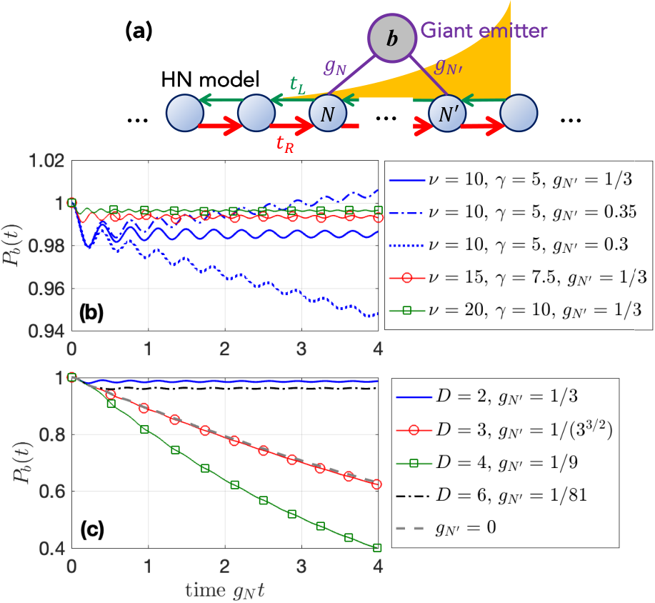
CGIEs in an HN model.—Now we show that, even in such a non-Bloch bath, it is possible to recover CGIEs by matching the relative coupling strength at the two coupling points with the non-Bloch phase factor . Figures 1(b) and 1(c) show the evolution of the mean particle number of the giant emitter , with system state ( is the ground state of the whole model) and initial condition Longhi 2016. To avoid boundary effects, we consider a long enough HN lattice with and . Moreover, we assume so that the non-Markovian retardation effect is weak Du et al. 2022a; Longhi 2020; Du et al. 2022b; Soro et al. 2023.
Figure 1(b) shows that the giant emitter exhibits a fractional decay [i.e., ] when and , although it is coupled to a non-Hermitian bath featuring directional field amplification and attenuation. This signifies the recovering of CGIEs in the sense that the emitter can be effectively decoupled from the bath due to the nonlocal interaction. The emitter tends to be completely dissipationless with the increase of the tunneling amplitudes, which is also consistent with the Hermitian case. Note that the fractional decay is sensitive to the relative strength : will increase (decrease) with time if is larger (smaller) than the critical value (cf. the blue dot-dashed and dotted lines). This effect means that the giant emitter can serve as a precise probe for the non-Hermiticity of the bath.
We also plot the evolution of for different values of in Fig. 1(c), with the matching condition always fulfilled. Again, similar to the Hermitian case, the giant emitter exhibits -dependent relaxation dynamics ranging from decoherence-free behavior (i.e., fractional decay for ) to superradiance-like behavior [i.e., enhanced relaxation for , compared to the small-atom case (gray dashed line)].
The recovered CGIEs can be understood from the self-energy of the giant emitter, which can be obtained (using the resolvent method Cohen-Tannoudji et al. 1998; see Sec. I of SM for details) as
| (3) |
with . The real and imaginary parts of represent the Lamb shift and effective relaxation rate, respectively, of due to its interaction with the bath. Under the Weisskopf-Wigner approximation Sakurai and Napolitano 2011 (valid for weak emitter-bath couplings), the dynamics of the emitter are well captured by the self-energy close to the real axis González-Tudela and Cirac 2017a; González-Tudela and Cirac 2017b, i.e., with the frequency detuning between the emitter and the band center. In the resonant case , with the matching condition , the self-energy simplifies to , which correctly predicts the dynamics in Fig. 1(b)-(c).
Nonreciprocal DFI.—One of the most important applications of CGIEs is in-band DFI between giant emitters Kannan et al. 2020; Kockum et al. 2018; Carollo et al. 2020; Soro and Kockum 2022; Du et al. 2023a. To explore whether this unique phenomenon is possible in the non-Bloch case, we extend the model in Eq. (2) to include an additional bosonic mode , with the coupling points of the two modes arranged in a braided structure. In the interaction picture, the Hamiltonian of this extended model is
| (4) |
where we assume that is coupled to sites and (with coupling strengths and , respectively) and is coupled to sites and (with coupling strengths and , respectively). Drawing on the result in Fig. 1, we set and so that and almost do not decay into the lattice.

Figures 2(a) and 2(b) depict the evolution of and , with system state , initial condition , and different values of . We find that and exchange energy in a nearly decoherence-free manner (there is a very weak decay due to the finite retardation effect) if the coupling strengths are matched as discussed above. In sharp contrast to the Hermitian case, the interaction here is nonreciprocal: the excitation is attenuated (amplified) when traveling from to (from to ). The attenuation/amplification is given by , as shown by the gray dashed lines in Fig. 2, which is determined by the non-Bloch phase factor as well as the coupling separation of each giant emitter.
This phenomenon can be understood from the interaction parts of the self-energy of the emitters, which are obtained (see Sec. II of SM for details) as
| (5) |
Since the real and imaginary parts of represent the effective coherent interaction from to ( to ) and the collective relaxation of the two emitters, respectively, it is clear that and interact with each other in a decoherence-free but nonreciprocal manner, with a strength ratio for the two directions. Most interestingly, the nonreciprocity of the interaction is opposite to that of the bath: while the HN model amplifies right-moving fields, the emitter pair has a stronger interaction towards the left ( is placed to the right of ). As we show in Sec. III of SM, this reversed nonreciprocity can be understood in an intuitive picture based on hidden bound states Gong et al. 2023a; Gong et al. 2023b induced by the interaction between the emitters and the HN model.
Absolutely unstable regime—So far, we have focused on the “convectively unstable regime” with Longhi 2016, where the HN model can be mapped to a pseudo-Hermitian lattice subject to an imaginary gauge field (see Sec. I of SM). In fact, there is a transition point (in this work, we always assume ) beyond which the HN model enters the “absolutely unstable regime” (where ). In the convectively unstable regime, a small emitter displays a complete (fractional) decay if its frequency is inside (outside) the energy band of the lattice. In the absolutely unstable regime, however, a small emitter has a secular pseudo-exponential energy growth Longhi 2016. This phenomenon can be interpreted as a competition between the amplification and the effective transport of the field in the HN model (see Sec. IV of SM): in the absolutely unstable regime, there is always a residual excitation component at the coupling point, suffering rapid amplification before being transferred away.

In contrast to the small-emitter case, a giant emitter can exhibit a secular growth even in the convectively unstable regime [see Fig. 1(b)]. This is due to the reabsorption of excitations emitted from another coupling point at an earlier moment and amplified by traveling in the HN model. This amplification mechanism, which arises from the combination of the giant-atom interference effect and the non-Hermiticity, is essentially different from that of a small emitter in the absolutely unstable regime.
We find that the CGIEs in Fig. 1 cannot be realized in the absolutely unstable regime. Instead, a giant emitter behaves somewhat like a small one in the sense of the secular amplification. As shown in Fig. 3, the giant emitter always shows a pseudo-exponential energy growth; the growth rate increases monotonically with the coupling strength ( is fixed). This is a bit different from the small-emitter case, where the emitter decays considerably before the secular growth.
Giant and small emitters also exhibit very different behaviors at the transition point . As shown in Fig. 3(c), a small emitter simply exchanges energy with the coupled site since their dynamics is decoupled from the rest of the system Longhi 2016, whereas a giant emitter shows energy growth since diverges at this point and the coupling matching condition thus cannot be fulfilled.
Giant emitter coupled to a stable HN model.—A standard HN model is unstable (convectively or absolutely). Its spectrum forms a loop in the complex plane, with the imaginary part positive for some values of [see the blue solid loop in Fig. 4(a)]. However, here we demonstrate how a giant emitter behaves if it is coupled to a stable HN model with large enough on-site losses Gong et al. 2023a; Gong et al. 2023b.

To this end, we assume in Eq. (2) with describing uniform on-site losses of the lattice. As shown in Fig. 4(a), the spectrum of the HN model is within the lower half-plane in this case (green dotted loop). This implies that the whole system becomes stable, without field amplification in the lattice.
Figure 4(b) shows the time evolution of for different values of . Similar to the Hermitian case Longhi 2020; Zhao and Wang 2020; Soro et al. 2023, the relaxation dynamics of the emitter depend on the coupling separation (i.e., on the phase accumulation of emitted photons traveling between coupling points) with no need to match the nonlocal couplings. However, fractional decay of the giant emitter is unavailable in this case, regardless of the value of , as shown in Fig. 4(c). This can be understood from the bath now becoming purely dissipative so that the field always is attenuated when traveling between the coupling points. Thus, in a stable HN model, the giant emitter behaves as in a Bloch structured bath with uniform on-site losses. Moreover, Fig. 4(d) shows that, in the stable regime, the giant emitter no longer exhibits qualitatively different dynamics for different signs of , i.e., the transition point of the HN model disappears in this regime.
Conclusion and outlook.—We have unveiled the self-interference effects of giant emitters coupled to an HN model, i.e., a structured bath featuring a non-Hermitian skin effect. The behaviors of giant emitters in this setting depend on the stability of the bath, which is closely related to the tunneling asymmetry. In the convectively unstable regime, where the HN model is equivalent to a pseudo-Hermitian lattice, CGIEs can be recovered by matching the nonlocal emitter-bath coupling strengths. In particular, we identify a non-Hermitian DFI condition under which the giant emitters show protected but nonreciprocal interactions. If the HN model enters the absolutely unstable regime, giant emitters exhibit secular energy growth just like the small emitters. An HN model made stable by introducing uniform on-site losses simply behaves like a Bloch (but dissipative) structured bath in the sense that giant emitters always show CGIEs with no need to match the nonlocal couplings.
Our findings can inspire a number of further investigations. For example, it has been shown recently that the HN model can be mapped to a two-dimensional hyperbolic lattice with the effective curvature determined by the non-Hermiticity Lv et al. 2022; Wang and Wan 2022. It thus provides an exciting opportunity to explore giant-emitter physics in curved spaces without judiciously distorting the spatial configuration of a kagome lattice Kollár et al. 2019; Bienias et al. 2022. In Sec. V of SM, we provide a brief discussion of designing a giant emitter coupled to such an effective hyperbolic lattice. Moreover, it is known that the spectra of some non-Hermitian topological insulators are sensitive to the boundary condition such that the conventional bulk-boundary correspondence no longer can predict the existence of their edge states Gong et al. 2018; Bergholtz et al. 2021; Yao and Wang 2018; Yao et al. 2018; Okuma et al. 2020; Zhu et al. 2020. Studying how giant emitters affect these systems can be interesting since it shows the possibility of probing the topological phase and creating unconventional, topologically protected bound states. Considering the exotic behaviors of giant emitters in (Hermitian) two-dimensional lattices González-Tudela et al. 2019; Vega et al. 2023; Ingelsten et al., it could also be interesting to introduce the non-Hermitian skin effect to higher-dimensional baths Kawabata et al. 2020b; Song et al. 2020 and study their interplay with giant emitters. The results, such as the nonreciprocal DFIs, hold promise for non-Hermitian many-body simulations due to the interaction protection mechanism in a non-Hermitian bath Feng et al. 2017b.
Acknowledgements.
Acknowledgments.—LD thanks Francesco Ciccarello and Xin Wang for helpful discussions. YZ is supported by the National Natural Science Foundation of China (under Grant No. 12074061). AFK acknowledges support from the Swedish Research Council (grant number 2019-03696), from the Swedish Foundation for Strategic Research, and from the Knut and Alice Wallenberg Foundation through the Wallenberg Centre for Quantum Technology (WACQT).References
- Kockum (2021) A. F. Kockum, Quantum Optics with Giant Atoms—the First Five Years, in International Symposium on Mathematics, Quantum Theory, and Cryptography, edited by T. Takagi, M. Wakayama, K. Tanaka, N. Kunihiro, K. Kimoto, and Y. Ikematsu (Springer Singapore, Singapore, 2021) pp. 125–146.
- Kockum et al. (2014) A. F. Kockum, P. Delsing, and G. Johansson, Designing frequency-dependent relaxation rates and Lamb shifts for a giant artificial atom, Phys. Rev. A 90, 013837 (2014).
- Gustafsson et al. (2014) M. V. Gustafsson, T. Aref, A. F. Kockum, M. K. Ekström, G. Johansson, and P. Delsing, Propagating phonons coupled to an artificial atom, Science 346, 207 (2014).
- Guo et al. (2017) L. Guo, A. Grimsmo, A. F. Kockum, M. Pletyukhov, and G. Johansson, Giant acoustic atom: A single quantum system with a deterministic time delay, Phys. Rev. A 95, 053821 (2017).
- Andersson et al. (2019) G. Andersson, B. Suri, L. Guo, T. Aref, and P. Delsing, Non-exponential decay of a giant artificial atom, Nat. Phys. 15, 1123 (2019).
- Vadiraj et al. (2021) A. M. Vadiraj, A. Ask, T. G. McConkey, I. Nsanzineza, C. W. Sandbo Chang, A. F. Kockum, and C. M. Wilson, Engineering the level structure of a giant artificial atom in waveguide quantum electrodynamics, Phys. Rev. A 103, 023710 (2021).
- Kannan et al. (2020) B. Kannan, M. Ruckriegel, D. Campbell, A. F. Kockum, J. Braumüller, D. Kim, M. Kjaergaard, P. Krantz, A. Melville, B. M. Niedzielski, A. Vepsäläinen, R. Winik, J. Yoder, F. Nori, T. P. Orlando, S. Gustavsson, and W. D. Oliver, Waveguide quantum electrodynamics with superconducting artificial giant atoms, Nature (London) 583, 775 (2020).
- Kockum et al. (2018) A. F. Kockum, G. Johansson, and F. Nori, Decoherence-Free Interaction between Giant Atoms in Waveguide Quantum Electrodynamics, Phys. Rev. Lett. 120, 140404 (2018).
- Carollo et al. (2020) A. Carollo, D. Cilluffo, and F. Ciccarello, Mechanism of decoherence-free coupling between giant atoms, Phys. Rev. Res. 2, 043184 (2020).
- Soro and Kockum (2022) A. Soro and A. F. Kockum, Chiral quantum optics with giant atoms, Phys. Rev. A 105, 023712 (2022).
- Du et al. (2023a) L. Du, L. Guo, and Y. Li, Complex decoherence-free interactions between giant atoms, Phys. Rev. A 107, 023705 (2023a).
- Bay et al. (1997) S. Bay, P. Lambropoulos, and K. Mölmer, Atom-atom interaction in strongly modified reservoirs, Phys. Rev. A 55, 1485 (1997).
- Lambropoulos et al. (2000) P. Lambropoulos, G. M. Nikolopoulos, T. R. Nielsen, and S. Bay, Fundamental quantum optics in structured reservoirs, Rep. Prog. Phys. 63, 455 (2000).
- Shahmoon and Kurizki (2013) E. Shahmoon and G. Kurizki, Nonradiative interaction and entanglement between distant atoms, Phys. Rev. A 87, 033831 (2013).
- Wang et al. (2020) X. Wang, T. Liu, A. F. Kockum, H.-R. Li, and F. Nori, Tunable Chiral Bound States with Giant Atoms, Phys. Rev. Lett. 126, 043602 (2020).
- Wang and r. Li (2022) X. Wang and H. r. Li, Chiral quantum network with giant atoms, Quantum Sci. Technol. 7, 035007 (2022).
- Du et al. (2022a) L. Du, Y. Zhang, J.-H. Wu, A. F. Kockum, and Y. Li, Giant Atoms in a Synthetic Frequency Dimension, Phys. Rev. Lett. 128, 223602 (2022a).
- Chen et al. (2022) Y.-T. Chen, L. Du, L. Guo, Z. Wang, Y. Zhang, Y. Li, and J.-H. Wu, Nonreciprocal and chiral single-photon scattering for giant atoms, Commun. Physc. 5, 215 (2022).
- Du et al. (2023b) L. Du, Y.-T. Chen, Y. Zhang, Y. Li, and J.-H. Wu, Decay dynamics of a giant atom in a structured bath with broken time-reversal symmetry, Quantum Sci. Technol. 8, 045010 (2023b).
- Joshi et al. (2023) C. Joshi, F. Yang, and M. Mirhosseini, Resonance Fluorescence of a Chiral Artificial Atom, Phys. Rev. X 13, 021039 (2023).
- Kittel (2005) C. Kittel, Introduction to Solid State Physics (Weily, New York, 2005).
- Bender and Boettcher (1998) C. M. Bender and S. Boettcher, Real Spectra in Non-Hermitian Hamiltonians Having Symmetry, Phys. Rev. Lett. 80, 5243 (1998).
- Bender (2007) C. M. Bender, Making sense of non-Hermitian Hamiltonians, Rep. Prog. Phys. 70, 947 (2007).
- Longhi (2009) S. Longhi, Bloch Oscillations in Complex Crystals with Symmetry, Phys. Rev. Lett. 103, 123601 (2009).
- Wu et al. (2014) J.-H. Wu, M. Artoni, and G. C. La Rocca, Non-Hermitian Degeneracies and Unidirectional Reflectionless Atomic Lattices, Phys. Rev. Lett. 113, 123004 (2014).
- Konotop et al. (2016) V. V. Konotop, J. Yang, and D. A. Zezyulin, Nonlinear waves in -symmetric systems, Rev. Mod. Phys. 88, 035002 (2016).
- Feng et al. (2017a) L. Feng, R. El-Ganainy, and L. Ge, Non-hermitian photonics based on parity-time symmetry, Nat. Photon. 11, 752 (2017a).
- El-Ganainy et al. (2018) R. El-Ganainy, K. G. Makris, M. Khajavikhan, Z. H. Musslimani, S. Rotter, and D. N. Christodoulides, Non-hermitian physics and PT symmetry, Nat. Phys. 14, 11 (2018).
- Gong et al. (2018) Z. Gong, Y. Ashida, K. Kawabata, K. Takasan, S. Higashikawa, and M. Ueda, Topological Phases of Non-Hermitian Systems, Phys. Rev. X 8, 031079 (2018).
- Kawabata et al. (2019) K. Kawabata, K. Shiozaki, M. Ueda, and M. Sato, Symmetry and Topology in Non-Hermitian Physics, Phys. Rev. X 9, 041015 (2019).
- Heiss (2012) W. D. Heiss, The physics of exceptional points, J. Phys. A 45, 444016 (2012).
- Minganti et al. (2019) F. Minganti, A. Miranowicz, R. W. Chhajlany, and F. Nori, Quantum exceptional points of non-Hermitian Hamiltonians and Liouvillians: The effects of quantum jumps, Phys. Rev. A 100, 062131 (2019).
- Miri and Alù (2019) M.-A. Miri and A. Alù, Exceptional points in optics and photonics, Science 363, eaar7709 (2019).
- Bergholtz et al. (2021) E. J. Bergholtz, J. C. Budich, and F. K. Kunst, Exceptional topology of non-Hermitian systems, Rev. Mod. Phys. 93, 015005 (2021).
- Brody (2014) D. C. Brody, Biorthogonal quantum mechanics, J. Phys. A 47, 035305 (2014).
- Kunst et al. (2018) F. K. Kunst, E. Edvardsson, J. C. Budich, and E. J. Bergholtz, Biorthogonal Bulk-Boundary Correspondence in Non-Hermitian Systems, Phys. Rev. Lett. 121, 026808 (2018).
- Yokomizo and Murakami (2019) K. Yokomizo and S. Murakami, Non-Bloch Band Theory of Non-Hermitian Systems, Phys. Rev. Lett. 123, 066404 (2019).
- Yokomizo and Murakami (2020) K. Yokomizo and S. Murakami, Non-Bloch band theory and bulk–edge correspondence in non-Hermitian systems, Prog. Theor. Exp. Phys. 2020, 12A102 (2020).
- Kawabata et al. (2020a) K. Kawabata, N. Okuma, and M. Sato, Non-Bloch band theory of non-Hermitian Hamiltonians in the symplectic class, Phys. Rev. B 101, 195147 (2020a).
- Xue et al. (2021) W.-T. Xue, M.-R. Li, Y.-M. Hu, F. Song, and Z. Wang, Simple formulas of directional amplification from non-Bloch band theory, Phys. Rev. B 103, L241408 (2021).
- Yokomizo and Murakami (2023) K. Yokomizo and S. Murakami, Non-Bloch bands in two-dimensional non-Hermitian systems, Phys. Rev. B 107, 195112 (2023).
- Hatano and Nelson (1996) N. Hatano and D. R. Nelson, Localization Transitions in Non-Hermitian Quantum Mechanics, Phys. Rev. Lett. 77, 570 (1996).
- Longhi et al. (2015a) S. Longhi, D. Gatti, and G. D. Valle, Robust light transport in non-Hermitian photonic lattices, Sci. Rep. 5, 13376 (2015a).
- Longhi et al. (2015b) S. Longhi, D. Gatti, and G. D. Valle, Non-Hermitian transparency and one-way transport in low-dimensional lattices by an imaginary gauge field, Phys. Rev. B 92, 094204 (2015b).
- Metelmann and Clerk (2015) A. Metelmann and A. A. Clerk, Nonreciprocal Photon Transmission and Amplification via Reservoir Engineering, Phys. Rev. X 5, 021025 (2015).
- Weidemann et al. (2020) S. Weidemann, M. Kremer, T. Helbig, T. Hofmann, A. Stegmaier, M. Greiter, R. Thomale, and A. Szameit, Topological funneling of light, Science 368, 311 (2020).
- Weidemann et al. (2022) S. Weidemann, M. Kremer, S. Longhi, and A. Szameit, Topological triple phase transition in non-Hermitian Floquet quasicrystals, Nature (London) 601, 354 (2022).
- Liang et al. (2022) Q. Liang, D. Xie, Z. Dong, H. Li, H. Li, B. Gadway, W. Yi, and B. Yan, Dynamic Signatures of Non-Hermitian Skin Effect and Topology in Ultracold Atoms, Phys. Rev. Lett. 129, 070401 (2022).
- Song et al. (2020) Y. Song, W. Liu, L. Zheng, Y. Zhang, B. Wang, and P. Lu, Two-dimensional non-Hermitian Skin Effect in a Synthetic Photonic Lattice, Phys. Rev. Appl. 14, 064076 (2020).
- Wang et al. (2021) K. Wang, A. Dutt, K. Y. Yang, C. C. Wojcik, J. Vučković, and S. Fan, Generating arbitrary topological windings of a non-Hermitian band, Science 371, 1240 (2021).
- Yao and Wang (2018) S. Yao and Z. Wang, Edge States and Topological Invariants of Non-Hermitian Systems, Phys. Rev. Lett. 121, 086803 (2018).
- Yao et al. (2018) S. Yao, F. Song, and Z. Wang, Non-Hermitian Chern Bands, Phys. Rev. Lett. 121, 136802 (2018).
- Okuma et al. (2020) N. Okuma, K. Kawabata, K. Shiozaki, and M. Sato, Topological Origin of Non-Hermitian Skin Effects, Phys. Rev. Lett. 124, 086801 (2020).
- Zhu et al. (2020) X. Zhu, H. Wang, S. K. Gupta, H. Zhang, B. Xie, M. Lu, and Y. Chen, Photonic non-Hermitian skin effect and non-Bloch bulk-boundary correspondence, Phys. Rev. Res. 2, 013280 (2020).
- Budich and Bergholtz (2020) J. C. Budich and E. J. Bergholtz, Non-Hermitian Topological Sensors, Phys. Rev. Lett. 125, 180403 (2020).
- Kawabata et al. (2020b) K. Kawabata, M. Sato, and K. Shiozaki, Higher-order non-Hermitian skin effect, Phys. Rev. B 102, 205118 (2020b).
- Longhi (2016) S. Longhi, Quantum decay and amplification in a non-Hermitian unstable continuum, Phys. Rev. A 93, 062129 (2016).
- Roccati et al. (2022) F. Roccati, S. Lorenzo, G. Calajò, G. M. Palma, A. Carollo, and F. Ciccarello, Exotic interactions mediated by a non-Hermitian photonic bath, Optica 9, 565 (2022).
- Gong et al. (2023a) Z. Gong, M. Bello, D. Malz, and F. K. Kunst, Anomalous Behaviors of Quantum Emitters in Non-Hermitian Baths, Phys. Rev. Lett. 129, 223601 (2023a).
- Gong et al. (2023b) Z. Gong, M. Bello, D. Malz, and F. K. Kunst, Bound states and photon emission in non-Hermitian nanophotonics, Phys. Rev. A 106, 053517 (2023b).
- Lv et al. (2022) C. Lv, R. Zhang, Z. Zhai, and Q. Zhou, Curving the space by non-hermiticity, Nat. Commun. 13, 2184 (2022).
- Wang et al. (2022) Z.-Q. Wang, Y.-P. Wang, J. Yao, R.-C. Shen, W.-J. Wu, J. Qian, J. Li, S.-Y. Zhu, and J. Q. You, Giant spin ensembles in waveguide magnonics, Nat. Commun. 13, 7580 (2022).
- Longhi (2020) S. Longhi, Photonic simulation of giant atom decay, Opt. Lett. 45, 3017 (2020).
- Du et al. (2022b) L. Du, Y.-T. Chen, Y. Zhang, and Y. Li, Giant atoms with time-dependent couplings, Phys. Rev. Res. 4, 023198 (2022b).
- Soro et al. (2023) A. Soro, C. S. Muñoz, and A. F. Kockum, Interaction between giant atoms in a one-dimensional structured environment, Phys. Rev. A 107, 013710 (2023).
- Cohen-Tannoudji et al. (1998) C. Cohen-Tannoudji, J. Dupont-Roc, and G. Grynberg, Nonperturbative Calculation of Transition Amplitudes, in Atom—Photon Interactions (John Wiley & Sons, Ltd, 1998) Chap. 3, pp. 165–255.
- (67) See Supplemental Material at http://xxxxxx for more details .
- Sakurai and Napolitano (2011) J. J. Sakurai and J. Napolitano, Modern Quantum Mechanics (Addison-Wesley, Boston, 2011).
- González-Tudela and Cirac (2017a) A. González-Tudela and J. I. Cirac, Quantum Emitters in Two-Dimensional Structured Reservoirs in the Nonperturbative Regime, Phys. Rev. Lett. 119, 143602 (2017a).
- González-Tudela and Cirac (2017b) A. González-Tudela and J. I. Cirac, Markovian and non-Markovian dynamics of quantum emitters coupled to two-dimensional structured reservoirs, Phys. Rev. A 96, 043811 (2017b).
- Zhao and Wang (2020) W. Zhao and Z. Wang, Single-photon scattering and bound states in an atom-waveguide system with two or multiple coupling points, Phys. Rev. A 101, 053855 (2020).
- Wang and Wan (2022) S.-X. Wang and S. Wan, Duality between the generalized non-Hermitian Hatano-Nelson model in flat space and a Hermitian system in curved space, Phys. Rev. B 106, 075112 (2022).
- Kollár et al. (2019) A. J. Kollár, M. Fitzpatrick, and A. A. Houck, Hyperbolic lattices in circuit quantum electrodynamics, Nature (London) 571, 45 (2019).
- Bienias et al. (2022) P. Bienias, I. Boettcher, R. Belyansky, A. J. Kollár, and A. V. Gorshkov, Circuit Quantum Electrodynamics in Hyperbolic Space: From Photon Bound States to Frustrated Spin Models, Phys. Rev. Lett. 128, 013601 (2022).
- González-Tudela et al. (2019) A. González-Tudela, C. S. Muñoz, and J. I. Cirac, Engineering and Harnessing Giant Atoms in High-Dimensional Baths: A Proposal for Implementation with Cold Atoms, Phys. Rev. Lett. 122, 203603 (2019).
- Vega et al. (2023) C. Vega, D. Porras, and A. González-Tudela, Topological multimode waveguide QED, Phys. Rev. Res. 5, 023031 (2023).
- (77) E. Ingelsten, A. F. Kockum, and A. Soro, Giant atoms in a two-dimensional structured environment, in preparation .
- Feng et al. (2017b) L. Feng, R. El-Ganainy, and L. Ge, Non-Hermitian photonics based on parity–time symmetry, Nat. Photon. 11, 752 (2017b).
- Bekenstein et al. (2017) R. Bekenstein, Y. Kabessa, Y. Sharabi, O. Tal, N. Engheta, G. Eisenstein, A. J. Agranat, and M. Segev, Control of light by curved space in nanophotonic structures, Nat. Photon. 11, 664 (2017).
- Schine et al. (2019) N. Schine, M. Chalupnik, T. Can, A. Gromov, and J. Simon, Electromagnetic and gravitational responses of photonic Landau levels, Nature (London) 565, 173 (2019).
- Zhang et al. (2021) R. Zhang, C. Lv, Y. Yan, and Q. Zhou, Efimov-like states and quantum funneling effects on synthetic hyperbolic surfaces, Sci. Bull. 66, 1967 (2021).
Supplemental Material for “Giant Emitters in a Structured Bath with Non-Hermitian Skin Effect”
Lei Du1,2, Lingzhen Guo3, Yan Zhang1, and Anton Frisk Kockum2
1 Center for Quantum Sciences and School of Physics,
Northeast Normal University, Changchun 130024, China
2 Department of Microtechnology and Nanoscience,
Chalmers University of Technology, 412 96 Gothenburg, Sweden
3 Center for Joint Quantum Studies and Department of Physics, School of Science,
Tianjin University, Tianjin 300072, China
I I. Self-energy of a giant emitter coupled to a Hatano-Nelson model
The dynamics of the single giant emitter can be clearly illustrated using the resolvent method Cohen-Tannoudji et al. 1998. The resolvent of the whole system (i.e., emitterbath) is
| (S1) |
where is the free Hamiltonian of the emitter and the bare Hatano-Nelson (HN) model and describes the emitter-lattice interaction. For a projector of the eigenstates of and its complementary , the resolvent satisfies
| (S2) |
where
| (S3) |
is the so-called level-shift operator. Note that the second-order perturbation expansion in Eq. (S3) is justified if is small compared to . By using the projector (projecting onto the state of emitter ) and its complementary (projecting onto the states of the bath), the self-energy of can be given by .
If both and are positive (i.e., the HN model is in the convectively unstable regime Longhi 2016), the Hamiltonian of the HN model can be rewritten as Longhi et al. 2015b
| (S4) |
Its eigenvalues are given by
| (S5) |
where is a complex wave number and is the resonance frequency of each lattice site as well as emitter (we assume that the emitter is resonant with the lattice band center). This implies that the HN model can be viewed as a one-dimensional pseudo-Hermitian lattice subject to an imaginary gauge field. In view of this, by performing the transformation
| (S6) |
the Hamiltonian in Eq. (2) in the main text can be rewritten as
| (S7) | |||||
| (S8) | |||||
| (S9) |
with , , , and . Here is the -space annihilation operator of the lattice field, satisfying and . It is worth noting that is real and in general not a function of .
Substituting Eqs. (S8) and (S9) into Eq. (S3), the self-energy of is obtained as
| (S10) |
where in the last step we have changed the integral variable as and replaced by (only even functions contribute to the integral). By setting such that and , we have
| (S11) |
By using the residue theorem, we finally arrive at
| (S12) |
with . In the case of weak emitter-bath couplings (i.e., under the Weisskopf-Wigner approximation), the dynamics of the emitter are well captured by the self-energy close to the real axis González-Tudela and Cirac 2017a; González-Tudela and Cirac 2017b, i.e., with the frequency detuning between the emitter and the middle of the energy band. If is exactly resonant with the band center (i.e., ), one has and Eq. (S12) can be simplified to
| (S13) |
Clearly, Eq. (S13) can correctly predict the dynamics in Fig. 1 in the main text if .
II II. Nonreciprocal decoherence-free interaction in the braided double-giant-emitter model
In this section, we aim to calculate the effective interaction between the two braided giant emitters and considered in the main text. By using the transformation in Eq. (S6), the Hamiltonian in Eq. (4) in the main text becomes , where is given in Eq. (S8) and
| (S14) |
with (). Note that in Eq. (S14) the last two terms are not the Hermitian conjugates of the first two ones since is complex.
Once again, by substituting Eqs. (S8) and (S14) into Eq. (S1), the resolvent of the two-giant-emitters model can be transformed by the projector (projecting onto the states of the emitters and ) into a matrix form, i.e.,
| (S15) |
where , (), and . If and as assumed in the main text, the self-energy of can be obtained as
| (S16) |
which is identical with that of the single-emitter case [cf. Eq. (S12) for and ]. Since the emitters and are identical, one can readily verify that . Clearly, the individual relaxations of and , which are described by the imaginary parts of and , are inhibited if both and are resonant with the band center of the HN model.
Moreover, the interaction parts and , i.e., the off-diagonal elements of Eq. (S15), can be obtained as
| (S17) |
and
| (S18) |
When and are resonant with the band center of the HN model and under the Weisskopf-Wigner approximation, we have
| (S19) | |||||
| (S20) |
which are purely real (keeping in mind that has been assumed). Since the real and imaginary parts of describe the effective coherent coupling from to (from to ) and the collective relaxation of the two emitters, respectively, we conclude from Eqs. (S19) and (S20) that there is a nonreciprocal decoherence-free interaction (with a weight difference ) between and .
With a similar procedure, we can also calculate the interaction parts and in a more general case with arbitrary coupling separations [beyond the nearest-neighbor coupling points in Eq. (S14)]. For example, we can immediately obtain
| (S21) | |||||
| (S22) |
where is the separation between the left coupling points of the two giant emitters [ in Eqs. (S19) and (S20)] and is the separation between the two coupling points of each giant emitter [ in Eqs. (S19) and (S20)]. For simplicity, we have assumed identical separation for both emitters. It is clear from Eqs. (S21) and (S22) that if , there is always a nonreciprocal decoherence-free interaction which is manifested by the strength difference . However, the coupling strengths decay with the increase of and and the decay rate is determined by the non-Hermiticity (i.e., the value of ).
III III. Hidden bound states
It has been shown that there are two essentially different bound states that can arise when considering a small emitter coupled to an HN model Gong et al. 2023a. If the frequency of the emitter falls within the energy band of the HN model (within the energy loop in the complex plane), there is always a hidden bound state localized around the emitter-lattice coupling point, whose energy is exactly pinned at the frequency of the emitter. This bound state shows a chiral photonic profile which decays exponentially in the direction of the weaker tunneling rate, as shown in Fig. S1(a). On the other hand, conventional bound states can be formed if the frequency of the emitter falls outside the energy band. In contrast to the Hermitian case, the conventional bound states here appear only if the emitter-lattice coupling strength is large enough. If several small emitters (which can have different frequencies) are coupled to a common HN model, the photonic profile of the hidden bound state is a superposition of those arising from each atom, as if the emitters do not influence each other Gong et al. 2023b.
In this section, we briefly discuss the hidden bound states induced by a giant emitter coupled to an HN model. For a single giant emitter, as shown in Fig. S1(b), the photonic profile of the resulting hidden bound state is also a superposition of those arising from each coupling point. However, the components induced by the two coupling points are quite imbalanced due to the unequal coupling strengths. With the matching condition fulfilled, the component induced by the right coupling point diminishes rapidly as the coupling separation increases, as shown in Fig. S1(c).
In fact, the hidden bound states can provide an intuitive but qualitative picture to understand the nonreciprocal decoherence-free interaction in Fig. 2 in the main text (whose nonreciprocity is opposite to that of the HN model). As discussed above, each giant emitter can produce a hidden bound state with a highly chiral photonic profile with respect to its two coupling points. If an emitter is located in the range of the bound state induced by another emitter , the intensity of the bound state at the coupling point of determines the effective coupling strength from to through this coupling path. In the case of Fig. 2 in the main text, the intensities of the hidden bound state (i.e., induced by ) at the coupling points of are smaller than the intensities of the hidden bound state (i.e., induced by ) at the coupling points of , as shown in Fig. S1(d). Keeping in mind that this is almost the only path that mediates the interaction between the two emitters (both of them nearly do not decay into the lattice), they thus exhibit nonreciprocal interaction with opposite direction preference with respect to the HN model.
IV IV. Dynamics of a small emitter in the convectively and absolutely unstable regimes

As discussed in Sec. I, an HN model is equivalent to a pseudo-Hermitian lattice subject to an imaginary gauge field when (i.e., in the convectively unstable regime). The imaginary gauge field, which is manifested by the complex wave number , can be eliminated by performing the transformation
| (S23) |
In this regime, the relaxation dynamics of a small emitter resembles the Hermitian case. As shown in Fig. S2(a), although the field is amplified when traveling along the direction of the larger tunneling rate, it can be transferred away rapidly with almost no remnant at each passing lattice site in the long-time limit [i.e., for any given lattice site , its field intensity for ]. This implies that the instability is transient in this case Longhi 2016. Therefore, the emitter shows an irreversible complete decay if its transition frequency lies within the energy band of the HN model, as shown in Fig. S2(b).
In the absolutely unstable regime (i.e., and ), however, the HN model cannot be mapped to a pseudo-Hermitian one. In this case, the decay-dynamics problem becomes purely non-Hermitian. As shown in Fig. S2(c), the excitation is strongly amplified after entering the HN model, similar to the convectively unstable case. However, at the coupled site there is always a considerable remnant suffering permanent amplification [i.e., for ]. In other words, the local amplification effect surpasses the effective transport capability of the HN model so that the emitter shows a secular energy growth, as shown in Fig. S2(d).
V V. Mapping to curved spaces

Very recently, it has been shown that a class of non-Hermitian systems can simulate quantum systems in curved spaces Lv et al. 2022; Wang and Wan 2022. In particular, an HN model can be mapped to a two-dimensional hyperbolic lattice whose curvature is determined by the non-Hermiticity . While conventional schemes of implementing hyperbolic lattices require that the spatial structure of a physical system has to be distorted to become curved Kollár et al. 2019; Bienias et al. 2022; Bekenstein et al. 2017; Schine et al. 2019, this duality (between the non-Hermitian systems and their hyperbolic counterparts) allows for simulating hyperbolic spaces using lattices with fixed lattice constants. For the HN model considered in this work, it is equivalent to a hyperbolic lattice with curvature . The coordinates of lattice sites in the effective curved space are given by ( is the coordinate of the th lattice site of the HN model) Lv et al. 2022.
Such a duality can be visualized using the hyperbolic surface on the Poincaré half-plane (i.e., pseudosphere) Lv et al. 2022; Zhang et al. 2021, as shown in Fig. S3. The hyperbolic surface has a funnel shape, with the variation in the cross-section circumference along the -axis determined by the curvature . More specifically, the unit vectors , , and of the three spatial dimensions (in the effective curved space) satisfy
| (S24) |
We also illustrate in Fig. S3 the two emitter-lattice coupling points (the semitransparent planes). It is clear that the separation between the coupling points in the effective curved space increases with according to . That is to say, both the strengths and separations of the coupling points of a giant emitter have to be tailored (according to the lattice curvature) in order to observe conventional giant-emitter interference effects in such a curved space. This provides a guidance for studying and implementing giant emitters in curved spaces.
