Sequential Bayesian Predictive Synthesis

Suppose that $K$ predictive distributions, $\mathcal{H}_{t}=\{h_{1t},\dots,h_{Kt}\}$, are provided to forecast quantity $y_{t}$. Bayesian predictive synthesis (or density combination if density functions exist) discusses how we should combine the $K$ predictive distributions into a single distribution as the final output for prediction. The source of the predictive distributions can be anything, including reports from human experts (e.g., Chernis, 2022). However, in most applications of the BPS, those predictive distributions are obtained from statistical models. We call those $K$ models and predictive distributions agent models and agent predictive distributions, respectively. The resulting predictive distribution of the BPS is named synthesized predictive distribution. In this study, we focus on the one-step ahead prediction for simplicity. Still, the BPS is open to multi-step ahead predictions and path forecasting, to which our study can be easily generalized.

The dynamic BPS involves two steps of computation: model learning and synthesis calibration. The former is the process of creating agent predictions $\mathcal{H}_{t}$, and the latter is to revise (or calibrate) the way of synthesizing $\mathcal{H}_{t}$. Since the calibration step depends on $\mathcal{H}_{t}$ created by learning about the agent models, these steps cannot be processed in parallel.

Let $\{y_{t}\}_{t=1:T}$ be univariate time series to be forecast. We have $K$ agent models about $y_{t}$, denoted by $\{\mathcal{M}_{k}\}_{k=1:K}$. At each time point $t-1$, we learn about each model $\mathcal{M}_{k}$ by using observed $y_{1:(t-1)}$ and compute the one-step ahead agent predictive distribution, namely, $p(y_{t}|y_{1:(t-1)},\mathcal{M}_{k})$. We denote this agent predictive density by $h_{kt}(\cdot)$ as

where we use $x_{kt}$ as the argument of the density, not $y_{t}$, to emphasize that this is the prediction made by agent model $\mathcal{M}_{k}$ at time $t-1$. The set of agent predictive densities, $\mathcal{H}_{t}$, becomes available at time $t-1$.

In this study, we use the conjugate dynamic models as the agent models whose online posterior and predictive distributions are obtained analytically. In general, the agent predictive distributions are not analytically tractable, and are often approximated using simulation-based methods (SMC, MCMC, and others). The computational methods we discuss below are also applicable to such approximated predictive distributions, where the simulation from (appoximated) $h_{kt}$ is feasible.

A formal approach to synthesizing the $K$ agent predictive distributions is to use the conditional distribution $p(y_{t}|\mathcal{H}_{t})$, which is difficult to compute directly using the Bayes rule. Instead, in dynamic Bayesian predictive synthesis (DBPS, McAlinn and West, 2019), we synthesize the $K$ agent predictive densities, $\mathcal{H}_{t}=\{h_{1t},\dots,h_{Kt}\}$, by time-varying synthesis function $\alpha_{t}(y_{t}|x_{t})$ at each time as follows:

where $x_{t}=(x_{1t},\cdots,x_{Kt})^{\prime}$ and $h_{t}(x_{t})=\prod_{k=1}^{K}h_{kt}(x_{kt})$. In fact, the distribution of $y_{t}$ conditional on $\mathcal{H}_{t}$ must be of this form for the joint, marginal, and conditional distributions to be consistently defined (Genest and Schervish, 1985, West and Crosse, 1992, West, 1992). In practice, the synthesis function, $\alpha_{t}(\cdot)$, must be specified by users. We parametrize this synthesis function by using dynamic calibration parameters, $\{\Phi_{t}\}_{t=1:T}$, and rewrite the synthesis equation as

where the functional form of $\alpha(\cdot)$ is pre-determined and unchanged over time. Note that, in predicting $y_{t}$, we condition not only set of agent predictions $\mathcal{H}_{1:t}$ but also past observations $y_{1:(t-1)}$. Thus, the synthesized predictive distribution, or the final output for prediction, is obtained by marginalizing $\Phi_{t}$ out as

As seen in this expression, we calibrate how to synthesize the multiple agent predictive densities by learning about the calibration parameter, $\Phi_{t}$. The set of calibration parameters includes the location and scale of each forecast and adjusts the bias of the point prediction and predictive uncertainty, as specified in Section 2.4 in detail.

To compute $p(y_{t}|\mathcal{H}_{1:t},y_{1:(t-1)})$ using the integral expression above, we need to calculate $p(\Phi_{t}|\mathcal{H}_{1:(t-1)},y_{1:(t-1)})$, or the online prior distribution of calibration parameters. This distribution is further augmented as

Here, the evolution of the calibration parameters, $p(\Phi_{t}|\Phi_{1:(t-1)},x_{1:(t-1)},y_{1:(t-1)})$, depends on the specification of synthesis function $\alpha$ and discussed in the next subsection. The SMC method is applied to the computation of the online posterior distribution of $(\Phi_{1:(t-1)},x_{1:(t-1)})$ and studied in Section 3.

Dynamic linear models (DLMs), or linear and Gaussian state space models, are an important class of dynamic models (e.g., see Prado et al., 2021) and can also be used in modeling synthesis function $\alpha(y_{t}|x_{t},\Phi_{t})$ and the evolution of $\Phi_{t}$. Following McAlinn and West, 2019, we define the DLM synthesis with discount factors $\beta,\delta\in(0,1]$ as

where $F_{t}=(1,x_{1t},\cdots,x_{Kt})^{\prime}$, $\theta_{t}=(\theta_{0t},\theta_{1t}\cdots,\theta_{Kt})^{\prime}$, and $Be(a,b)$ denotes beta distribution. State variance $W_{t}$ is defined via a standard, single discount factor specification with state evolution discount factor $\delta\in(0,1]$. The residual variance $\nu_{t}$ follows the standard beta-gamma random walk volatility model with discount factor $\beta\in(0,1]$ where the shape parameter is updated by $n_{t}=\beta n_{t-1}+1$. In this setting, online posterior $p(\theta_{t},\nu_{t}|x_{1:t},y_{1:t})$ and prior $p(\theta_{t+1},\nu_{t+1}|x_{1:t},y_{1:t})$ are normal-inverse-gamma distributions whose sufficient statistics are deterministically updated. Furthermore, predictive distribution $p(y_{t}|y_{1:(t-1)},x_{1:t})$ is Student’s $t$-distribution, hence easily evaluated and simulated from. For details about conjugacy and hyperparameter settings, see the Supplementary Materials (Section S1).

In the DLM synthesis, $\Phi_{t}=\theta_{t}$ is the calibration parameter ($\nu_{t}$ is marginalized out). The conjugacy of the DLMs enables the analytical computation of, and the direct simulation from, the online posterior and prior distributions, $p(\Phi_{t}|x_{1:t},y_{1:t})$ and $p(\Phi_{t+1}|x_{1:t},y_{1:t})$, and the predictive distribution, $p(y_{t+1}|x_{1:t+1},y_{1:t})$. Utilizing this analytical property, the SMC method for posterior computation can be customized accordingly, as discussed in Secion 3.2.

In what follows, the discount factors, $\beta$ and $\delta$, are assumed to be fixed. To calibrate the discount factors, one needs to evaluate the posterior distribution of the calibration parameters multiple times for various values of the discount factors, where the fast computation by the SMC method becomes integral. We will come back to this problem in Section 5

Denote the pair of calibration parameters and agent forecasts by $Z_{t}=(\Phi_{1:t},x_{1:t})$. The goal of the SMC method is to update the online posteriors from $p(Z_{t-1}|\mathcal{H}_{1:(t-1)},y_{1:(t-1)})$ to $p(Z_{t}|\mathcal{H}_{1:t},y_{1:t})$. Suppose that, at time $t{-}1$, we have particles $\{Z_{t-1}^{i},W_{t-1}^{i}\}_{i=1:M}$ to approximate the online posterior $p(Z_{t-1}|\mathcal{H}_{1:(t-1)},y_{1:(t-1)})$ by

where $\{W_{t-1}^{i}\}$ are weights and satisfy $W_{t-1}^{i}\geq 0$ for $i=1:M$ and $\sum_{i}W_{t-1}^{i}=1$. Then, our objective is to obtain a particle approximation of the online posterior distribution at the next time point, or $p(Z_{t}|\mathcal{H}_{1:t},y_{1:t})$.

In DBPS, $x_{t}$ is independent of $(Z_{t-1},\Phi_{t})$ conditional on $(y_{1:(t-1)},\mathcal{H}_{1:t})$. Thus, we have

Here, $p(\Phi_{t}|\Phi_{1:(t-1)},x_{1:(t-1)},y_{1:(t-1)})$ is dependent on the choice of synthesis function $\alpha$, and online posterior $p(Z_{t-1}|\mathcal{H}_{1:(t-1)},y_{1:(t-1)})$ is approximated by the aforementioned particles. In approximating the online posterior at time $t$, we use proposal distribution $q_{t}(x_{t},\Phi_{t})$ as

Based on this expression, we can construct the particle approximation as follows. First, we sample $Z_{t-1}^{i}$’s from $\hat{p}^{M}_{t-1}(Z_{t-1})$, by resampling $Z_{t-1}^{1:M}$ with probability $W_{t-1}^{1:M}$. Next, we generate $(x_{t}^{i},\Phi_{t}^{i})$ from $q_{t}(x_{t},\Phi_{t})$ and calculate the weight $W_{t}^{i}$ for particle $Z_{t}^{i}=(Z_{t-1}^{i},x_{t}^{i},\Phi_{t}^{i})$ by

Finally, the target distribution, $p(Z_{t}|\mathcal{H}_{1:t},y_{1:t})$, can be approximated by

In using this algorithm, the choice of proposal distribution $q_{t}(x_{t},\Phi_{t})$ is the key. Bootstrap particle filter (BPF, Gordon et al., 1993) uses $q_{t}(x_{t},\Phi_{t})=h_{t}(x_{t})p(\Phi_{t}|\Phi_{1:(t-1)},x_{1:(t-1)},y_{1:(t-1)})$ and is applicable to a wide class of synthesis functions. Billio et al., 2013 uses BPF for the posterior computation under the TVW model, where $p(\Phi_{t}|\Phi_{1:(t-1)},x_{1:(t-1)},y_{1:(t-1)})$ is simply a Gaussian random walk and easy to simulate from. There is a series of research on a better choice of $q_{t}(x_{t},\Phi_{t})$ including, for example, the auxiliary particle filter (Pitt and Shephard, 1999) and the resample-move strategy (Gilks and Berzuini, 2001). In the DLM synthesis, we can utilize the analytical property of the model and derive the custom proposal distribution, as we will see below.

In the previous subsection, we approximate the joint online posterior $p(Z_{t-1}|\mathcal{H}_{1:(t-1)},y_{1:(t-1)})$ to compute the online prior $p(\Phi_{t}|\mathcal{H}_{1:(t-1)},y_{1:(t-1)})$. In some cases, this distribution can be evaluated without using the joint online posterior as

Thus, if the marginal online posterior $p(x_{1:(t-1)}|\mathcal{H}_{1:(t-1)},y_{1:(t-1)})$ is available, we do not need the joint online posterior $p(Z_{1:(t-1)}|\mathcal{H}_{1:(t-1)},y_{1:(t-1)})$. By marginalizing out $\Phi_{1:t}$, we can improve not only the efficiency of the algorithm but also the computational time. This approach is known as the Rao-Blackwellized particle filter (Doucet et al., 2000).

Suppose that we have particles $x_{t-1}^{1:M}$ and weights $W_{t-1}^{1:M}$ to approximate $p(x_{1:(t-1)}|\mathcal{H}_{1:(t-1)},y_{1:(t-1)})$ by $\hat{p}^{M}_{t-1}(x_{1:(t-1)})$. With the proposal distribution $q_{t}(x_{t})$, the online posterior distribution of $x_{1:t}$ can be written as

Then, generate $x_{t}^{i}\sim q_{t}(x_{t})$ for each $i=1:M$, so that we can approximate the marginal online posterior, $p(x_{1:t}|\mathcal{H}_{1:t},y_{1:t})$, by

where the weights are computed as

For the Rao-Blackwellized particle filter to be feasible, density $p(y_{t}|x_{1:t}^{i},y_{1:(t-1)})$ used in weight $w_{t}^{i}$ must be evaluated fast.

In the case of the DLM synthesis, the weights can be obtained in closed form and easily evaluated. As pointed out in Section 2.4, the density of interest, $p(y_{t}|x_{1:t}^{i},y_{1:(t-1)})$, is the Student’s $t$-distribution; for details about the functional form, see Section S1. Then, we use $q_{t}(x_{t})=h_{t}(x_{t})$ as the proposal distribution, so that the weight is computed simply by $w_{t}^{i}=p(y_{t}|x_{1:t}^{i},y_{1:(t-1)})$. Therefore, for the DLM synthesis, we only have to draw $x_{t}$ from $h_{t}(x_{t})$ and set weights $w_{t}^{i}=p(y_{t}|x_{1:t}^{i},y_{1:(t-1)})$.

Figure 1 shows the raw computational time (log second) of the proposed SMC method and the repeated use of Gibbs sampler with different chain sizes ($N=100$, $1000$, and $10000$) at each of $t=117:T$. Since the Gibbs sampler processes all the historical data and sample $(t-66)$ variables, the computational time increases linearly in $t$. By contrast, the SMC method only processes the data and parameters at time $t$, whose computational time is constant over different time points. The advantage of the SMC method in computation can also be seen in the number of parameters to sample; the Gibbs sampler generates $(x,\Phi,\sigma^{2})$, while the SMC method needs to sample $x$ only. For details, see Section S2. The average time of $T-66$ computations by SMC $(M=10000)$ is 0.56 seconds and the maximum time is 0.76 seconds (standard deviation is 0.046). The computational time of the MCMC method $(N=10000)$ at $t=248$ is 363.5 seconds, while it is 116.36 seconds at $t=117$.

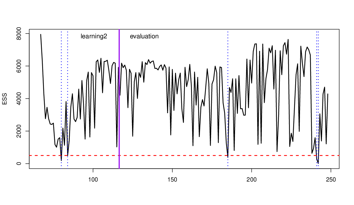
In Figure 2, the realized ESS are plotted over $t=66:248$. The figure also indicates time points when $\text{ESS}_{t}<C=500$ and the MCMC intervention with size $N=10000$ is triggered. With this threshold, we made the intervention five times out of $183\ (t=66:248)$ time points. The total time for this computation is 1266.79 seconds, mainly for the five MCMC interventions. Sensitivity analysis about different values of threshold $C$ can be found in Section S2, where the number of interventions, computational time, and predictive performance are reported.

We assess the accuracy of particle approximation made by the SMC methods for the synthesized predictive distributions, $p(y_{t}|y_{66:t-1},\mathcal{H}_{66:t})$, and the posterior distributions of the calibration parameters, $p(\Phi_{t}|y_{66:t-1},\mathcal{H}_{66:t-1})$, for $t=117:248$. First, we employ the MCMC method repeatedly, using chain size $N=70000$ at each time, to obtain the accurate approximation of the posterior and predictive distributions. Then, we implement the computation by the SMC methods with and without the MCMC interventions and compare their results with the repeated MCMC method.

In Figure 3, we plot the posterior distributions of the location calibration parameter $\theta_{t,0}$, or $p(\theta_{t,0}|y_{66,t-1},\mathcal{H}_{66,t-1})$, for $t=117:248$. Without MCMC interventions, the posteriors computed by the generated particles are biased and degenerated. The fully SMC-based approach is also sensitive to the sudden burst of the inflation rate at $t=242$ (2021/Q2). At this time point, both the agent models and the DLM synthesis significantly fail in prediction, causing a severe particle degeneracy in the sequential analysis. With interventions, the SMC method accurately approximates the target predictive distribution; their median and 90% credible intervals are almost identical to those computed by the MCMC method with the large chain size. We confirmed that the SMC method with interventions can achieve the accurate particle approximation in other posterior plots; see Section S2 for details.

To evaluate the SMC method from the viewpoint of predictive performance, we compute the log predictive density ratios (LPDR) over $t=117:248$, which is defined by

where $p_{\text{MCMC}}(y_{s}|y_{66:s-1},\mathcal{H}_{66:s})$ is the predictive density computed by using the MCMC method repeatedly, and $p(y_{s}|y_{66:s-1},\mathcal{H}_{66:s})$ is the predictive density of interest. If the LPDR is close to $0$, the predictive distribution of interest is as performative as the synthesized predictive distribution computed by the MCMC method. Here, we evaluate the LPDR for the particle approximation of the synthesized predictive density computed by the SMC methods with or without MCMC interventions and the four agent predictive densities. The LPDRs are plotted in Figure 4. Again, without interventions, the approximation errors accumulate gradually over time and critically at the sudden burst of the inflation rate. The MCMC interventions improve approximation accuracy regarding LPDRs at all time points.

In the presence of possible structural changes, power discounting has been utilized in combining the predictive densities (e.g., Zhao et al., 2016). This idea is formalized as the loss discounting framework (LDF) in the context of forecast combination (Bernaciak and Griffin, 2022). Suppose that we have $K$ agent models and their predictive densities, $h_{kt}(y_{t})=p(y_{t}|y_{1:t-1},\mathcal{M}_{k})$, for $k=1:K$. In evaluating the historical performance of the agent models, the LDF uses log-discounted predictive likelihood (LDPL) defined by

where $\gamma_{1}\in(0,1]$ is called the first layer discount factor. If $\gamma_{1}=1$, then the LDPL reduces to the log-marginal likelihood of agent model $\mathcal{M}_{k}$, which is used in the standard Bayesian analysis. The LDPL rates the recent predictive performance of the agent model higher than those in the past, making the model evaluation sensitive to sudden structural changes. Using the LDPLs, the $K$ predictive densities are averaged as

where the weight function, $w_{k}(\cdot)$, depends on the LDPLs. If $w_{k}$ is the expit function, the LDF reduces to the dynamic model averaging (Raftery et al., 2010) and, in the case of $\gamma_{1}=1$, it is the Bayesian model averaging. Bernaciak and Griffin, 2022 proposes two weight functions: softmax and argmax weights defined by

The softmax weights utilize all the $K$ models as in the model averaging, while the argmax weights choose the best model as the final output for prediction. Denote the LDFs with the softmax and argmax weight functions by $\text{LDF}_{s}$ and $\text{LDF}_{a}$, respectively.

The first-layer discount factor, $\gamma_{1}$, is an important tuning parameter to control how much we discount the past predictive performance of the agent models. To emphasize the dependence on $\gamma_{1}$, we write the predictive distribution in the LDF as $p_{\mathrm{LDF}_{\ast}}(y_{t}|y_{1:t-1},\mathcal{H}_{1:t},\gamma_{1})$, where $\ast\in\{s,a\}$. To compare different values of $\gamma_{1}$, we have to obtain multiple predictive distributions with different values of $\gamma_{1}$. These distributions need to be combined in the LDF again. To be precise, we introduce the second-layer discount factor $\gamma_{2}\in[0,1]$, evaluate the LDPL of $p_{\mathrm{LDF}_{\ast}}(y_{t}|y_{1:t-1},\mathcal{H}_{1:t},\gamma_{1})$ for each value of $\gamma_{1}$, and combine the predictive densities using a weight function that is not necessarily the same as one used in the first layer combination. We denote this forecast combination by $\mathrm{LDF}_{\ast_{1},\ast_{2}}$, where $\ast_{1},\ast_{2}\in\{s,a\}$. For example, if we use the softmax weights to combine the predictions made by $\mathrm{LDF}_{a}$, then it is $\mathrm{LDF}_{a,s}$.

Finally, note that we still have to choose the second-layer discount factor, $\gamma_{2}$ carefully. In this study, we set $\gamma_{2}$ to a fixed value. Having extra layers is possible in the general LDF, but is expected to have less impact on the final predictive result.

The LDF can be implemented quickly and fast, but its flexibility is limited since the resulting density is simply the weighted average of $K$ agent predictive densities. Here, we use the idea of the LDF in calibrating the discount factors of the DLM synthesis function of the DBPS, namely, $\beta$ and $\delta$.

Denote the set of $J$ possible values of discount factors by $S=\{(\beta_{1},\delta_{1}),\dots,(\beta_{J},\delta_{J})\}$. At each time $t-1$, for each pair $(\beta_{j},\delta_{j})\in S$, we compute the synthesized predictive distribution, $p(y_{t}|\mathcal{H}_{1:t},y_{1:(t-1)},\beta_{j},\delta_{j})$. Consequently, we have $J$ synthesized predictive distributions, which are combined by using the LDF discount factor, $\gamma$, and the softmax or argmax weight function with argument $\text{LDPL}_{j,t}(\gamma)$ computed by $p(y_{t}|\mathcal{H}_{1:t},y_{1:(t-1)},\beta_{j},\delta_{j})$. We denote this approach by $\text{LDF}_{B,\ast}$, where $\ast\in\{a,s\}$. From the viewpoint of the two-layer LDF, this approach replaces the first-layer density combination with the DBPS.

References

- Aastveit et al., (2023) Aastveit, K. A., Cross, J. L., and van Dijk, H. K. (2023). Quantifying time-varying forecast uncertainty and risk for the real price of oil. Journal of Business & Economic Statistics, 41(2):523–537.
- Baştürk et al., (2019) Baştürk, N., Borowska, A., Grassi, S., Hoogerheide, L., and van Dijk, H. K. (2019). Forecast density combinations of dynamic models and data driven portfolio strategies. Journal of Econometrics, 210(1):170–186.
- Bernaciak and Griffin, (2022) Bernaciak, D. and Griffin, J. E. (2022). A loss discounting framework for model averaging and selection in time series models. arXiv preprint arXiv:2201.12045.
- Billio et al., (2013) Billio, M., Casarin, R., Ravazzolo, F., and Van Dijk, H. K. (2013). Time-varying combinations of predictive densities using nonlinear filtering. Journal of Econometrics, 177(2):213–232.
- Cabel et al., (2022) Cabel, D., Kato, M., McAlinn, K., Sugasawa, S., and Takanashi, K. (2022). Spatially-varying Bayesian predictive synthesis for flexible and interpretable spatial prediction. arXiv preprint arXiv:2203.05197.
- Carter and Kohn, (1994) Carter, C. K. and Kohn, R. (1994). On Gibbs sampling for state space models. Biometrika, 81(3):541–553.
- Casarin et al., (2015) Casarin, R., Grassi, S., Ravazzolo, F., van Dijk, H., et al. (2015). Parallel sequential Monte Carlo for efficient density combination: The DeCo MATLAB toolbox. JOURNAL OF STATISTICAL SOFTWARE, 68.
- Casarin et al., (2023) Casarin, R., Grassi, S., Ravazzolo, F., and van Dijk, H. K. (2023). A flexible predictive density combination for large financial data sets in regular and crisis periods. Journal of Econometrics.
- Chen and Liu, (2000) Chen, R. and Liu, J. S. (2000). Mixture kalman filters. Journal of the Royal Statistical Society: Series B (Statistical Methodology), 62(3):493–508.
- Chen et al., (2018) Chen, X., Irie, K., Banks, D., Haslinger, R., Thomas, J., and West, M. (2018). Scalable Bayesian modeling, monitoring, and analysis of dynamic network flow data. Journal of the American Statistical Association, 113(522):519–533.
- Chernis, (2022) Chernis, T. (2022). Combining large numbers of density predictions with Bayesian predictive synthesis. Preprint.
- Chopin, (2002) Chopin, N. (2002). A sequential particle filter method for static models. Biometrika, 89(3):539–552.
- Doucet et al., (2000) Doucet, A., Godsill, S., and Andrieu, C. (2000). On sequential Monte Carlo sampling methods for Bayesian filtering. Statistics and computing, 10:197–208.
- Frühwirth-Schnatter, (1994) Frühwirth-Schnatter, S. (1994). Data augmentation and dynamic linear models. Journal of time series analysis, 15(2):183–202.
- Genest and Schervish, (1985) Genest, C. and Schervish, M. J. (1985). Modeling expert judgments for Bayesian updating. The Annals of Statistics, pages 1198–1212.
- Gilks and Berzuini, (2001) Gilks, W. R. and Berzuini, C. (2001). Following a moving target—Monte Carlo inference for dynamic Bayesian models. Journal of the Royal Statistical Society: Series B (Statistical Methodology), 63(1):127–146.
- Gordon et al., (1993) Gordon, N. J., Salmond, D. J., and Smith, A. F. (1993). Novel approach to nonlinear/non-Gaussian Bayesian state estimation. In IEE proceedings F (radar and signal processing), volume 140(2), pages 107–113. IET.
- Irie et al., (2022) Irie, K., Glynn, C., and Aktekin, T. (2022). Sequential modeling, monitoring, and forecasting of streaming web traffic data. The Annals of Applied Statistics, 16(1):300–325.
- Johnson and West, (2023) Johnson, M. C. and West, M. (2023). Bayesian predictive synthesis with outcome-dependent pools. arXiv preprint. arXiv:1803.01984.
- Kobayashi et al., (2023) Kobayashi, G., Sugasawa, S., Kawakubo, Y., Han, D., and Choi, T. (2023). Clustering and predicting multiple time series count data via mixture of Bayesian predictive syntheses: Analysis of COVID-19 hospitalisation in Japan and Korea. arXiv preprint. arXiv:2308.06134.
- Liu and West, (2001) Liu, J. and West, M. (2001). Combined parameter and state estimation in simulation-based filtering. In Sequential Monte Carlo methods in practice, pages 197–223. Springer.
- McAlinn, (2021) McAlinn, K. (2021). Mixed-frequency Bayesian predictive synthesis for economic nowcasting. Journal of the Royal Statistical Society: Series C (Applied Statistics).
- McAlinn et al., (2020) McAlinn, K., Aastveit, K. A., Nakajima, J., and West, M. (2020). Multivariate Bayesian predictive synthesis in macroeconomic forecasting. Journal of the American Statistical Association, 115(531):1092–1110.
- McAlinn and West, (2019) McAlinn, K. and West, M. (2019). Dynamic Bayesian predictive synthesis in time series forecasting. Journal of Econometrics, 210(1):155–169.
- Pitt and Shephard, (1999) Pitt, M. K. and Shephard, N. (1999). Filtering via simulation: Auxiliary particle filters. Journal of the American statistical association, 94(446):590–599.
- Prado et al., (2021) Prado, R., Ferreira, M. A., and West, M. (2021). Time series: modeling, computation, and inference. CRC press.
- Raftery et al., (2010) Raftery, A. E., Kárnỳ, M., and Ettler, P. (2010). Online prediction under model uncertainty via dynamic model averaging: Application to a cold rolling mill. Technometrics, 52(1):52–66.
- Rubin, (1988) Rubin, D. (1988). Using the sir algorithm to simulate posterior distributions. Bayesian Statistics, 3:395–402.
- Tallman and West, (2022) Tallman, E. and West, M. (2022). Bayesian predictive decision synthesis. Submitted for publication. arXiv:2206.03815.
- West, (1992) West, M. (1992). Modelling agent forecast distributions. Journal of the Royal Statistical Society: Series B (Statistical Methodology), 54:553–567.
- West and Crosse, (1992) West, M. and Crosse, J. (1992). Modelling probabilistic agent opinion. Journal of the Royal Statistical Society: Series B (Methodological), 54(1):285–299.
- West and Harrison, (1997) West, M. and Harrison, P. J. (1997). Bayesian Forecasting and Dynamic Models. Springer Verlag, 2nd edition.
- Zhao et al., (2016) Zhao, Z. Y., Xie, M., and West, M. (2016). Dynamic dependence networks: Financial time series forecasting and portfolio decisions. Applied Stochastic Models in Business and Industry, 32(3):311–332.
Supplementary Materials for