Funnel-based Control for Reach-Avoid-Stay Specifications
Abstract
The paper addresses the problem of controller synthesis for control-affine nonlinear systems to meet reach-avoid-stay specifications. Specifically, the goal of the research is to obtain a closed-form control law ensuring that the trajectories of the nonlinear system, reach a target set while avoiding all unsafe regions and adhering to the state-space constraints. To tackle this problem, we leverage the concept of the funnel-based control approach. Given an arbitrary unsafe region, we introduce a circumvent function that guarantees the system trajectory to steer clear of that region. Subsequently, an adaptive funnel framework is proposed based on the target, followed by the construction of a closed-form controller using the established funnel function, enforcing the reach-avoid-stay specifications. To demonstrate the efficacy of the proposed funnel-based control approach, a series of simulation experiments have been carried out.
I Introduction
In recent years, there has been significant interest in the study of reach-avoid-stay (RAS) specifications for the safe and reliable operation of autonomous systems. Essentially the system state trajectory should eventually reach a target set while avoiding any unsafe set and respecting state space constraints. Synthesizing controllers for these RAS specifications is an important class of control problem as they serve as building blocks for complex task specifications [1] and enable the design of robust control strategies in safety-critical control problems such as trajectory regulation, motion planning, and obstacle avoidance.
With the onset of the usage of formal languages for specifying complex tasks, symbolic control [2, 3] has emerged as a powerful tool. [4] proposed a fixed-point algorithm as a computational improvement over the abstraction-based methods for control synthesis in a reach-stay scenario. The authors in [5] presented a scalable controller synthesis technique by leveraging the concept of barrier functions in symbolic control. In spite of all these attempts at improving computational efficiency, these approaches still face challenges related to the so-called curse of dimensionality.
In contrast to formal methods, nonlinear control approaches like barrier-based control [6] ensure formal guarantees of safety and stability without the need for state-space discretization. Authors in [7] proposed implementing control Lyapunov-barrier functions to establish sufficient conditions for reach-avoid-stay specifications, specifically in the context of a system experiencing a Hopf-bifurcation. In [8], researchers present a stochastic analog of Lyapunov-barrier functions to characterize probabilistic reach-avoid-stay specifications, taking robustness into account. However, although these methods provide more efficient control synthesis, the reliance on optimization techniques can still lead to increased computational complexity, making barrier function-based methods computationally demanding, especially for large and high-dimensional systems.
On the other hand, the funnel-based control approach [9] offers the distinct advantage of designing a closed-loop control scheme satisfying a required tracking performance. Owing to the computationally tractable nature of funnel-based control, numerous successful applications have been reported in the literature [10]. From solving tracking control problems for unknown nonlinear systems [11] to handling multi-agent systems subjected to complex task specifications [12], researchers have demonstrated its efficacy in a wide range of control problems. Moreover, as the feedback control algorithm actively adjusts the system’s trajectory to guide it towards the target, it has been effective in enforcing reachability specifications, i.e., reaching a target while respecting state space constraints [13, 14].
However, active obstacle avoidance using funnel-based control can be a challenging problem. One of the main difficulties lies in designing accurate and efficient funnel representations to ensure safe navigation around obstacles while maintaining reach-avoid-stay specifications. In [15], authors consider a pre-established trajectory around the obstacles and redefine the problem as implementing control funnel functions for path following. Although this approach ensures that the system remains in a safe region around the reference trajectory, it fails to utilize the inherent ability of funnel constraints to avoid obstacles.
This paper puts forward, for the very first time, a novel approach to integrate avoid-specifications within the funnel-based control framework. By adapting the funnel constraints, the closed-form control law dynamically adjusts the robot’s trajectory to avoid any general unsafe set while maintaining the desired performance criteria. The effectiveness of this approach in satisfying reach-avoid specifications is further demonstrated through simulation studies, highlighting its potential to enhance the capabilities of robotic systems in navigating complex environments.
II Preliminaries and Problem Formulation
II-A Notations
The symbols , , , and denote the set of natural, real, positive real, and nonnegative real numbers, respectively. We use to denote a vector space of real matrices with rows and columns. To represent a column vector with rows, we use . We represent the Euclidean norm using . For and , we use to represent open interval in . For and , we use to denote close interval in . To denote a vector with entries , we use , where denotes -th element of vector . A diagonal matrix in with diagonal entries is denoted by . Given sets , , the Cartesian product of the sets is given by . Consider a set , its projection on th dimension, where , is given by an interval , where and . We further define the hyper-rectangle . We denote the empty set by . The space of bounded continuous functions is denoted by . Given a compact set , represents the interior of the set and represents the boundary of . and are smooth approximations of the non-smooth and functions, defined as, and , respectively. The sign function is defined as .
II-B System Definition
Consider the following control-affine nonlinear system:
| (1) |
where and are the state and control input vectors, respectively. The state space of the system is defined by the closed and connected set . The functions and satisfy Assumption 1.
Assumption 1
and are locally Lipschitz, and is positive definite for all .
II-C Problem Formulation
The paper considers the desired behavior of the system , in (1), defined in the form of reach-avoid-stay specifications.
Let the compact and connected set be the target set, the set be an unsafe region containing unsafe sets defined as, , where is a convex, compact, and connected set, representing, the th unsafe set. Thus, in general, the unsafe region , although necessarily compact, can be disconnected and nonconvex.
Now, we will formally define the main controller synthesis problem considered in this work.
Problem II.1
We approach this problem using a funnel-based control strategy to enforce reachability specification (Section III) and then dynamically modifying the funnel around the unsafe region to ensure that the system trajectory avoids the unsafe region while respecting the state constraints (Sections IV-V).
Remark II.2
If is of any arbitrary shape, we redefine the state space as the hyper-rectangle and expand the unsafe region . Here, represent the projection of set on the th dimension. Note that, adding to the unsafe set and following Algorithm 1 in Section V, enforces stay specifications for an arbitrary state-space .
III Controller for Reachability Specification
In this section, we formulate a funnel-based control strategy aimed at guaranteeing that the system’s trajectory adheres to the reachability specifications, i.e., given a target set and a given initial position , the controlled trajectory will eventually reach the target set in finite time. To solve the reachability problem, we leverage the funnel-based control approach [9]. We first define the funnel constraints over the trajectory as follows:
| (2) |
where , and . is the continuously differentiable, positive and non-increasing funnel function defined as:
| (3) |
with , and governs the lower bound of convergence rate.
The above choice of , , and ensures that the initial state of the system is within and by the aforementioned choice of , as . Thus, enforcing system state inside funnel constraints (2) ensures reachability. An example of a funnel designed for enforcing reachability specification is shown in Figure 1 (a).
To design a controller enforcing condition (2), we first define the normalized error , as
| (4) |
Now the corresponding constrained region can be represented by . Next the normalized error is transformed through a smooth and strictly increasing transformation function with . The transformed error is then defined as , where
| (5) |
By this definition, if the transformed error is bounded, then the normalized error is confined within the constrained region and the state adheres to (2). We also define with
| (6) |
where .
Now, in Theorem III.1, we propose a control strategy such that the state trajectory is constrained within the funnel.
Theorem III.1
Consider the control-affine system given in (1) with Assumptions 1. Given a target set , the funnel constraints and (2), the control strategy
| (7) |
will drive the state trajectory , to the target set in finite time, i.e., . Here, is any positive constant, , with , , , and are defined in (4), (5), and (6), respectively.
Proof:
The proof follows on similar grounds as that of Theorem IV.3 and is omitted here due to space constraints. ∎
IV Extension to Reach-Avoid-Stay Specification
In this section, we begin by exploring the integration of avoidance of unsafe regions within the funnel-based control framework. Subsequently, we present an adaptive funnel design strategy that enables the successful accomplishment of reach-avoid-stay tasks.

IV-A Design of Circumvent Function
Consider an unsafe region with compact, connected and convex sets , for . We propose to introduce the avoid specifications through a circumvent function , .
Remark IV.1
Note that although we are putting an assumption on to be convex and connected, the general unsafe zone can be concave and disconnected. This will further be elaborated upon in Section V.
First, given an initial state , we obtain the time range over which the system trajectory , on application of the control law (7) to satisfy the reachability specification, intersects with the th unsafe set , and is given by, and .
Consider the first unsafe set that the system trajectory intersects be , where
| (8) |
Following this, we will discuss the introduction of the circumvent function and adaptive funnel design to steer clear of . The subsequent extension to deal with the entire unsafe region with multiple disconnected concave unsafe sets is presented in Section V.
Further, note that the system’s trajectory enters the unsafe zone , if and only if , such that . Hence, to satisfy the avoid specification, it is sufficient to introduce the circumvent function only in one dimension , given by
| (9) |
where and is the projection of in the th dimension. Note that, may not be unique and in the case, the trajectory enters the projections of in multiple dimensions at the same time, the function returns randomly from those multiple alternatives. The advantage of this random selection will be discussed in Section V.
We also have the liberty to choose between modifying either the upper or the lower constraint boundary of the funnel. Unless the scenario where or , where the circumvent function should necessarily be introduced in the lower and upper constraint boundary, respectively (it can be visualized as the scenario of a wall-shaped obstacle, where there is no space between the state space boundary and the obstacle at one end), we randomly choose between the two options. Although an optimal alternative can be easily chosen, the advantage of random picking is discussed in Section V.
We define the circumvent function on lower constraint boundary for as:
| (10) |
where, , , and is a tolerance factor. The function is active in the time range when the system trajectory avoids . The governs how far from should the trajectory stay clear. is a small positive constant and determines the smoothness of the circumvent function.
Similarly, we define a circumvent on the upper constraint boundary as
| (11) |
with and the rest of the parameters are the same as above.
An example of the introduction of the circumvent function on the lower constraint of a funnel is shown in Figure 1 (b).
IV-B Adaptive Funnel Design
Given a target set and obstacle , choose a point . Now, according to (2), construct the funnel and to satisfy the reachability specification. As defined in the previous subsection, we characterize the obstacle using the circumvent function , and now, we incorporate it into the funnel design. To solve Problem II.1, we propose the following adaptive funnel constraints.
| (12) | |||
| (13) |
The modifications in the constraints of the funnel are captured by a continuously differentiable update function, . The adaptive law governing the dynamics of the update function is defined as:
| (14) |
where if introduced on lower constraint and if introduced on upper constraint , with as a tolerance factor. acts as a trigger, activating the first part of the update function only when reach-avoid specifications are conflicting with a tolerance of and is given by:
where controls the deviation of the funnel around the circumvent function.
Further, the non-smooth function is approximated by the smooth function . When the conflict is resolved, becomes 0 and the second part decays exponentially back to zero with a rate of decay governed by constant . An example of how the circumvent function modifies the funnel is shown in Figure 1 (c).
Let us now define , , , and .
Lemma IV.2
.
Proof:
From definitions (3),(10), and (11), one has and . Thus, to show that and , it is sufficient to show that .
Since and is a bounded tolerance, is also continuous and bounded. Further, . Hence, .
Now, depending on the sign of , consider the two cases and look at and elementwise:
Case I. [] This implies that and . Thus, which implies for .
Case II. [] This implies that and .
| (15) |
We will prove the boundedness of by contradiction. Let (converges to zero). Then taking its derivative w.r.t time , we can say . From the fact that , we have . However, from (15) we can observe that if then . This leads to a contradiction. Therefore, (does not converge to zero) and consequently, for .
To further prove the boundedness of , we will again use contradiction. Let . Now, since is bounded and is a finite constant, . But and are contradictory. Hence,
Let . Similarly, since is bounded and is a finite constant, . But and are contradictory. Hence, .
Therefore, in both cases we reach the same conclusion, .
∎
IV-C Controller Design
In this section, utilizing the adaptive funnel, discussed in the previous section, we derive the funnel control law to solve Problem II.1. The controller design is done in three stages.
Stage I. Given an initial state and target state , construct the funnel constraints (2) that guide the system trajectory to the target , as discussed in Section III.
Stage II. Given the unsafe region , obtain as shown in (8) and compute the circumvent function according to (10) or (11). Now modify the funnel around the circumvent function, as discussed in Section IV-B, and determine the adaptive funnel framework, defined by and .
Stage III. For the modified funnel, we define the normalized error as
| (16) |
The corresponding constrained region can be represented by: . The transformed error is defined as:
| (17) |
We also define a diagonal matrix, , as
| (18) |
Now, in Theorem IV.3, we propose a control strategy such that the state trajectory satisfies reach-avoid-stay specifications.
Theorem IV.3
Consider a nonlinear control-affine system given in (1), assigned a reach-avoid task expressed mathematically through (3) and (10, 11) respectively. If the initial state is within the modified funnel (Section IV-B), then the control strategy
| (19) |
will drive the state trajectory to the target while avoiding the unsafe set (8) and adhering to state constraints, i.e., and . Here, is any positive constant, , , and are defined in (16), (17), and (18), respectively.
Proof:
The proof comprises three steps. First, we show that there exists a maximal solution for the normalized error , which implies that remains within in the maximal time solution interval . Next, show that the proposed control law (19) constraints to a compact subset of . Finally, prove that can be extended to .
Before proceeding let us introduce two lemmas:
Lemma IV.4
[16, Theorem 54] Consider the IVP . Assume is
- 1.
locally Lipschitz on , for each
- 2.
piecewise continuous on for each fixed
Then there exists a unique and maximal solution where .
Lemma IV.5
Continuing with the proof.
Substituting the controller (19) in the system dynamics (1), we obtain the closed-loop dynamics:
and substituting the above equation in , we obtain
Consider the augmented state and its derivative as
Since the initial state is within the updated funnel, the initial normalized error is within the constrained region . Note, that is an open and bounded set. Further, define , which is a non-empty open and bounded set. Thus, is also a non-empty open and bounded set and the initial condition of the augmented state satisfy . Therefore, we have the following initial value problem at hand: .
We can see that (17), (18) and , defined on , are locally Lipschitz continuous in . Further, according to Assumption 1, is also Lipschitz continuous on in . Therefore, we can conclude that is locally Lipschitz continuous on in .
Hence, according to Lemma IV.4, there exists a maximal solution of the IVP in the time interval :
Step 2. Based on Step 1, we know
Consider the following positive definite and radially unbounded Lyapunov function candidate: .
Differentiating with respect to time and substituting , and system dynamics (1), we obtain:
Now employ the control strategy (19), we get
where . We will look at the boundedness of the two terms in separately. First, we know is a continuous function of and , an open and bounded set. Thus, by applying the extreme value theorem, we can infer . Finally, from Lemma IV.2 we know that is also bounded. Hence, .
Now add and substract , where
Therefore, we can conclude that there exists a time-independent upper bound to the transformed error , i.e., .
Further, we know from (17) that . Taking inverse, we can bound the normalized error as:
Therefore, by employing the control law (19), we can constrain to a compact subset of as:
| (21) |
where, and
Step 3. Finally, we prove that can be extended to .
We know that , where is a non-empty compact subset of .
Consequently we can conclude that also evolves in a compact set:
| (22) |
Define the compact set and note that . Therefore, there is no such that .
However, if then according to Lemma IV.5, such that . This leads to a contradiction! Hence, we conclude that can be extended to , i.e., satisfies the funnel constraints in (2) .
In conclusion, the satisfaction of (2) is guaranteed for all time when we employ the control strategy (19). ∎
Remark IV.6
From Assumption 1, we know is invertible. (21) entails that is bounded. And by definitions (16) and (18), and are also bounded. Further, from Lemma IV.2, also . Finally, all the non-smooth functions in the revamped funnel design in Section IV-B are replaced by their smooth approximations. Hence, the control law (19) is well-defined, i.e., continuous, smooth, and bounded.
Remark IV.7
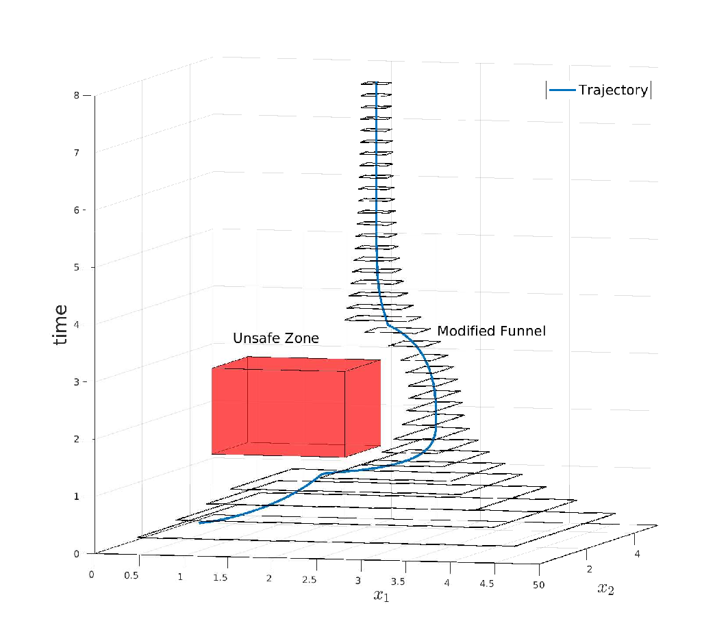
In Figure 2, we present a 3D visualization of a scenario where and the modified funnel circumvents around the unsafe set , providing a safe path for the trajectory to reach the target while staying clear of .

V Extension to Tackle General Unsafe sets
Given the unsafe region with connected convex sets, we first choose (8). The control law (19) ensures that the controlled state trajectory reaches the target while avoiding this . Now, to address for , we iterate through this procedure until the controlled system trajectory stays entirely clear of the unsafe region .
Further, in each iteration, for defining the function, we have a certain degree of randomness. We randomly select from all the possible alternatives (9). Moreover, we also randomly choose whether to introduce in the lower constraint (10) or upper constraint (11), as discussed in Section IV-A. This randomness allows exploration of all the paths around unsafe regions, thus resulting in a higher probability of obtaining a closed-form controller satisfying reach-avoid-stay specifications for complex environments. The algorithm is presented in Algorithm 1.
Algorithm 1 Extension for general unsafe region
Input:
Output:
- 1.
Given , choose and construct funnel constraints to enforce reachability (2)
- 2.
Apply control law (7) to drive the controlled trajectory to the target while remaining within the state limits.
- 3.
while true do
- 4.
- 5.
-
Apply control law (19) and obtain the controlled trajectory .
-
- 6.
-
if ()
-
- 7.
-
return
-
- 8.
-
end
-
- 9.
end
Corollary V.1
Thus, given a system in (1), target set in the state space and unsafe region , termination of the Algorithm 1 defines an adaptive funnel framework and provides us a well-defined closed-form control law (19) that will guide the system trajectory to the target while avoiding the unsafe region, enforcing reach-avoid-stay specifications.
A simulation study illustrating the efficacy of the algorithm in solving reach-avoid-stay specifications in a multi-obstacle environment is presented in the next section.
VI Simulation Results
Consider a three-wheeled omnidirectional robot operating on a 2-D plane. The Kinematic model of the mobile robot is expressed as:
| (23) |
where captures the robot’s position and orientation respectively. The control inputs, u, v, and are linear velocities in the x and y direction of the robot frame and the angular velocity respectively. Note that the robot dynamics satisfy Assumption 1.
We ran the tests for a 2D arena with two wall obstacles and a circular obstacle. The funnel for guiding the robot towards the target is shaped according to (3) with the following parameters: and for . and represents the and coordinates respectively. For the circumvent function (10) or (11), we define , and for all the obstacles. Finally the adaptive law (14) is established with , and .
The simulation results with three different initial states are depicted in Figure 3.
VII Conclusion
In this work, we consider the controller synthesis problem for reach-avoid-stay specification. Given state space constraints, obstacles, and targets, we first proposed the introduction of a circumvent function and construction of an adaptive funnel framework. We have then derived a closed-form control law ensuring that the trajectories of a nonlinear system reach target while avoiding all the unsafe regions and respecting state-space constraints, thus, enforcing reach-avoid-stay specifications. Finally, the efficacy of the proposed approach is demonstrated through simulation studies.
References
- [1] M. Kloetzer and C. Belta, “A fully automated framework for control of linear systems from temporal logic specifications,” IEEE Transactions on Automatic Control, vol. 53, no. 1, pp. 287–297, 2008.
- [2] P. Tabuada, Verification and control of hybrid systems: a symbolic approach. Springer Science and Business Media, 2009.
- [3] G. Reissig and M. Rungger, “Feedback refinement relations for symbolic controller synthesis,” in 53rd IEEE Conference on Decision and Control, pp. 88–94, 2014.
- [4] Y. Li and J. Liu, “Robustly complete synthesis of memoryless controllers for nonlinear systems with reach-and-stay specifications,” IEEE Transactions on Automatic Control, vol. 66, no. 3, pp. 1199–1206, 2021.
- [5] S. S. David, B. Jay, Saharsh, C. Jeel, S. Adnane, and J. Pushpak, “Scalable distributed controller synthesis for multi-agent systems using barrier functions and symbolic control,” in IEEE 62nd Conference on Decision and Control (CDC), 2023.
- [6] A. D. Ames, X. Xu, J. W. Grizzle, and P. Tabuada, “Control barrier function based quadratic programs for safety critical systems,” IEEE Transactions on Automatic Control, vol. 62, no. 8, pp. 3861–3876, 2017.
- [7] Y. Meng, Y. Li, and J. Liu, “Control of nonlinear systems with reach-avoid-stay specifications: A Lyapunov-barrier approach with an application to the Moore-Greizer model,” in American Control Conference (ACC), pp. 2284–2291, 2021.
- [8] Y. Meng and J. Liu, “Sufficient conditions for robust probabilistic reach-avoid-stay specifications using stochastic Lyapunov-barrier functions,” in American Control Conference (ACC), pp. 2283–2288, 2022.
- [9] C. P. Bechlioulis and G. A. Rovithakis, “Robust adaptive control of feedback linearizable MIMO nonlinear systems with prescribed performance,” IEEE Transactions on Automatic Control, vol. 53, no. 9, pp. 2090–2099, 2008.
- [10] X. Bu, “Prescribed performance control approaches, applications and challenges: A comprehensive survey,” Asian Journal of Control, vol. 25, no. 1, pp. 241–261, 2023.
- [11] P. K. Mishra and P. Jagtap, “On controller design for unknown nonlinear systems with prescribed performance and input constraints,” in Eighth Indian Control Conference (ICC), pp. 212–217, 2022.
- [12] F. Chen and D. V. Dimarogonas, “Funnel-based cooperative control of leader-follower multi-agent systems under signal temporal logic specifications,” in European Control Conference (ECC), pp. 906–911, 2022.
- [13] F. Mehdifar, C. P. Bechlioulis, and D. V. Dimarogonas, “Funnel control under hard and soft output constraints,” in IEEE 61st Conference on Decision and Control (CDC), pp. 4473–4478, 2022.
- [14] P. Jagtap and D. Dimarogonas, “Controller synthesis against omega-regular specifications: A funnel-based control approach,” 2023.
- [15] H. Ravanbakhsh, S. Aghli, C. Heckman, and S. Sankaranarayanan, “Path-following through control funnel functions,” in IEEE/RSJ International Conference on Intelligent Robots and Systems (IROS), pp. 401–408, 2018.
- [16] E. D. Sontag, Mathematical control theory: deterministic finite dimensional systems, vol. 6. Springer Science and Business Media, 2013.
