Knowledge-based Multiple Adaptive Spaces Fusion for RecommendationConference: Seventeenth ACM Conference on Recommender Systems; September 18–22, 2023; Singapore, SingaporeSeventeenth ACM Conference on Recommender Systems (RecSys ’23), September 18–22, 2023, Singapore, SingaporePrice: 15.00DOI: 10.1145/3604915.3608787ISBN: 979-8-4007-0241-9/23/09CCS: Information systems Recommender systems
Abstract.
Since Knowledge Graphs (KGs) contain rich semantic information, recently there has been an influx of KG-enhanced recommendation methods. Most of existing methods are entirely designed based on euclidean space without considering curvature. However, recent studies have revealed that a tremendous graph-structured data exhibits highly non-euclidean properties. Motivated by these observations, in this work, we propose a knowledge-based multiple adaptive spaces fusion method for recommendation, namely MCKG. Unlike existing methods that solely adopt a specific manifold, we introduce the unified space that is compatible with hyperbolic, euclidean and spherical spaces. Furthermore, we fuse the multiple unified spaces in an attention manner to obtain the high-quality embeddings for better knowledge propagation. In addition, we propose a geometry-aware optimization strategy which enables the pull and push processes benefited from both hyperbolic and spherical spaces. Specifically, in hyperbolic space, we set smaller margins in the area near to the origin, which is conducive to distinguishing between highly similar positive items and negative ones. At the same time, we set larger margins in the area far from the origin to ensure the model has sufficient error tolerance. The similar manner also applies to spherical spaces. Extensive experiments on three real-world datasets demonstrate that the MCKG has a significant improvement over state-of-the-art recommendation methods. Further ablation experiments verify the importance of multi-space fusion and geometry-aware optimization strategy, justifying the rationality and effectiveness of MCKG.
Keywords:
Knowledge Graph, Recommender Systems, Multiple Space Fusion, Geometry-aware Optimization Strategy1. Introduction
Recommender systems (RSs) have shown great potential in solving the information explosion problem and enhancing the user experience in various online applications (Sun et al. 2020). In a variety of scenarios, knowledge graphs (KGs) can be utilized to offer fundamental background knowledge as well as rich structural information. To fully utilize KG, existing knowledge-enhanced recommendation methods (Qu et al. 2019; Huang et al. 2018; Wang et al. 2018a; Wang et al. 2021a; Chen et al. 2020) strive to build more effective neural networks to integrate the semantics of KG.
Although these techniques can significantly enhance the embeddings of users and items, they are entirely designed based on Euclidean space without considering curvature. Recent studies (Bachmann et al. 2020; Peng et al. 2021; Zhang et al. 2022a) have revealed that a tremendous data exhibits the highly non-Euclidean properties, especially the data that presents tree-likeness or cyclic structures. For instance, the KG data are diverse and include a variety of structures. As shown in Figure 1, there are interactions between the user and items, which can be further connected to more entities. Owing to such high-order relationship (Wang et al. 2019a), knowledge-aware methods have the ability to provide accurate recommendations. Essentially, such interactions can be seen as tree structures or cyclic structures. In such situations, Euclidean space methods suffer from severe distortion when depicting these structures (Chami et al. 2019; Sala et al. 2018a). Furthermore, recent studies (Liu et al. 2019; Gu et al. 2019) have demonstrated that geometric spaces with constant non-zero curvature can enhance representation performance when the underlying graph structures of the data follow particular patterns. Specifically, the hyperbolic space is more suitable for modeling tree-structured data, while the spherical space is superior for representing cyclic patterns.

Since complex KG usually have varied structures coupled together, choosing the ideal space is especially tricky. Constant curvature space methods (Chen et al. 2022; Tai et al. 2021; Bachmann et al. 2020; Grattarola et al. 2018) just project entities to a single space, as a result, they fail to completely express the sophisticated structures of KG. Recently, some mixed-curvature space works (Gu et al. 2018; Han et al. 2020; Wang et al. 2021b) merge distinct spaces, aiming to characterize various structures. Unfortunately, how to find the most effective combination of these manifolds is also a challenging task. The simplest method (Zhang et al. 2022b) is to list all possible combinations and choose the one that best utilizes these geometry. Obviously, this method would be efficient but impractical due to the time-consuming and low-scalability (Skopek et al. 2019). Another solution (Chen et al. 2022) is to treat the curvature as a trainable parameter, aiming to learn the optimal curvature from the training data. However, there are still the following issues: 1) the constraints of model parameters depend on the changes of curvature. Once the curvature varies (e.g., from negative to positive), parameters may no longer satisfy the constraints. As a result, the internal structure of manifold will be destroyed, thus unable to obtain high-quality embeddings. 2) Since the manifolds belong to different spaces, i.e., , directly operating on various manifolds without considering the heterogeneity is problematic. For instance, the global distance computation just sums up the distances without distinguishing the importance of various manifolds.
Motivated by the above observations, in this paper, we propose a knowledge-based multiple adaptive spaces fusion method for recommendation (MCKG). Unlike existing methods (Chen et al. 2022; Tai et al. 2021; Sun et al. 2021; Yang et al. 2022) that solely consider a specific manifold, we introduce a unified space that is compatible with the hyperbolic, euclidean and spherical spaces. Note that the unified space can interpolate smoothly between all geometries of constant curvature, thus the internal structure of the manifold is preserved when training curvature. To break the limitation of the single space’s expression ability, we further integrate multiple unified spaces to more accurately capture the structural information on a global level. On the other hand, we propose a geometry-aware optimization strategy that enables the pull and push processes benefited from both hyperbolic and spherical spaces. Specifically, in hyperbolic space, we set smaller margins in the area near to the origin, which is conducive to distinguishing between highly similar positive items and negative ones. At the same time, we set larger margins in the area far from the origin to ensure that the model has sufficient error tolerance. Conversely, in spherical space, the geometry-aware strategy assigns larger margins near to the origin and smaller margins far from the origin. Empirically, we conduct comprehensive experiments on the three benchmark datasets, the results show that MCKG outperforms the state-of-the-art recommendation methods. In summary, this work makes the following contributions:
- •
To the best of our knowledge, this is the first work to apply multiple adaptive spaces fusion for knowledge-enhanced recommender systems.
- •
We present a knowledge-based multiple adaptive spaces fusion method for recommendation. To obtain the high-quality embeddings for recommendation, we introduce the unified space to describe the complex structures of KG, then further fuse multiple subspaces in an attention manner. Finally, our proposed geometry-aware optimization strategy is the first work that considers the properties of both hyperbolic and spherical spaces.
- •
We conduct extensive experiments on the three benchmark datasets, results show that MCKG outperforms the state-of-the-art recommendation methods.
2. PRELIMINARIES AND PROBLEM FORMULATION
2.1. Mathematical Concepts
In this subsection, we summarize preliminary notations for readers to better understand this paper.
Manifold: A manifold of dimension is a topological where each point’s neighborhood can be approximated by euclidean space . For example, the earth can be modeled by the spherical space, and its local place can be estimated by . The notion of manifold is a generalization of the notion of surface.
Tangent space: For each point , the tangent space of at is defined as a -dimensional space estimating around x at a first order.
Geodesics distance: Geodesics distance is the the generalization of a straight line in the Euclidean space, which indicates the shortest path between pairs of points.
Exponential map: The exponential map carries a vector of a point to the manifold , i.e., Exp by traveling a fixed distance along the geodesic defined as with direction . Each manifold has its own manner to design the exponential maps.
Logarithmic map: The logarithmic map is the reverse operation of the exponential map, which projects a point on the manifold back to the tangent space of another point , i.e., Log. Similar to Expx, different manifolds correspond to their distinct logarithmic map.
2.2. Constant Curvature Spaces
With the constant sectional curvature , the three types of manifolds are defined as follows:
| (1) |
where the represents the inner product:
| (2) |
Because hyperbolic or spherical spaces are not vector spaces, the vector operations (e.g., addition, subtraction and scalar multiplication) cannot be achieved. Therefore, we need to convert non-Euclidean spaces into tangent spaces for corresponding vector calculations. Specifically, the tangent space at point on is a -dimensional Euclidean space that approximates around :
| (3) |
As mentioned in the previous section, the mapping between manifold and its tangent space can be achieved by the exponential and logarithmic operations.
To connect vectors in tangent spaces, the parallel transport (Helgason 1978) defines a manner of transporting the local geometry along smooth curves that preserves the metric tensors. Specifically, for vector and , the parallel transport carries a vector in along the geodesic from to .
2.3. Mix-Curvature Spaces
Since the constant curvature space is only suitable for a certain geometric structure, mix-curvature methods (Bachmann et al. 2020; Gu et al. 2018; Zhang et al. 2022b; Kochurov et al. [n.d.]; Skopek et al. 2019) expect to match the complicated geometry of data thus provide higher quality representations. To capture a wider range of curvatures, mix-curvature methods propose embeddings into product spaces (Gu et al. 2018) where each component has constant curvature. Formally, assuming a series of distinct constant curvature spaces , the mix-curvature manifold are defined as:
| (4) |
where the denotes Cartesian product.
2.4. Problem Formulation
We follow the recommendation setting (Wang et al. 2018a; Wang et al. 2019a; Chen et al. 2022). Let and denote the sets of users and items, respectively. The user-item interaction matrix is defined based on the users’ implicit feedback, where the value of denotes that there is an interaction between user and item ; otherwise . We also have a knowledge graph available, which consists of massive entity-relation-entity triplets , where , , and describe the head, relation, and tail of knowledge triples, and and denote the set of entities and relations. Given the user-item interactions and the item-side KG, the recommendation task is to train a RS model calculating the probability that the user will click item .
3. METHOD
In this section we present the MCKG model in Figure 2. First, we introduce the -Stereographic manifold and the extraction of high-order information on a single manifold. Then, we fuse the each adaptive subspaces to fully capture the global structural information. Finally, we propose a novel geometry-aware optimization strategy to be compatible with both hyperbolic and spherical spaces.
| Name | Operation |
|---|---|
| Addition | |
| Multiplication | |
| Concatenate | |
| Dot Product | |
| Geodesics Distance | |
| Exponential Map | |
| Logarithmic Map |
3.1. Unifying All Curvatures
We adopt -Stereographic model (Bachmann et al. 2020) as the base manifold, which is a unification of constant curvature manifolds: , and . The model is a Riemannian manifold with constant sectional curvature and dimension :
| (5) |
where is conformal metric tensor at point . For the -Stereographic model, the optimization step changes the geometry of space and the constraints of parameters, which also depend on the curvature. Fortunately, when we use curvature as a trainable parameter, the model can interpolate smoothly between all geometries of constant curvature, and the detailed proof process can refer to paper (Bachmann et al. 2020).
The basic operations of the unified space are summarized in Table 1, but the trigonometric functions in Table 1 are not complete, here we complement its definition.
| (6) |
| (7) |
3.2. High-Order Information Extraction
Since the initial embeddings are in Euclidean space, we explicitly encode the Euclidean embeddings onto the unified space before feeding the subsequent layers. Denote the initial user, item and relation embeddings as , and respectively, then the exponential maps are applied:
| (8) |
We present a relational attention function as follows to describe user’s interest:
| (9) |
Intuitively, means the importance of relation to user . The neighboring information can be continuously aggregated based on . Specifically, the neighborhood embedding of entity is defined as
| (10) |
where denotes the selected neighbors of , the is the normalized user-relation score, and means the basic exponential function.
The key idea of Graph Convolution Network (GCN) is to aggregate feature information from a node’s neighbors. Obviously, feeding the entire knowledge graph to model will greatly increase the computational burden. To this end, we assign a fixed size receptive field for each node to control the amount of calculation. After getting the neighborhood representation, we aim to represent target node at the next layer. There are three kinds of aggregators:
- •
GCN Aggregator (Niepert et al. 2016) adds the two representations and performs a nonlinear transformation, and it can be formulated as
(11) where is LeakyRelu activation function, and b represent the weight matrix and bias respectively, and denote the multiplication and addition as mentioned in Table 1.
- •
GraphSage Aggregator (Hamilton et al. 2017) concatenates the two representations, then fed to the activation function:
(12) where the is the concatenation operation.
- •
Neighbor Aggregator (Wang et al. 2019a) takes the neighborhood representation of entity as the output representation, and it can be formulated as
(13)
The embeddings at different layers capture different semantics. E.g., the first layer focuses on items that users has directly interacted with, the second layer emphasizes overlapping items between users, and the higher-layers can capture higher-order information (Wang et al. 2019b). After layers aggregation, we further combine the embeddings obtained at each layer to form the final item representations:
| (14) |
3.3. Multiple Spaces Fusion
Since the complicated structures are not evenly distributed over the entire graph, even if a single space can learn the ideal curvature , it is still not capable of fully modeling the entire graph. Now we consider a sequence of manifolds , where the item (user) embedding in the -th subspace is denoted as . To accurately capture the global structural information, we design a fusion mechanism by aggregating subspace embeddings. First, we take the average of subspace representations as the global fused embeddings , then we concatenate the average value and the original subspace embedding to obtain the new subspace embedding:
| (15) |
As a result, the new embeddings take into account the global information, which is not limited to the current space. Finally, we further integrate the series of subspaces in an attention-enhanced manner. In other words, we calculate the global distance in an attention manner. Formally, the global distance between user and item is the weighted sum of the distances in each subspace:
| (16) |
where the represents geodesics distance as mentioned in Table 1, and the is defined as:
| (17) |
Here the importance of a user-item pair is the sum of the influence of and . Due to the and are the entity level subspace attention, the weights can be pre-trained as follows:
| (18) |
where the and are matrices of size 1 × M and each entry stands for the importance of the corresponding subspace.
| (19) |
In summarize, the multiple spaces fusion method has the following advantages:
- •
Different from existing mixed curvature methods (Zhang et al. 2022b; Kochurov et al. [n.d.]; Gu et al. 2018; Wang et al. 2021b) manually combine various manifolds, we adopt the adaptive curvature spaces instead of constant curvature spaces, e.g., , and .
- •
To accurately model the complex structure of the graph, we further integrate each subspace in an attention-enhanced manner from a global perspective.
3.4. Geometry-aware Optimization Strategy
The margin-based ranking loss has shown to be quite beneficial for non-Euclidean recommendation models (Sun et al. 2021; Yang et al. 2022). This loss seeks to distinguish user-item pairs up to a specified margin into positive and negative samples, once the margin is satisfied the pairs are regarded as well separated. Specifically, for each user we sample a positive item and a negative item , and the margin loss is defined as
| (20) |
where the denotes the global distance in unified space as mentioned in equation (16), is the margin between and . As a result, positive items are pulled closer to user while negative items are pushed outside the margin.
However, it is still unclear how to pick a suitable margin. HGCF (Sun et al. 2021) sets the margin to a constant, this action ignores the exponentially expansive geometric properties of hyperbolic spaces. Furthermore, to emphasize the importance of modeling tail items, HICF (Yang et al. 2022) sets a greater margin in the vicinity of the hyperbolic origin and a smaller margin elsewhere. Although this method can alleviate the power-law distribution to a certain extent, it will hurt the model performance. E.g., in hyperbolic spaces, the space capacity of the area near the origin is extremely narrow, thus a smaller margin is beneficial to distinguish highly similar entities. While in areas far away from the origin, we prefer a greater margin because the room is spacious enough. On the other hand, in spherical spaces, the origin area is relatively spacious, but the boundary area is narrow. Therefore, we expect assigning larger margins to the area closer to the spherical origin, and smaller margins to the area farther from the spherical origin.
Motivated by the above considerations, we aim to devise a geometric-aware optimization strategy which can benefit from both hyperbolic and spherical spaces. Paper (Sala et al. 2018b) discovered an intriguing phenomenon: when entities and progressively moves away from the origin in hyperbolic space, the ratio is getting greater. Obviously, the reason is that the numerator (distance) grows significantly faster than the denominator (radius) in hyperbolic spaces. On the contrary, as entities and move away from the spherical origin, the ratio will gradually become smaller. Surprisingly, the change trend of this ratio is in line with our expectations for the margin. Inspired by these observations, we carefully design the margin as follows:
| (21) |
where is the sigmoid function for normalization, and we maintain the constant for better parameter tuning. Then the is utilized to replace the in equation (20). As a result, the margin will increase as it slowly departs from the origin in hyperbolic spaces, and in spherical spaces it’s the exact opposite. To summarize, either in the hyperbolic or spherical spaces, our model have the ability to perceive the spatial structures and learn the ideal margin.
It is worth mentioning that HICF (Yang et al. 2022) aims to improve the attention of tail items in hyperbolic space, thus the margin is set as follows:
| (22) |
Therefore, it assigns larger margins in narrower areas and smaller margins in spacious areas, exactly the opposite of what we expect. We will compare the performance of various margins in Section 4.3.1.
3.5. Time Complexity Analysis
As we can see, the layer-wise propagation is the core operation in MCKG. Let denotes the number of user-item interactions, for the -th layer, the matrix multiplication computational complexity is , where represents the item neighbor sampling size, and denotes the current transformation size. As a result, the overall time complexity of our proposed model is , where is the number of manifolds, and denotes the number of graph convolution layers. Parameter setting details will be introduced in Section 4.1.4.
4. EXPERIMENTS
In this section, we introduce the experimental settings, and perform extensive comparative experiments with the state-of-the-art models. Then we conduct comprehensive ablation studies to verify the designs in MCKG and reveal the reasons of its effectiveness. Finally, we visualize the learned embedding and analyze the performance of the recommendation model in data-sparse scenarios.
4.1. Experimental Settings
| Datasets | Movielens-1M | LastFM | Book-Crossing |
|---|---|---|---|
| Users/Items | 6,036/2,347 | 1,872/3,846 | 17,860/14,910 |
| Interactions | 753,772 | 42,346 | 139,746 |
| KG Entities/Relations | 16,954/32 | 9,366/60 | 25,787/18 |
| KG triples | 20,195 | 15,518 | 60,787 |
4.1.1. Datasets
We perform extensive experiments on the three real-world datasets to assess the performance of the MCKG algorithm. Table 1 summarizes the statistics of datasets.
Movielens-1M11 1 https://grouplens.org/datasets/movielens/: This movie dataset has been extensively applied to testify recommendation methods. We adopt the version with one million interactions, and each user has more than 20 ratings.
LastFM22 2 https://grouplens.org/datasets/hetrec-2011/: The LastFM online music system, which offers the listening count as weight for each user-item interaction, provided the dataset from a set of about 2,000 users.
Book-Crossing33 3 http://www2.informatik.uni-freiburg.de/ cziegler/BX/: This dataset provided by the Book-Crossing website, which contains the evaluation of books by more than 10,000 users.
| Datasets | Movielens-1M | LastFM | Book-Crossing | |||||||||
|---|---|---|---|---|---|---|---|---|---|---|---|---|
| Methods | H@10 | H@20 | N@10 | N@20 | H@10 | H@20 | N@10 | N@20 | H@10 | H@20 | N@10 | N@20 |
| HGCF | 0.602 | 0.763 | 0.376 | 0.392 | 0.544 | 0.596 | 0.350 | 0.361 | 0.336 | 0.528 | 0.251 | 0.340 |
| RippleNet | 0.596 | 0.752 | 0.372 | 0.391 | 0.562 | 0.611 | 0.361 | 0.372 | 0.368 | 0.547 | 0.281 | 0.359 |
| KGAT | 0.615 | 0.778 | 0.394 | 0.407 | 0.571 | 0.614 | 0.364 | 0.377 | 0.379 | 0.551 | 0.309 | 0.356 |
| KBHP | 0.628 | 0.781 | 0.391 | 0.408 | 0.612 | 0.645 | 0.387 | 0.406 | 0.398 | 0.609 | 0.344 | 0.390 |
| LKGR | 0.640 | 0.791 | 0.395 | 0.411 | 0.628 | 0.678 | 0.396 | 0.418 | 0.380 | 0.582 | 0.324 | 0.364 |
| MCKG | 0.645 | 0.802 | 0.401 | 0.418 | 0.635 | 0.691 | 0.405 | 0.432 | 0.402 | 0.603 | 0.348 | 0.392 |
| Improv. | 0.7% | 1.3% | 1.5% | 1.7% | 1.1% | 1.9% | 2.2% | 3.3% | 1.0% | -1.0% | 1.1% | 0.5% |
4.1.2. Baselines
To demonstrate the effectiveness, we compare our proposed MCKG algorithm with the following SOTA methods.
- •
HGCF (Sun et al. 2021): The first work that proposes a hyperbolic GCN model for collaborative filtering. Specifically, HGCF utilizes the Lorentz representation to initialize user and item embeddings, performs graph convolution in the tangent space, and projects back to hyperbolic space to learn the final embeddings.
- •
RippleNet (Wang et al. 2018a): This is the first work to propose the conception of preference propagation. In particular, RippleNet takes the item clicked by the user as the origin, expands around like the water ripples, and constantly absorbs 1-hop and 2-hop neighbors to spread information.
- •
KGAT (Wang et al. 2019a): KGAT trains the embeddings of target node based on its neighbors embeddings, and further recursively executes the embeddings propagation to obtain the high-order connectivity in KG. Additionally, it design an attention mechanism is employed to learn the weight of each neighbor during the information propagation.
- •
KBHP (Tai et al. 2021): KBHP is the first work to combine KG and hyperbolic space for recommendation, which is the hyperbolic version of RippleNet.
- •
LKGR (Chen et al. 2022): To better model the scale-free tripartite graphs and investigate the intrinsic hierarchical graph structures, LKGR employs different information propagation strategies in the hyperbolic space to explicitly encode the historical interactions and KG.
4.1.3. Evaluation Metrics
For each user, we randomly pick one item that user has interacted with, and sample 100 unobserved or negative items to construct the test sets. We adopt two common ranking evaluation metrics, i.e., Hit Ratio (HR) and Normalized Discounted Cumulative Gain (NDCG) to evaluate all recommendation methods. As a result, the clearly assesses whether the test item is appeared on the top-K list, while the assigns higher points to items at the top of the hit list, to emphasize the importance of their positions.
4.1.4. Parameter Settings
In the experiments, we randomly pick of each dataset as the train set, the rest as the test set. For the baseline methods, the model parameters are in accordance with the authors’ paper. We set the sampling size and the hop as: 8 and 3 for Movielens-1M and Book-Crossing; 4 and 3 for LastFM. The number of manifolds defaults to 3. Moreover, if HR and NDCG do not increase for 20 successive epochs on the test set, the early stopping strategy is implemented.
4.2. Overall Performance Comparison
Table 3 shows the performance (HR@10, HR@20, NDCG@10 and NDCG@20) of all competitive algorithms. The observations obtained from Table 3 are as follows:
- •
Most KG-enhanced methods perform better than HGCF, which proves that the iterative aggregation is an effective way to extract high-order information from KGs. Note that HGCF outperforms RippleNet in the Movielens-1M, one possible reason is that the Movie datasets have a relatively sufficient user-item interactions, so the improvement from KGs is not particularly obvious.
- •
Under the same conditions combined with KGs, the hyperbolic model (e.g., KBHP and LKGR) performs better than the Euclidean model (e.g., RippleNet and KGAT). It is crucial to note that KBHP is the hyperbolic version of RippleNet, we can see that in each datasets, KBHP performs markedly better than RippleNet.
- •
Compared with other competitive modles, MCKG performs best in most cases. Roughly speaking, this is attributed to our model’s ability of adaptive curvature learning and geometry perception. We will reveal this phenomenon in the ablation study.
Figure 3 shows the performance of all the competitive algorithms with different numbers of dimension . With the latent dimension changes, the performance of all models fluctuates within a small range. From this figure, we conclude that Euclidean methods are easily impacted by the embedding size, while hyperbolic methods still perform well even in low dimensions. Specifically, MCKG performs the best in most situations. It is worth mentioning that LKGR also performs relatively well. In addition, KBHP has an excellent performance on Book-Crossing dataset.
4.3. Ablation Study
We conduct a comprehensive ablation study on MCKG by showing how the model components affect its performance.
4.3.1. Impact of aggregators and geometry-aware margin
To further investigate the influence of aggregators (see the equation (12) (13) (14)) and margins on the model, we conduct a comprehensive experiment and the results are shown in Table 4, where the suffix ’-c’ means we adopt constant c as the margin, ’-g’ indicates the geometry-aware margin in MCKG (see the equation (21)), and ’-h’ represents the margin in HICF (see the equation (22)). From this table, we have the following observations:
| Datasets | Movielens-1M | LastFM | Book-Crossing | |||
|---|---|---|---|---|---|---|
| Aggregators | HR | NDCG | HR | NDCG | HR | NDCG |
| GCN-c | 0.783 | 0.402 | 0.682 | 0.411 | 0.534 | 0.356 |
| GCN-h | 0.770 | 0.393 | 0.675 | 0.401 | 0.503 | 0.332 |
| GCN-g | 0.802 | 0.418 | 0.691 | 0.432 | 0.579 | 0.374 |
| GraphSage-c | 0.754 | 0.384 | 0.638 | 0.406 | 0.576 | 0.364 |
| GraphSage-h | 0.730 | 0.361 | 0.613 | 0.372 | 0.568 | 0.352 |
| GraphSage-g | 0.771 | 0.392 | 0.642 | 0.415 | 0.609 | 0.392 |
| Neighbor-c | 0.742 | 0.354 | 0.593 | 0.351 | 0.524 | 0.343 |
| Neighbor-h | 0.733 | 0.338 | 0.561 | 0.325 | 0.501 | 0.327 |
| Neighbor-g | 0.767 | 0.365 | 0.602 | 0.362 | 0.566 | 0.366 |
- •
The model depends greatly on the aggregator selection. GCN and GraphSage aggregators perform substantially better than Neighbor, one possible reason is that the Neighbor aggregator ignores its own information.
- •
All aggregators adopting geometry-aware margins ’-g’ are significantly better than other margins (i.e., ’-c’ and ’-h’), and the margin performance in HICF is not even as good as a constant margin. This shows that HICF can alleviate the power-law distribution to a certain extent, it will hurt the model performance.
- •
To summarize, the choice of aggregators is still important, and the margin we designed will significantly improve the model performance, especially in larger dataset (e.g., Book-Crossing).
4.3.2. Impact of KG propagation depth
| Datasets | Movielens-1M | LastFM | Book-Crossing | |||
|---|---|---|---|---|---|---|
| depths | HR | NDCG | HR | NDCG | HR | NDCG |
| 1 | 0.783 | 0.402 | 0.691 | 0.432 | 0.534 | 0.356 |
| 2 | 0.802 | 0.418 | 0.684 | 0.428 | 0.609 | 0.392 |
| 3 | 0.787 | 0.407 | 0.662 | 0.414 | 0.601 | 0.376 |
| Datasets | Movielens-1M | LastFM | Book-Crossing | |||
|---|---|---|---|---|---|---|
| numbers | HR | NDCG | HR | NDCG | HR | NDCG |
| 1 | 0.778 | 0.409 | 0.663 | 0.401 | 0.573 | 0.356 |
| 2 | 0.793 | 0.414 | 0.685 | 0.430 | 0.609 | 0.390 |
| 3 | 0.802 | 0.418 | 0.691 | 0.432 | 0.608 | 0.392 |
| 4 | 0.800 | 0.417 | 0.688 | 0.430 | 0.609 | 0.392 |
We consider the aggregation depth from , the results show that performs best on Movielens-1M, while works best on LastFM and Book-Crossing. We can also see that the model performs best when or , but when , all metrics indicate to a rapid collapse. Essentially, the appropriate depth of aggregation can improve performance, but too long relationship chains are more likely to bring noise.
4.3.3. Impact of Muti-space Fusion
We consider the number of manifold from and the results are summarized in Table 6, note that there is no space fusion when . Obviously the multi-space fusion is significantly better than the single space. When the , the performance is stronger than the case of . In addition, the performance of the model is similar in the case of number is 2, 3, or 4. One possible reason is that although the dataset is sparse, the distribution is not particularly complex. As a result, when the number of spaces increases, the performance does not change much.
4.4. Embedding Visualization
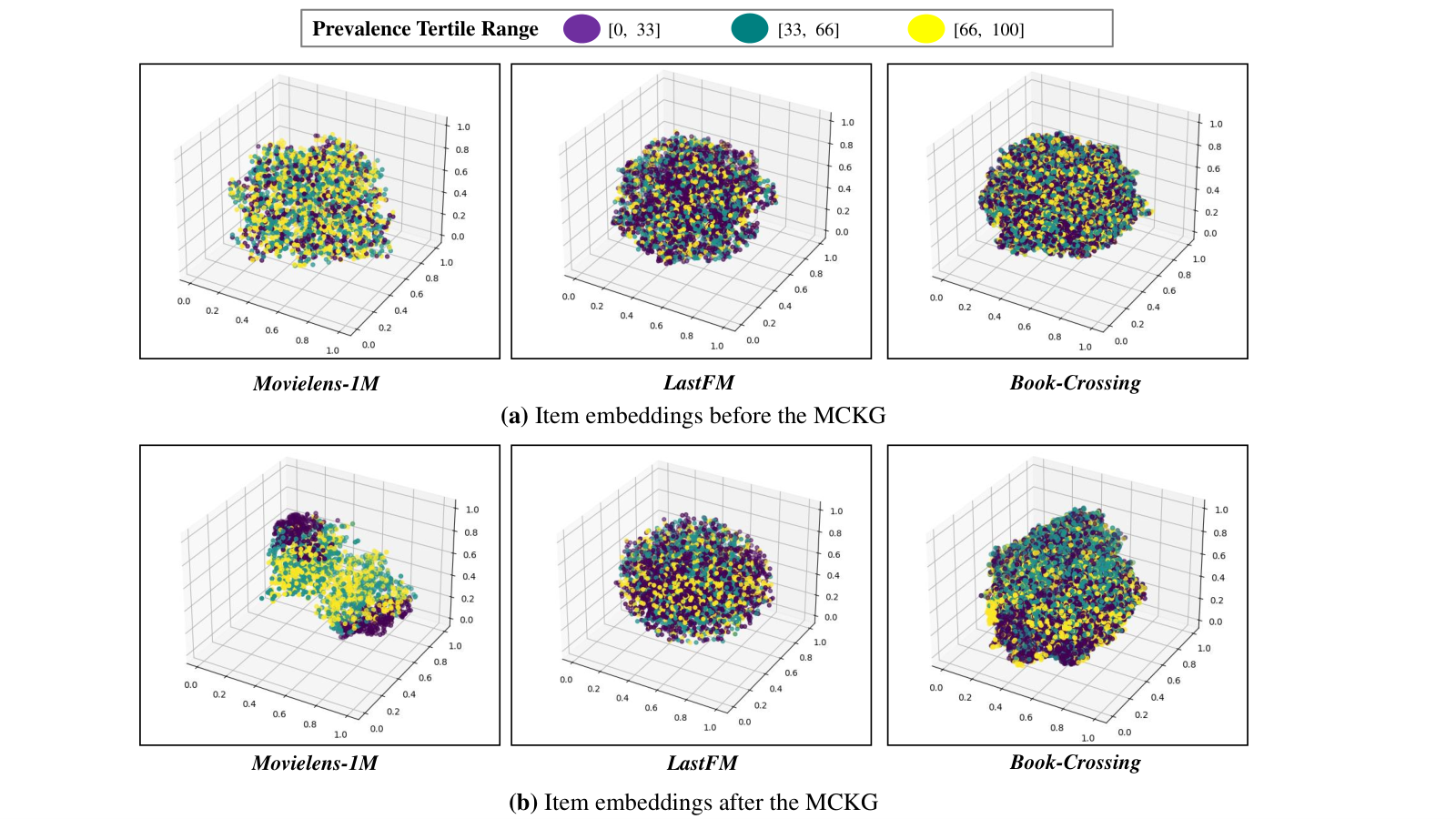
We used t-SNE to visualize the item embeddings as shown in Figure 4. Similar to HGCF (Sun et al. 2021), to better understand the influence of graph convolutions we depict item embeddings before and after the MCKG layers. Furthermore, the items are divided into three groups based on the prevalence of interactions, and we color each tertile independently.
Before performing MCKG, we can see that the three groups of item embeddings are evenly distributed in a sphere area. After feeding the three datasets to MCKG, we have the following observations:
- •
In Movielens-1M, we can clearly see that unpopular items (purple points) are pushed out at both ends, while the popular items (green and yellow points) are pulled in the middle region. This may be caused by the geometry-aware optimization strategy. Specifically, when the curvature is trainable, our model can distinguish items by popularity, whether in hyperbolic or spherical spaces.
- •
In LastFM, we hardly see a clear difference between the trained item embeddings and the original embeddings, but this may be more beneficial for the recommendation’s fairness. On the other hand, in Book-Crossing, we roughly see that the more popular items (green points) are distributed in the upper part of the sphere, and the unpopular items (purple points) are distributed in the lower part of the sphere.
4.5. Sparse Scene Study
Data sparsity is a serious problem in recommendation field, to study the performance of recommendation models in sparse circumstances, we change the training set ratio of Movielens-1M from 10% to 90%, the rest datasets as test set. From Table 7, compared with the ratio=90%, the HR@20 of each model decreases by 6.2%, 3.7%, 4.4%, 2.7%, 3.0%, 3.2% when ratio=10%.
With the change of ratio, HGCF fluctuates the most, which shows that compared to other KG-enhanced models, it is more susceptible to sparse data. This also confirms that using KG as auxiliary information is a effective strategy to improve recommendation performance in sparse scenarios. On the other hand, we found that the non-Euclidean methods (i.e., KBHP, LKGR and MCKG) perform more stable than the Euclidean methods (i.e., RippleNet and KGAT) in sparse scene. One possible reason is that due to the spatial characteristics of hyperbolic spaces, even in sparse scene, its ability to distinguish positive and negative items still be maintained.
| Model | Ratios of training set | %change. | ||||||||
|---|---|---|---|---|---|---|---|---|---|---|
| 10% | 20% | 30% | 40% | 50% | 60% | 70% | 80% | 90% | ||
| HGCF | 0.7183 | 0.7320 | 0.7346 | 0.7488 | 0.7503 | 0.7538 | 0.7631 | 0.7597 | 0.7633 | 6.2% |
| RippleNet | 0.7236 | 0.7256 | 0.7263 | 0.7279 | 0.7385 | 0.7492 | 0.7490 | 0.7504 | 0.7403 | 3.7% |
| KGAT | 0.7456 | 0.7648 | 0.7637 | 0.7646 | 0.7648 | 0.7729 | 0.7781 | 0.7786 | 0.7791 | 4.4% |
| KBHP | 0.7611 | 0.7729 | 0.7786 | 0.7865 | 0.7878 | 0.7810 | 0.7812 | 0.7817 | 0.7815 | 2.7% |
| LKGR | 0.7690 | 0.7697 | 0.7804 | 0.7806 | 0.7808 | 0.7910 | 0.7914 | 0.7905 | 0.7918 | 3.0% |
| MCKG | 0.7805 | 0.7809 | 0.7858 | 0.7962 | 0.7997 | 0.8023 | 0.8010 | 0.8008 | 0.8055 | 3.2% |
5. RELATED WORK
In this section, we review two relevant prior works: KG-enhanced recommendation methods and the hyperbolic representation learning.
5.1. KG-enhanced Recommendation Methods
Currently, KG-enhanced recommendation methods has gradually attracted the attention of researchers, here we divide them into embedding-based methods, path-based methods and GCN-based methods:
Embedding-based approaches typically use knowledge graph embedding (KGE) methods to endow knowledge graph for entity vectors, and further feed these vectors to recommendation module (Cai et al. 2018). For instance, to fully exploit the knowledge base, CKE (Zhang et al. 2016) considers three components to extract semantic features from the item’s structured content, textual content and visual content, respectively. Finally, CKE is formed to jointly learn the implicit vector of collaborative filtering and the semantics of items based on knowledge base. To dynamically adapt to user preference in real time, DKN (Wang et al. 2018b) adopts a sequential learning method, that is, the knowledge embedding learning module and the recommendation system module are independent of each other. It uses semantic information and knowledge information to represent news, and makes predictions based on user historical behavior and current candidate news.
Path-based approaches take into account various relationships between items and users in the knowledge network, which aims to offer accurate directions for recommendation tasks. Since the KG can construct heterogeneous information networks with user-item interactions, the conventional meta-path techniques can be applied to extracting heterogeneous information networks for recommendation. For instance, MCRec (Hu et al. 2018) learns representations of users, items and their interaction contexts, i.e., aggregated meta-paths. Specifically, MCRec uses a hierarchical neural network to model the meta-path context as a low-dimensional embedding, and enhances the three representations with a joint attention mechanism. Due to the introduction of meta-path-based context, this model not only has excellent performance, but also has a certain interpretability.
GCN-based methods typically employ iterative aggregation of the target node’s neighbors to fully mine the high-level information of KG. For instance, RippleNet (Wang et al. 2018a) takes the item clicked by the user as the origin, expands around like the water ripples, and constantly absorbs 1-hop and 2-hop neighbors to spread information. To automatically discover the semantic information of KG, KGCN (Wang et al. 2019c) samples from the neighborhood of each entity in KG as its receptive field, and then combines the neighborhood information with bias when computing the representation for a given entity. The receptive field can be further extended to multi-hops to model high-order information and capture users’ latent long-range interests. Similarly, KGAT (Wang et al. 2019a) updates a node’s embedding based on the embedding of its neighbors, and recursively performs this embedding propagation to capture high-order connectivity in linear time complexity. Additionally, an attention mechanism is employed to learn the weight of each neighbor during propagation.
5.2. Hyperbolic Representation Learning
Recently, Hyperbolic representation learning has taken an important role in RSs (Vinh Tran et al. 2020; Sun et al. 2021; Zhang et al. 2022a; Tai et al. 2021; Chen et al. 2022). HyperML (Vinh Tran et al. 2020) studies metric learning in hyperbolic space and its connection to CF. Furthermore, HGCF (Sun et al. 2021) proposes a hyperbolic GCN model for CF. To alleviate the power-law distribution in recommender systems, HICF (Yang et al. 2022) aims to improve the attention of tail items in hyperbolic spaces, which makes the pull and push process geometric-aware. On the other hand, to reveal the intent factors across geometric spaces, GDCF (Zhang et al. 2022a) learns geometric disentangled representations associated with user intentions and various geometries. It’s worth emphasizing that KBHP (Tai et al. 2021) and LKGR (Chen et al. 2022) are the most similar to our work. Both of them combine KG and hyperbolic representation learning. Different from existing methods that solely adopt a specific manifold, we introduce a unified manifold into KG-based methods to capture the structural information on global level and automatically learn the optimal curvature in the data.
6. CONCLUSION
In this work, we proposed a novel recommendation model named MCKG. Our key motivation is that existing non-euclidean recommendation methods have the following issues: 1) existing non-euclidean methods treat as a trainable parameter, but model parameters constraints depend on the changes of curvature. Once the curvature varies, the internal structure of manifold may be destroyed, and further unable to obtain high-quality embeddings; 2) Existing mix-curvature methods directly operate on various manifolds without considering the heterogeneity. To address the above problems, we introduce the unified space can interpolate smoothly between all geometries of constant curvature, apply multiple spaces fusion to obtain the high-quality embedding, and finally propose a geometry-aware optimization strategy compatible with hyperbolic and spherical spaces.
In future work, we will further study the mix-curvature method for other application scenarios, e.g., natural language processing (Liu et al. 2021; Choudhary et al. 2022), computer vision (Ermolov et al. 2022; Guo et al. 2022), such non-Euclidean modeling strategy learns embeddings of correlated data successfully with reduced distortion.
Acknowledgements.
This research work is supported by the National Key Research and Development Program of China under Grant No. 2021ZD0113602, the National Natural Science Foundation of China under Grant Nos. 62176014, 62276015, 62206266, the Fundamental Research Funds for the Central Universities.References
- (1)
- Bachmann et al. (2020) Gregor Bachmann, Gary Bécigneul, and Octavian Ganea. 2020. Constant curvature graph convolutional networks. In International Conference on Machine Learning. PMLR, 486–496.
- Cai et al. (2018) Hongyun Cai, Vincent W Zheng, and Kevin Chen-Chuan Chang. 2018. A comprehensive survey of graph embedding: Problems, techniques, and applications. IEEE Transactions on Knowledge and Data Engineering 30, 9 (2018), 1616–1637.
- Chami et al. (2019) Ines Chami, Zhitao Ying, Christopher Ré, and Jure Leskovec. 2019. Hyperbolic graph convolutional neural networks. Advances in neural information processing systems 32 (2019).
- Chen et al. (2020) Lei Chen, Le Wu, Richang Hong, Kun Zhang, and Meng Wang. 2020. Revisiting graph based collaborative filtering: A linear residual graph convolutional network approach. In Proceedings of the AAAI conference on artificial intelligence, Vol. 34. 27–34.
- Chen et al. (2022) Yankai Chen, Menglin Yang, Yingxue Zhang, Mengchen Zhao, Ziqiao Meng, Jianye Hao, and Irwin King. 2022. Modeling Scale-free Graphs with Hyperbolic Geometry for Knowledge-aware Recommendation. In Proceedings of the Fifteenth ACM International Conference on Web Search and Data Mining. 94–102.
- Choudhary et al. (2022) Nurendra Choudhary, Nikhil Rao, Sumeet Katariya, Karthik Subbian, and Chandan K Reddy. 2022. ANTHEM: Attentive hyperbolic entity model for product search. (2022).
- Ermolov et al. (2022) Aleksandr Ermolov, Leyla Mirvakhabova, Valentin Khrulkov, Nicu Sebe, and Ivan Oseledets. 2022. Hyperbolic vision transformers: Combining improvements in metric learning. In Proceedings of the IEEE/CVF Conference on Computer Vision and Pattern Recognition. 7409–7419.
- Grattarola et al. (2018) Daniele Grattarola, Daniele Zambon, Cesare Alippi, and Lorenzo Livi. 2018. Learning graph embeddings on constant-curvature manifolds for change detection in graph streams. stat 1050 (2018), 16.
- Gu et al. (2018) Albert Gu, Frederic Sala, Beliz Gunel, and Christopher Ré. 2018. Learning mixed-curvature representations in product spaces. In International Conference on Learning Representations.
- Gu et al. (2019) Albert Gu, Frederic Sala, Beliz Gunel, and Christopher Ré. 2019. Learning mixed-curvature representations in product spaces. In International Conference on Learning Representations.
- Guo et al. (2022) Yunhui Guo, Xudong Wang, Yubei Chen, and Stella X Yu. 2022. Clipped Hyperbolic Classifiers Are Super-Hyperbolic Classifiers. In Proceedings of the IEEE/CVF Conference on Computer Vision and Pattern Recognition. 11–20.
- Hamilton et al. (2017) William L Hamilton, Rex Ying, and Jure Leskovec. 2017. Inductive representation learning on large graphs. In Proceedings of the 31st International Conference on Neural Information Processing Systems. 1025–1035.
- Han et al. (2020) Zhen Han, Yunpu Ma, Peng Chen, and Volker Tresp. 2020. Dyernie: Dynamic evolution of riemannian manifold embeddings for temporal knowledge graph completion. arXiv preprint arXiv:2011.03984 (2020).
- Helgason (1978) Sigurdur Helgason. 1978. Differential geometry, Lie groups and symmetric spaces. Math. Surveys Monogr 83 (1978).
- Hu et al. (2018) Binbin Hu, Chuan Shi, Wayne Xin Zhao, and Philip S Yu. 2018. Leveraging meta-path based context for top-n recommendation with a neural co-attention model. In Proceedings of the 24th ACM SIGKDD international conference on knowledge discovery & data mining. 1531–1540.
- Huang et al. (2018) Jin Huang, Wayne Xin Zhao, Hongjian Dou, Ji-Rong Wen, and Edward Y Chang. 2018. Improving sequential recommendation with knowledge-enhanced memory networks. In The 41st International ACM SIGIR Conference on Research & Development in Information Retrieval. 505–514.
- Kochurov et al. ([n.d.]) Max Kochurov, Sergey Ivanov, and Eugeny Burnaev. [n.d.]. Are Hyperbolic Representations in Graphs Created Equal? ([n. d.]).
- Liu et al. (2019) Qi Liu, Maximilian Nickel, and Douwe Kiela. 2019. Hyperbolic graph neural networks. Advances in Neural Information Processing Systems 32 (2019).
- Liu et al. (2021) Zheng Liu, Xiaohan Li, Zeyu You, Tao Yang, Wei Fan, and Philip Yu. 2021. Medical triage chatbot diagnosis improvement via multi-relational hyperbolic graph neural network. In Proceedings of the 44th International ACM SIGIR Conference on Research and Development in Information Retrieval. 1965–1969.
- Niepert et al. (2016) Mathias Niepert, Mohamed Ahmed, and Konstantin Kutzkov. 2016. Learning convolutional neural networks for graphs. In International conference on machine learning. PMLR, 2014–2023.
- Peng et al. (2021) Wei Peng, Tuomas Varanka, Abdelrahman Mostafa, Henglin Shi, and Guoying Zhao. 2021. Hyperbolic deep neural networks: A survey. IEEE Transactions on Pattern Analysis and Machine Intelligence 14 (2021), 1–28.
- Qu et al. (2019) Yanru Qu, Ting Bai, Weinan Zhang, Jianyun Nie, and Jian Tang. 2019. An end-to-end neighborhood-based interaction model for knowledge-enhanced recommendation. In Proceedings of the 1st International Workshop on Deep Learning Practice for High-Dimensional Sparse Data. 1–9.
- Sala et al. (2018a) Frederic Sala, Chris De Sa, Albert Gu, and Christopher Ré. 2018a. Representation tradeoffs for hyperbolic embeddings. In International conference on machine learning. PMLR, 4460–4469.
- Sala et al. (2018b) Frederic Sala, Chris De Sa, Albert Gu, and Christopher Re. 2018b. Representation Tradeoffs for Hyperbolic Embeddings. In Proceedings of the 35th International Conference on Machine Learning (Proceedings of Machine Learning Research, Vol. 80), Jennifer Dy and Andreas Krause (Eds.). PMLR, 4460–4469.
- Skopek et al. (2019) Ondrej Skopek, Octavian-Eugen Ganea, and Gary Bécigneul. 2019. Mixed-curvature Variational Autoencoders. In International Conference on Learning Representations.
- Sun et al. (2021) Jianing Sun, Zhaoyue Cheng, Saba Zuberi, Felipe Pérez, and Maksims Volkovs. 2021. Hgcf: Hyperbolic graph convolution networks for collaborative filtering. In Proceedings of the Web Conference 2021. 593–601.
- Sun et al. (2020) Rui Sun, Xuezhi Cao, Yan Zhao, Junchen Wan, Kun Zhou, Fuzheng Zhang, Zhongyuan Wang, and Kai Zheng. 2020. Multi-modal knowledge graphs for recommender systems. In Proceedings of the 29th ACM International Conference on Information & Knowledge Management. 1405–1414.
- Tai et al. (2021) Chang-You Tai, Chien-Kun Huang, Liang-Ying Huang, and Lun-Wei Ku. 2021. Knowledge Based Hyperbolic Propagation. In Proceedings of the 44th International ACM SIGIR Conference on Research and Development in Information Retrieval. 1945–1949.
- Vinh Tran et al. (2020) Lucas Vinh Tran, Yi Tay, Shuai Zhang, Gao Cong, and Xiaoli Li. 2020. Hyperml: A boosting metric learning approach in hyperbolic space for recommender systems. In Proceedings of the 13th International Conference on Web Search and Data Mining. 609–617.
- Wang et al. (2018a) Hongwei Wang, Fuzheng Zhang, Jialin Wang, Miao Zhao, Wenjie Li, Xing Xie, and Minyi Guo. 2018a. Ripplenet: Propagating user preferences on the knowledge graph for recommender systems. In Proceedings of the 27th ACM International Conference on Information and Knowledge Management. 417–426.
- Wang et al. (2018b) Hongwei Wang, Fuzheng Zhang, Xing Xie, and Minyi Guo. 2018b. DKN: Deep knowledge-aware network for news recommendation. In Proceedings of the 2018 world wide web conference. 1835–1844.
- Wang et al. (2019c) Hongwei Wang, Miao Zhao, Xing Xie, Wenjie Li, and Minyi Guo. 2019c. Knowledge graph convolutional networks for recommender systems. In The world wide web conference. 3307–3313.
- Wang et al. (2021b) Shen Wang, Xiaokai Wei, Cicero Nogueira Nogueira dos Santos, Zhiguo Wang, Ramesh Nallapati, Andrew Arnold, Bing Xiang, Philip S Yu, and Isabel F Cruz. 2021b. Mixed-curvature multi-relational graph neural network for knowledge graph completion. In Proceedings of the Web Conference 2021. 1761–1771.
- Wang et al. (2019a) Xiang Wang, Xiangnan He, Yixin Cao, Meng Liu, and Tat-Seng Chua. 2019a. Kgat: Knowledge graph attention network for recommendation. In Proceedings of the 25th ACM SIGKDD International Conference on Knowledge Discovery & Data Mining. 950–958.
- Wang et al. (2019b) Xiang Wang, Xiangnan He, Meng Wang, Fuli Feng, and Tat-Seng Chua. 2019b. Neural graph collaborative filtering. In Proceedings of the 42nd international ACM SIGIR conference on Research and development in Information Retrieval. 165–174.
- Wang et al. (2021a) Xiang Wang, Tinglin Huang, Dingxian Wang, Yancheng Yuan, Zhenguang Liu, Xiangnan He, and Tat-Seng Chua. 2021a. Learning intents behind interactions with knowledge graph for recommendation. In Proceedings of the Web Conference 2021. 878–887.
- Yang et al. (2022) Menglin Yang, Zhihao Li, Min Zhou, Jiahong Liu, and Irwin King. 2022. Hicf: Hyperbolic informative collaborative filtering. In Proceedings of the 28th ACM SIGKDD Conference on Knowledge Discovery and Data Mining. 2212–2221.
- Zhang et al. (2016) Fuzheng Zhang, Nicholas Jing Yuan, Defu Lian, Xing Xie, and Wei-Ying Ma. 2016. Collaborative knowledge base embedding for recommender systems. In Proceedings of the 22nd ACM SIGKDD international conference on knowledge discovery and data mining. 353–362.
- Zhang et al. (2022a) Yiding Zhang, Chaozhuo Li, Xing Xie, Xiao Wang, Chuan Shi, Yuming Liu, Hao Sun, Liangjie Zhang, Weiwei Deng, and Qi Zhang. 2022a. Geometric Disentangled Collaborative Filtering. (2022).
- Zhang et al. (2022b) Yiding Zhang, Chaozhuo Li, Xing Xie, Xiao Wang, Chuan Shi, Yuming Liu, Hao Sun, Liangjie Zhang, Weiwei Deng, and Qi Zhang. 2022b. Geometric Disentangled Collaborative Filtering. In Proceedings of the 45th International ACM SIGIR Conference on Research and Development in Information Retrieval. 80–90.
