Simulator-Driven Deceptive Control
via Path Integral Approach
Abstract
We consider a setting where a supervisor delegates an agent to perform a certain control task, while the agent is incentivized to deviate from the given policy to achieve its own goal. In this work, we synthesize the optimal deceptive policies for an agent who attempts to hide its deviations from the supervisor’s policy. We study the deception problem in the continuous-state discrete-time stochastic dynamics setting and, using motivations from hypothesis testing theory, formulate a Kullback-Leibler control problem for the synthesis of deceptive policies. This problem can be solved using backward dynamic programming in principle, which suffers from the curse of dimensionality. However, under the assumption of deterministic state dynamics, we show that the optimal deceptive actions can be generated using path integral control. This allows the agent to numerically compute the deceptive actions via Monte Carlo simulations. Since Monte Carlo simulations can be efficiently parallelized, our approach allows the agent to generate deceptive control actions online. We show that the proposed simulation-driven control approach asymptotically converges to the optimal control distribution.
I Introduction
We consider a deception problem between a supervisor and an agent. The supervisor delegates an agent to perform a certain task and provides a reference policy to be followed in a stochastic environment. The agent, on the other hand, aims to achieve a different task and may deviate from the reference policy to accomplish its own task. The agent uses a deceptive policy to hide its deviations from the reference policy. In this work, we synthesize the optimal policies for such a deceptive agent.
We formulate the agent’s deception problem using motivations from hypothesis testing theory. We assume that the supervisor aims to detect whether the agent deviated from the reference policy by observing the state-action paths of the agent. On the flip side, the agent’s goal is to employ a deceptive policy that achieves the agent’s task and minimizes the detection rate of the supervisor. We design the agent’s deceptive policy that minimizes the Kullback-Leibler (KL) divergence from the reference policy while achieving the agent’s task. The use of KL divergence is motivated by the log-likelihood ratio test, which is the most powerful detection test for any given significance level [1]. Minimizing the KL divergence is equivalent to minimizing the expected log-likelihood ratio between distributions of the paths generated by the agent’s deceptive policy and the reference policy. We also note that due to the Bratagnolle-Huber inequality [2], for any statistical test employed by the supervisor, the sum of false positive and negative rates is lower bounded by a decreasing function of KL divergence between the agent’s policy and the reference policy. Consequently, minimizing the KL divergence is a proxy for minimizing the detection rate of the supervisor. We represent the agent’s task with a cost function and formulate the agent’s objective function as a weighted sum of the cost function and the KL divergence.
We assume that the agent’s environment follows discrete-time continuous-state dynamics. When the dynamics are linear, the supervisor’s (stochastic) policies are Gaussian, and the cost functions are quadratic, minimizing a weighted sum of the cost function, and the KL divergence leads to solving a linear quadratic regulator problem. However, we consider a broader setting with potentially non-linear state dynamics, non-quadratic cost functions, and non-Gaussian reference policies. In this case, the agent’s optimal deceptive policy does not necessarily admit a closed-form solution. While the agent’s problem can be solved using backward dynamic programming, this approach suffers from the curse of dimensionality.
We show that, under the assumption of deterministic state dynamics, the optimal deceptive actions can be generated using path integral control without explicitly synthesizing a policy. In detail, we propose a two-step randomized algorithm for simulator-driven control for deception. At each time step, the algorithm first creates forward Monte Carlo samples of system paths under the reference policy. Then, the algorithm uses a cost-proportional weighted sampling method to generate a control input at that time step. We show that the proposed approach asymptotically converges to the optimal action distribution. Since Monte Carlo simulations can be efficiently parallelized, our approach allows the agent to generate the optimal deceptive actions online.
The contributions of this paper are threefold: 1) The work studies a problem of deception under supervisory control for continuous-state discrete-time stochastic systems. Given a reference policy, we formalize the synthesis of an optimal deceptive policy as a KL control problem and solve it using backward dynamic programming. 2) For the deterministic state dynamics, we propose a path-integral-based solution methodology for simulator-driven control. We develop an algorithm based on Monte Carlo sampling to numerically compute the optimal deceptive actions online. Furthermore, we show that the proposed approach asymptotically converges to the optimal control distribution of the deceptive agent. 3) We present a numerical example to validate the derived simulator-driven control synthesis framework.
I-A Related Work
Deception naturally occurs in settings where two parties with conflicting objectives coexist. The example domains for deception include robotics [3, 4], supervisory control settings [5, 6], warfare [7], and cyber systems [8].
We formulate a deception problem motivated by hypothesis testing. This problem has been studied for fully observable Markov decision processes [5], partially observable Markov decision processes [6], and hidden Markov models [9]. Different from [5, 6, 9] that study discrete-state systems and directly solve an optimization problem for the synthesis of deceptive policies, we consider a nonlinear continuous-state system and provide a sampling-based solution for the synthesis of deceptive policies. In the security framework, [10, 11] study the detectability of an attacker in a stochastic control setting. Similar to our formulation, [10, 11] provide a KL divergence-based optimization problem. While we consider an agent whose goal is to optimize a different cost function from the supervisor, [10, 11] consider an attacker whose goal is to maximize the state estimation error of a controller.
KL divergence objective is also used in reinforcement learning [12, 13] to improve the learning performance and in KL control frameworks [14, 15] for the efficient computation of optimal policies. In [15], Ito et al. studied the KL control problem for nonlinear continuous-state space systems and characterized the optimal policies. Different from [15], we provide a randomized control algorithm based on path integral approach that converges to the optimal policy as the number of samples increases. Path integral control is a sampling-based algorithm employed to solve nonlinear stochastic optimal control problems numerically [16, 17, 18]. It allows the policy designer to compute the optimal control inputs online using Monte Carlo samples of system paths. The Monte Carlo simulations can be massively parallelized on GPUs, and thus the path integral approach is less susceptible to the curse of dimensionality [19].
I-B Notation
Let be a measurable space where is a Borel set and is a Borel -algebra. Suppose is a probability space. An -measurable random variable is a function whose probability distribution is defined by
represents a stochastic kernel on given . For simplicity, we write and as and . If and are probability distributions on then, the Kullback-Leibler (KL) divergence from to is defined as
if the Radon-Nikodym derivative exists, and otherwise. Throughout this paper, we use the natural logarithm. Let be the set of discrete time indices. A set of variables is denoted by and a Cartesian product of sets is denoted by . denotes the joint probability distribution of random variables on .
II Problem Formulation
We consider a setting in which a supervisor contracts an agent to perform a certain task. Suppose the agent operates in a stochastic environment and follows discrete-time continuous-state dynamics. Let the state transition law of the agent be denoted by , where the random variables and represent the state and the control input of the system at time . and are assumed to be Euclidean spaces with appropriate dimensions. Suppose a supervisor provides a (possibly stochastic) reference policy to the agent and expects the agent to follow the policy to accomplish a certain task. Here, is a stochastic kernel on given . The agent, on the other hand, aims to achieve a different task by minimizing the following cost function, which we henceforth call as path cost:
| (1) |
where for and represent the stage costs and the terminal cost, respectively. In order to minimize the path cost (1), the agent designs its policy (possibly stochastic) that may deviate from the reference policy . The agent also attempts to be stealthy to hide its deviations from the supervisor. While the agent executes its policy , suppose the supervisor observes its state-action paths , and uses a likelihood ratio test to detect whether the agent deviates from the reference policy. According to the Neyman–Pearson lemma, the likelihood-ratio test is optimal among all simple hypothesis tests for a given significance level [1]. In other words, we consider the worst-case scenario for the agent to be detected by the supervisor. Suppose the initial state of the agent is known. We denote the joint probability distribution of the state-action paths induced via the reference policy by
| (2) |
and the joint distribution induced via the agent’s policy by
| (3) |
Given a path that is randomly sampled under the agent’s policy, the supervisor computes the log-likelihood ratio (LLR)
| (4) |
The supervisor decides that the agent uses the reference policy if , and deviates from otherwise. Here is a constant chosen by the supervisor to obtain a specified significance level. An agent not wanting to be detected by the supervisor must minimize the LLR (4). However, since the agent’s trajectories are stochastic, the agent cannot directly minimize the LLR. We consequently consider that the agent’s goal is to minimize the expected LLR as follows:
| (5) |
where represents the expectation with respect to the probability distribution (II). Note that equation (5) also defines the Kullback-Leibler (KL) divergence between the agent’s distribution and the reference distribution . It can be shown that can be written as the stage-additive KL divergence between and as follows (see Appendix A):
| (6) |
Since the KL divergence is equivalent to the expected LLR (5), in this work, the KL divergence is used as a proxy for the measure of the agent’s deviations from the reference policy.
Minimizing the KL divergence is in fact equivalent to minimizing the detection rate of an attacker for an ergodic process as proved in [11]. While we do not consider an ergodic process, the use of KL divergence is still well-motivated by the Bretagnolle–Huber inequality [2]. Let be an arbitrary set of events that the supervisor will identify the agent as a deceptive agent, i.e., the agent followed . According to the Bretagnolle–Huber inequality, we have
| (7) |
where and denote the supervisor’s false positive and negative rates, respectively. The false positive rate is the probability that the supervisor will identify the well-intentioned agent as a deceptive agent, i.e., the agent’s policy is , but the supervisor thinks that the agent has followed . Similarly, the false negative rate is the probability that the supervisor will identify the deceptive agent as a well-intentioned agent. The Bretagnolle–Huber inequality (7) states that the sum of the supervisor’s false positive and negative rates is lower bounded by a decreasing function of the KL divergence between the distributions and . Therefore, an agent wanting to increase the supervisor’s false classification rate should minimize the KL divergence from to .
The goal of the agent is to design a deceptive policy that minimizes the expected path cost (1) while limiting the KL divergence (6). Using (1) and (6), we propose the following KL control problem for the synthesis of optimal deceptive policies for the agent:
Problem 1 (Synthesis of optimal deceptive policy).
| (8) | ||||
where is a positive weighting factor that balances the trade-off between the KL divergence and the path cost.
We explain the above KL control problem via the following example:
Example 1.
Consider a drone that is contracted by a supervisor to perform a surveillance task over an area. The supervisor prefers the drone to operate at high speeds (policy ) to improve the efficiency of the surveillance. The operator of the drone, the agent, on the other hand, prefers the drone to operate in a battery-saving, safe mode (policy ) to improve the longevity of the drone. The agent does not want to get detected by the supervisor and fired. Hence, the goal of the agent is to operate in a way that would balance the energy consumption () and the deviations from the behavior desired by the supervisor ().
III Synthesis of Optimal Deceptive Policies
In this section, we solve Problem 1 using backward dynamic programming and propose a policy synthesis algorithm based on path integral control.
III-A Backward Dynamic Programming
Notice that the cost function of Problem 1 possesses the time-additive Bellman structure and, therefore, can be solved by utilizing the principle of dynamic programming [20]. Define for each and , the value function:
| (9) | ||||
Notice that in (9), we used “inf” instead of “min” since we do not know if the infimum is attained. In the following theorem, we show that the infimum is indeed attained, and therefore, “inf” can be replaced by “min”.
Theorem 1.
The value function satisfies the following backward Bellman recursion with the terminal condition :
| (10) | ||||
and the minimizer of Problem 1 is given by
| (11) |
where
| (12) |
and is a Borel set belonging to the algebra .
Proof.
See Appendix C. ∎
Theorem 1 provides a recursive method to compute the value functions and optimal control distributions backward in time. As one can see, to perform the backward recursions (10) and (11), the function must be evaluated everywhere in the continuous domain . Therefore, in practice, an exact implementation of backward dynamic programming is computationally costly (unless the problem has a special structure, for example, linear state dynamics and quadratic costs). The computational cost grows quickly with the dimension of the state space of the system, which is referred to as the curse of dimensionality. In the next section (Section III-B), we show that under the assumption of the deterministic state transition law, the backward Bellman recursions can be linearized. This allows us to design a simulator-driven algorithm to compute optimal deceptive actions.
III-B Simulator-Driven Control via Path Integral Approach
In this section, we focus on a special case in which the agent’s dynamics are deterministic and propose a simulator-driven algorithm to compute the optimal deceptive actions via path integral control.
Assumption 1.
The state transition law is governed by a deterministic mapping as
| (13) |
that is, , where denotes the Dirac measure.
Remark 1.
Note that under Assumption 1, the agent can deviate from the reference policy only if it is stochastic. Otherwise, under any deviations from the reference policy, with a positive probability, the supervisor will be sure that the agent did not follow the reference policy. Therefore, in what follows, we consider the reference policy to be stochastic. The stochasticity of the reference policy could be to account for the unmodeled elements of the dynamics, to provide robustness, or to encourage exploration.
Remark 2.
Consider a special setting in which the state dynamics is linear in and , the reference policy distribution is Gaussian, and the cost functions and are quadratic in and . In such a setting, it can be shown that the optimal deceptive policy is also Gaussian and can be analytically computed by backward Riccati recursions similar to the standard Linear-Quadratic-Regular (LQR) problems. In this work, we consider a broader setting with possibly non-Gaussian reference distribution, non-linear state dynamics, and non-quadratic cost functions. In this case, the optimal deceptive policy might not be efficiently computed by solving backward recursions.
Now, we propose a path-integral-based solution approach for simulator-driven policy synthesis. Under assumption 1, we can rewrite (10) as
| (14) | ||||
We introduce the exponentiated value function as . Using , the Bellman recursion (14) can be linearized, and we get the following linear relationship between and :
| (15) | ||||
Note that in (15), by Assumption 1. Equation (15) is a linear backward recursion in . The linear solvability of the KL control problem is well-known in the literature (e.g., [14]). We remark that linearizability critically relies on Assumption 111 1 We remark that in prior works where the path integral method is used to solve stochastic control problems, a certain assumption (e.g. Eq. (9) in [16]) is made to reinterpret the original problem as a problem of designing the optimal randomized policy for a deterministic transition system.. Now, by recursive substitution, (15) can also be written as
Thus, by introducing the path cost function
we obtain
| (16) |
where the expectation is with respect to the probability measure (II). Equation (16) expresses the exponentiated value function as the expected path cost under the reference distribution. This suggests a path-integral-based approach to numerically compute . Suppose we generate a collection of independent samples of system paths starting from under the reference distribution . Since the reference distribution is known, a collection of such sample paths can be easily generated using a Monte Carlo simulation. If represents the path cost of the sample path , then by the strong law of large numbers [21] as , we get
| (17) |
Similarly, a collection of sample paths starting from under the reference distribution can be used to sample from the optimal distribution . Notice that the optimal deceptive policy (11) can be expressed in terms of as
| (18a) | ||||
| (18b) | ||||
| (18c) | ||||
The step (18a) follows from the definition of . In (18b), we used our assumption . Finally, (18c) is obtained by the recursive substitution of (18b), and represents a collection paths such that .
We use the above representation of to sample an action from it. Let be the exponentiated path cost of the sample path :
| (19) |
and . For each , we introduce a piecewise constant, monotonically non-decreasing function by
where denotes , i.e., the greatest integer less than or equal to . The function is represented in Figure 1.

;
For each sample path , compute the exponentiated path cost by (19).
Compute .
Generate a random variable according to .
Select a sample ID by .
Select a control input as .
Notice that the inverse of defines a mapping . To generate a sample approximately from the optimal distribution , we propose Algorithm 1. We first, generate a random variable according to . Then, we select a sample ID by . Finally, the control input adopted in the -th sample path at time step is selected as , i.e., . Theorem 2 proves that as the number of Monte Carlo samples tends to infinity, Algorithm 1 samples from the optimal distribution .
Theorem 2.
Let be a Borel set. Suppose for a given collection of sample paths , is computed by Algorithm 1 and the probability of is denoted by . Then, as
Proof.
See Appendix D ∎
We showed that under Assumption 1, the optimal deceptive policies can be synthesized using path integral control. Algorithm 1 allows the deceptive agent to numerically compute optimal actions via Monte Carlo simulations without explicitly synthesizing the policy. Since Monte Carlo simulations can be efficiently parallelized, the agent can generate the optimal control actions online.
IV Numerical Example

 (a) Paths under ,
(b) Paths under with ,
(a) Paths under ,
(b) Paths under with ,
 (c) Paths under with ,
(d) Paths under with ,
(c) Paths under with ,
(d) Paths under with ,
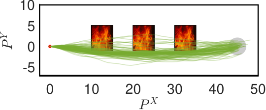
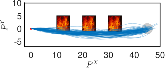
In this section, we validate the path-integral-based algorithm proposed to generate optimal deceptive control actions. The problem is illustrated in Figure 2. A supervisor wants an agent to start from the origin and reach a disk of radius centered at (shown in gray color) as fast as possible. The supervisor also expects the agent to inspect the region on the way. To encourage exploration and to provide robustness against unmodeled dynamics, the supervisor designs a randomized reference policy. The agent, on the other hand, wishes to avoid the regions on the way that are covered under fire, as shown in Figure 2. Let these regions be represented collectively by . Suppose the agent’s dynamics are modeled by a unicycle model as:
where , , and denote the position, speed, and the heading angle of the agent at time step , respectively. The control input consists of acceleration and angular speed . is the time discretization parameter used for discretizing the continuous-time unicycle model. For this simulation study, we set . Note that the agent’s dynamics is deterministic as per Assumption 1; however, the control input can be stochastic. Suppose the supervisor designs the reference policy as a Gaussian probability density with mean and covariance :
The mean is designed using a proportional controller as
where and are proportional gains and , are computed as
As mentioned before, the agent wishes to avoid the region . Suppose the cost function is designed as
where represents an indicator function that returns when the agent is inside the region and otherwise. For this simulation, we set
The agent chooses its action at each time step using Algorithm 1 where the number of samples is .
Suppose denotes the deceptive agent’s distribution generated by the sampling-based Algorithm 1. Figure 2 shows paths under the reference distribution R (Figure 2(a)) and the agent’s distribution for three values of (Figure 2(b) - 2(d)). A lower value of implies that the agent cares less about its deviation from the reference policy and more about avoiding the region . A higher value of implies the opposite. We also report , the percentage of paths that avoid . Under the reference distribution , only of the paths are safe. On the other hand, more paths are safe under the agent’s distribution , and as the value of reduces, increases.
Figure 3 shows the expected log-likelihood ratio (with one standard deviation) with respect to time for three values of . The expected LLR is computed as follows. Algorithm 1 selects a control input at time step , where is a sample ID obtained from step 1. From the construction of the algorithm, at each time step , the probability of choosing the control input under the agent’s distribution is , where and are computed by steps 1 and 1 of Algorithm 1. Whereas the probability of choosing the control input under the reference distribution is . Therefore, using (22), the expected LLR upto time can be approximately computed as
where is the number of paths generated by repeatedly running Algorithm 1. Note that since we assume the system dynamics to be deterministic (Assumption 1), once the control input is chosen at time step , the state is uniquely determined. Therefore, while computing the expected LLR, we only need to consider the probabilities of choosing the control input under policies and . Figure 3 shows that for a lower value of , the expected LLR is higher, i.e., more deviation of from .
V Conclusion
We presented a deception problem under supervisory control for continuous-state discrete-time stochastic systems. Using motivations from hypothesis testing theory, we formalized the synthesis of an optimal deceptive policy as a KL control problem and solved it using backward dynamic programming. Since the dynamic programming approach suffers from the curse of dimensionality, we proposed a simulator-driven algorithm to compute optimal deceptive actions via path integral control. The proposed approach allows the agent to numerically compute deceptive actions online via Monte Carlo sampling of system paths. We validated the proposed approach via a numerical example with a nonlinear system.
For future work, we plan to study the deception problem for continuous-time stochastic systems. We also plan to conduct the sample complexity analysis of the path integral approach to solve KL control problems.
-A Proof of Equation (6)
| (20a) | ||||
| (20b) | ||||
| (20c) | ||||
where, is a Borel set belonging to the algebra . The first equality (20a) follows from the definition (II), the second equality (20b) by the definition of the Radon-Nikodym derivative [21] and the last one (20c) from the definition (II). Using (20), we can write the Radon-Nikodym derivative as follows:
| (21) |
Using (21), we get the following:
| (22) | ||||
-B Legendre Duality
-C Proof of Theorem 1
By Bellman’s optimality principle, the value function satisfies the following recursive relationship:
| (23) |
where is defined by (12). Invoking the Legendre duality between the KL divergence and free energy (see Appendix B), it can be shown that there exists a minimizer of the right-hand side of (23), which can be written as
| (24) |
where is a Borel set belonging to the algebra . Using (24), the value of (23) can be computed as
| (25) |
Substituting (12) into (25), we obtain the recursive expression (10).
-D Proof of Theorem 2
References
- [1] T. M. Cover, Elements of information theory. John Wiley & Sons, 1999.
- [2] J. Bretagnolle and C. Huber, “Estimation des densités: risque minimax,” Séminaire de probabilités de Strasbourg, vol. 12, pp. 342–363, 1978.
- [3] J. Shim and R. C. Arkin, “A taxonomy of robot deception and its benefits in HRI,” in 2013 IEEE international conference on systems, man, and cybernetics. IEEE, 2013, pp. 2328–2335.
- [4] A. Dragan, R. Holladay, and S. Srinivasa, “Deceptive robot motion: synthesis, analysis and experiments,” Autonomous Robots, vol. 39, pp. 331–345, 2015.
- [5] M. O. Karabag, M. Ornik, and U. Topcu, “Deception in supervisory control,” IEEE Transactions on Automatic Control, vol. 67, no. 2, pp. 738–753, 2021.
- [6] ——, “Exploiting partial observability for optimal deception,” IEEE Transactions on Automatic Control, 2022.
- [7] M. Lloyd, The art of military deception. Pen and Sword, 2003.
- [8] C. Wang and Z. Lu, “Cyber deception: Overview and the road ahead,” IEEE Security & Privacy, vol. 16, no. 2, pp. 80–85, 2018.
- [9] C. Keroglou and C. N. Hadjicostis, “Probabilistic system opacity in discrete event systems,” Discrete Event Dynamic Systems, vol. 28, pp. 289–314, 2018.
- [10] E. Kung, S. Dey, and L. Shi, “The performance and limitations of epsilon-stealthy attacks on higher order systems,” IEEE Transactions on Automatic Control, vol. 62, no. 2, pp. 941–947, 2016.
- [11] C.-Z. Bai, F. Pasqualetti, and V. Gupta, “Data-injection attacks in stochastic control systems: Detectability and performance tradeoffs,” Automatica, vol. 82, pp. 251–260, 2017.
- [12] J. Schulman, S. Levine, P. Abbeel, M. Jordan, and P. Moritz, “Trust region policy optimization,” in International conference on machine learning. PMLR, 2015, pp. 1889–1897.
- [13] S. Filippi, O. Cappé, and A. Garivier, “Optimism in reinforcement learning and Kullback-Leibler divergence,” in 2010 48th Annual Allerton Conference on Communication, Control, and Computing (Allerton). IEEE, 2010, pp. 115–122.
- [14] E. Todorov, “Linearly-solvable Markov decision problems,” Advances in neural information processing systems, pp. 1369–1376, 2007.
- [15] K. Ito and K. Kashima, “Kullback–Leibler control for discrete-time nonlinear systems on continuous spaces,” SICE Journal of Control, Measurement, and System Integration, vol. 15, no. 2, pp. 119–129, 2022.
- [16] H. J. Kappen, “Path integrals and symmetry breaking for optimal control theory,” Journal of statistical mechanics: theory and experiment, vol. 2005, no. 11, p. P11011, 2005.
- [17] E. Theodorou, J. Buchli, and S. Schaal, “A generalized path integral control approach to reinforcement learning,” The Journal of Machine Learning Research, vol. 11, pp. 3137–3181, 2010.
- [18] G. Williams, P. Drews, B. Goldfain, J. M. Rehg, and E. A. Theodorou, “Aggressive driving with model predictive path integral control,” in 2016 IEEE International Conference on Robotics and Automation (ICRA). IEEE, 2016, pp. 1433–1440.
- [19] G. Williams, A. Aldrich, and E. A. Theodorou, “Model predictive path integral control: From theory to parallel computation,” Journal of Guidance, Control, and Dynamics, vol. 40, no. 2, pp. 344–357, 2017.
- [20] D. Bertsekas, Dynamic programming and optimal control: Volume I. Athena scientific, 2012, vol. 1.
- [21] R. Durrett, Probability: theory and examples. Cambridge university press, 2019, vol. 49.
- [22] M. Boué and P. Dupuis, “A variational representation for certain functionals of Brownian motion,” The Annals of Probability, vol. 26, no. 4, pp. 1641–1659, 1998.
- [23] E. A. Theodorou and E. Todorov, “Relative entropy and free energy dualities: Connections to path integral and KL control,” The 51st IEEE Conference on Decision and Control (CDC), pp. 1466–1473, 2012.
