A Bayesian approach for consistent reconstruction of inclusions
Abstract
This paper considers a Bayesian approach for inclusion detection in nonlinear inverse problems using two known and popular push-forward prior distributions: the star-shaped and level set prior distributions. We analyze the convergence of the corresponding posterior distributions in a small measurement noise limit. The methodology is general; it works for priors arising from any Hölder continuous transformation of Gaussian random fields and is applicable to a range of inverse problems. The level set and star-shaped prior distributions are examples of push-forward priors under Hölder continuous transformations that take advantage of the structure of inclusion detection problems. We show that the corresponding posterior mean converges to the ground truth in a proper probabilistic sense. Numerical tests on a two-dimensional quantitative photoacoustic tomography problem showcase the approach. The results highlight the convergence properties of the posterior distributions and the ability of the methodology to detect inclusions with sufficiently regular boundaries.
Keywords: inverse problems, Bayesian inference, inclusion detection, Gaussian prior, posterior consistency
1 Introduction
The Bayesian approach to inverse problems has in recent decades generated considerable interest due to its ability to incorporate prior knowledge and quantify uncertainty in solutions to inverse problems, see [1, 2]. A commonly recurring objective in inverse problems for imaging science is to recover inhomogeneities or inclusions, i.e. piecewise constant features, in a medium; applications range from cancer detection in medical imaging [3, 4] to defect detection in material science [5, 6]. In a Bayesian framework, this can be tackled by designing a prior distribution that favors images with these features.
An optimization-based approach can address this by parametrizing the relevant subset of the image space and minimizing a functional over the preimage of this parametrization, see for example [7]. This is visualized in Figure 1, where we consider the parametrization defined on a linear space and giving rise to the subset of the image space
where is a bounded and smooth domain in , and is a constant.
Such approaches benefit computationally from the fact that the set of images with inclusions, i.e. , form a low-dimensional subset of the image space . In the Bayesian framework, a related approach makes use of a push-forward distribution as the prior distribution, i.e. the distribution of a transformed random element of . This often leads to strong a priori assumptions, as the prior only gives mass to the range of the parametrization. More classical prior distributions including Laplace-type priors, see for example [8], and other heavy-tailed distributions often fail to take advantage of the low dimension of such images.
In this paper, we consider a Bayesian approach that captures this idea for two parametrizations used in detection of inclusions for nonlinear inverse problems: the star-shaped set and level set parametrizations. These parametrizations are studied rigorously in [9, 10, 11] and remain popular to Bayesian practitioners: we mention [1, 12, 13, 14, 15, 16] in the case of the star-shaped inclusions and [17, 18, 19, 20, 12, 21] for the level set inclusions, see also references therein.
The solution to the inverse problem in the Bayesian setting is the conditional distribution of the unknown given data, referred to as the posterior distribution. The posterior distribution has proved to be well-posed in the sense of [2] for such parametrizations.
This means that the posterior distribution continuously depends on the data in some metric for distributions.
This property implies, for example, that the posterior mean and variance are continuous with respect to the data, see [8]. However, such results give no guarantee as to where the posterior distribution puts its mass.
A more recent framework provided in [22] using ideas from [23], see also [24], gives tools to analyze the convergence of the posterior distribution for nonlinear inverse problems.
Such results, known as ‘posterior consistency’, address whether the sequence of posterior distributions arising from improving data (in a small noise or large sample size limit) gives mass approximating 1 to balls centered in the ground true parameter generating the data. Nonlinearity in the forward map and parametrization makes consistency results for Gaussian posterior distributions, as in [25], inapplicable. Currently, the setting of [22] and similar approaches require smoothness of the parameter of interest. A crucial condition is that the parameter set that is given most of the mass by the prior, has small ‘complexity’ in the sense of covering numbers, see [23, Theorem 2.1] or [24, Theorem 1.3.2]. Using Gaussian priors, this parameter set is typically a closed Sobolev or Hölder norm ball, see [24, Theorem 2.2.2] or [22]. However, such priors do not give sufficient mass to discontinuous parameters to conclude consistency. In this paper, we aim to address this, at least partially, by parametrizing the set of discontinuous parameters from a linear space of sufficiently smooth functions.
We aim to recover an element , which we call the image or the physical parameter, in a subset of for some continuous map .
We consider a nonlinear forward map mapping into a real separable Hilbert space with inner product and norm . We refer again to Figure 1 for an overview of this setup.
This setting allows us to make use of the framework provided in [22], but transfer the complexity condition from subsets of to subsets of , see Section 3.2. In the context of inclusion detection, this means we can detect inclusions with sufficiently smooth boundaries.
Our contributions can be summarized as follows:
- •
We present a posterior consistency result for the general setting mentioned above, when the parametrization satisfies mild conditions in regularity. We use the framework provided by [22] extending to Hölder continuous and push-forward priors. In particular, this gives an estimator, the posterior mean, which converges in probability to the true physical parameter in the small noise limit. Formally, this means there is an algorithm defined for noisy measurements depending on the noise level such that
in probability as . This statement will be made precise in Section 2. Furthermore, the rate of convergence is determined in part by the smoothness of elements in and the regularity of the parametrization.
- •
We show that two parametrizations for inclusion detection, a star-shaped set parametrization and a smoothened level set parametrization, satisfy the conditions for this setup. This verifies and quantifies the use of such parametrizations.
- •
We numerically verify the approach based on the two parametrizations in a small noise limit for a nonlinear PDE-based inverse problem using Markov chain Monte Carlo (MCMC) methods. We consider a two-dimensional quantitative photoacoustic (QPAT) problem of detecting an absorption coefficient. We derive a new stability estimate following [26, 27].
We note that the framework of [22] in e.g. [28] and [29] shows consistency for ‘regular link functions’ (defined in [30]), which are smooth and bijective. The archetypal example is or a smoothened version to ensure positivity of the physical parameter . As we shall see, injectivity and inverse continuity are not necessary for the proofs when we want to show consistency in . One novelty of our work is to show that this observation has relevance: we seek to recover the physical parameter instead of a non-physical parameter in that generated it. As we shall see, a natural parametrization for star-shaped inclusions is Hölder continuous from a suitable space to . The same holds true for a smoothened level set parametrization, which we will encounter in Section 4.2.
The structure of the paper can be summarized as follows. In Section 2, we recall a few key elements of the Bayesian framework in a ‘white noise’ model as outlined in [2] and [31, Section 7.4], including the notion of posterior consistency with a rate. In Section 3, we show that Hölder continuity of , some smoothness of elements in and conditional continuity of , suffice to show that the posterior mean
converges to the ground truth in as the noise goes to zero. Section 4 considers these conditions for the level set and star-shaped set parametrizations, which are well-known in the literature. In Section 5, we consider the two-dimensional quantitative photoacoustic tomography problem suited for piecewise constant parameter inference. Then, Section 6 gives background to our numerical tests and results that emulate the theoretical setting of Section 3. We present conclusive remarks in Section 7.
In the following, we let random variables be defined on a measure space . For a metric space the Borel -algebra is denoted by . If is a measurable map between the measure space and the measurable space , then denotes the push-forward measure defined by for all . We denote by the space of real-valued square integrable measurable functions from to . When is the Lesbegue measure on , we simply write . We call probability measures defined on Borel distributions.
2 The Bayesian approach to inverse problems
Bayesian inference in inverse problems centers around a posterior distribution. This is formulated by Bayes’ rule once a prior distribution in has been specified and the likelihood function has been determined by the measurement process. In this paper, we consider a ‘continuous’ model of indirect observations
| (1) |
for a continuous forward map , where the separable Hilbert space has an orthonormal basis . Here is ‘white noise’ in defined below in (4). We denote the noise level by for some and , which has this convenient form to study a countable sequence of posterior distributions in decreasing noise, i.e. for growing . When we write , it is understood that this depends on and . The rate is natural: if is a subspace of Hölder continuous functions on a bounded domain, this observation model is equivalent to observing discrete point evaluations of with added standard normal noise as , see [31] and [32, Section 1.2.3].
Given a Borel prior distribution on , the posterior distribution is proportional to the product of the likelihood and prior. Indeed, according to Bayes’ rule, if is finite-dimensional, the posterior distribution has a density (Radon-Nikodym derivative) of the form
where is a constant, see for example [8, 33]. This is well-defined for almost all under the marginal distribution of . The relevance of this object emerges, when evaluating it in a realization . Using inner product rules we can rewrite this as
| (2) |
where the contribution of is absorbed in the constant . The purpose of the following paragraphs is to argue that this formula remains valid, when is infinite-dimensional with the interpretation that is a Gaussian random variable defined by
| (3) |
where is a white noise process on satisfying and , see [32][Example 2.1.11]. To this end, let
| (4) |
which is convergent in in the mean square sense, see [8, Section 2.4], where is the Hilbert space , see also [31, Section 7.4], defined by
for and . Note is a Gaussian random element of , since it is the Karhunen-Loeve expansion of a mean zero Gaussian random element with covariance operator defined by , see [8].
Then is also a -valued Gaussian random element, since it is a translation of by an element in .
We denote the distributions of and in by and , respectively. We can think of as the data-generating distribution indexed by , the physical parameter generating the data, and , which controls the noise regime.
The likelihood function arises as the density (Radon-Nikodym derivative) of with respect to . This is a consequence of the Cameron-Martin theorem in the Hilbert space . The theorem gives the likelihood function as
here evaluated in , see [32][Proposition 6.1.5]. See also a derivation in [31, Section 7.4], for which it suffices that is continuous from (the standard Borel space) with the -topology into .
Then Bayes’ rule [33, p. 7] formulates a posterior distribution as a measure in as in the right-hand side of (2), well-defined for almost all . According to [33], this equals almost surely a Markov kernel, which we will call the posterior distribution and also denote it by . That is to say that is a measure for every and is measurable for every . In particular, is a -valued random variable.
Convergence in probability
In preparation for the subsequent section, we recall the notion of convergence in probability. Let be a decreasing sequence going to zero. For a fixed and a sequence of measurable functions we say that the sequence of random variables converges to in -probability with rate as if there exists a constant such that
| (5) |
as . We consider the following two cases, where we recall that both the posterior distribution and depend tacitly on .
- 1.
For a sequence of sets in , we could claim that
with rate as . That is, and . If this is the case for for some decreasing sequence going to zero and constant , we say that the posterior distribution contracts around or is consistent in at rate .
- 2.
Denote by the mean (‘posterior mean’) with respect to . This is defined in the sense of a Bochner integral,
which is well-defined by [34, Theorem 2], since for all
Then is an -valued random element by the definition of the Bochner integral and by the measurability of pointwise limits of measurable functions, see [35, Theorem 4.2.2]. We could claim that
with rate as . That is, and .
2.1 Posterior consistency
In this section we recall sufficient conditions posed in [22], see also [24], such that the posterior distribution in our specific setup is consistent. More specifically, we recall for which ground truths , forward models and prior distributions
| (6) |
as for some positive decreasing sequence going to zero. A consequence of this result, under additional assumptions on the prior, is that the posterior mean converges to in -probability, see [24, Theorem 2.3.2] or [33, Theorem 8.8],
| (7) |
with rate as . This is the case of (2) above. In the nonlinear inverse problem setting, posterior consistency in the sense of (6) follows from a two-step procedure with the use of conditional stability estimates.
- Step 1
The first step reduces convergence of from sets of the form
to sets of the form
Indeed, for specially chosen subsets which may depend on , assume we have the estimate
(8) for all and some . Then and hence
(9) where .
- Step 2
The second step involves showing that converges to in -probability as . This is posterior consistency on the ‘forward level’.
Combining Step 1 and Step 2, we find that converges to in -probability as . The ‘conditional’ stability estimate of the first step is of independent interest for many inverse problems in literature and usually requires an in-depth analysis of the inverse problem at hand. In this paper we treat first (8) as an assumption, see Condition 2. Although any modulus of continuity will do for the first step in this two-step procedure, for our concrete example in photoacoustic tomography we will show a Lipschitz stability estimate that holds for all , see Section 5. Our main motivation for including in the analysis is to keep the exposition generally applicable.
One of the contributions of [22, 24] is to address Step 2 for a random design regression observation model using the Theorem 2.1 in [23] and the equivalence between the distance (semi-metric)
and the Hellinger distance, see [24], of the data-generating distributions (corresponding to our ). Theorem 28 in [31], see also [32, Theorem 7.3.5], adapts the proof to the observation model (1), which is what we will use. One can see this second step as showing posterior consistency in at rate for the push-forward as in [36]. Below, we use the covering number for a semimetric , which denotes the minimum number of closed -balls of radius needed to cover , see Appendix A for a precise definition. Then the condition to complete Step 2 is as follows.
Condition A.
Let be a sequence of prior distributions in . Let be the forward model and the ground truth. Let satisfy for some . Suppose that,
- A.1
the prior gives enough mass to contracting balls .
(10) - A.2
there exist sets that are almost the support of in the sense that
(11) - A.3
and that there exists a constant such that
(12)
all for large enough.
Condition A.1 is a sufficient condition such that the denominator of the posterior distribution cannot decay too fast as . This is helpful when showing in -probability as . On the other hand Condition A.2 and A.3 are conditions that give control over the numerator in a sense that is made precise in the proof of Theorem 2.1 in [23] (or for example Theorem 28 in [31]). It is also a trade-off; the sets should be large enough such that they are almost the support of the prior, but small enough such that the covering number increases sufficiently slowly when . In the general case, Step 2 is completed by the following result proved in Appendix B.
Theorem 2.1.
2.2 Markov chain Monte Carlo
While Section 2.1 concludes in an abstract way the usefulness of the posterior distribution, in this section we briefly recall methods to approximate it. We consider MCMC methods that approximate (or other statistics) from averages of samples from a Markov chain that has the posterior distribution as its stationary distribution. Since the composition maps into continuously by assumption, given a prior distribution in , there exists a posterior distribution in of the form
| (14) |
Naturally, if , then by a change of variables
see for example [36, Theorem B.1], i.e. implies . This gives rise to the following ‘high-level’ algorithm: given a realization of ,
- 1.
choose and ,
- 2.
generate in using as initial condition with an MCMC method targeting , and
- 3.
return .
For our numerical examples, we use the preconditioned Crank-Nicolson (pCN) MCMC method, see [37]. This method uses only single evaluation of the log-likelihood function every iteration and is hence attractive for expensive PDE-based forward maps. It is well-defined when is a Hilbert space and possesses favorable theoretical properties, see [37, 38]. The idea to generate samples from by pushing forward samples also appears in certain reparametrizations of posterior distributions for the use of hyperparameters, see [39].
3 Posterior consistency using parametrizations
In this section, we follow [22, 24] in their approach to satisfy Condition A. In the case where for Gaussian and Lipschitz continuous, the approach is the same. We give a brief recap for the case where is Hölder continuous for the convenience of the reader. We tackle this by introducing three new conditions convenient for an inverse problem setting. We oppose this to Condition A, which is general and applicable in many statistical inference problems. As our base case, we assume , where is either the -dimensional torus or a bounded Lipschitz domain , and . We include here the torus in our considerations, since it is a numerically convenient setting. For more general parametrizations for inclusion detection, we shall need small deviations from this setting. However, these cases will take the same starting point of in Section 4. We begin by stating conditions on , and so that Condition A is satisfied. To do this, we introduce the following subset of .
We then require the following conditions of .
Condition 1 (On the parametrization ).
For any for some , let
| (15) |
for some constant and .
That is, we require at least conditional Hölder continuity of the parametrization map . The topology is not necessary for what follows and can be generalized to any , or -norm, . Similarly, we require conditional forward and inverse Hölder continuity of the forward map .
Condition 2 (On the forward map ).
For any , let
for some constants and . In addition, let
for some increasing function , which is continuous at zero with .
We have the following condition on the prior distributions we consider. They should be push-forward distributions of a scaled Gaussian prior distribution in .
Condition 3 (Prior ).
This gives the following structure
| (17) |
If one chooses for example a Matérn covariance, see [40], such that , then with , see Example 11.8 and Lemma 11.35 in [33] or [24, Theorem 6.2.3]. The scaling in (16) essentially updates the weight of the prior term to go slower to zero. Indeed, dividing through by the factor appearing in the data-misfit term, the prior term scales as . This term play the role of the ‘regularization parameter’ in [41]. Note that and , as is needed for the convergence of Tikhonov regularizers for example, see [41, Theorem 5.2]. The scaling (16) is also common in the consistency literature, see for example [22]. In our setting, it ensures that samples are with high probability in a totally bounded set , as was called for in Condition A.2 and A.3. We note for that is also a Gaussian measure on the separable Banach space endowed with the usual supremum norm . This is a consequence of a continuous Sobolev embedding and [42, Exercise 3.39].
Under Condition 1, 2 and 3, the lemmas in the subsequent sections ensure that Condition A is satisfied. Then we have the following theorem for posterior consistency at using the push-forward prior for a Gaussian distribution satisfying Condition 3.
Theorem 3.1.
Proof.
Note first that Lemma 3.4 shows that Condition A.1 is satisfied for some . Given , Lemma 3.2 states that we can choose such that Condition A.2 is satisfied and . For this choice of , Lemma 3.3 gives and such that Condition A.3 is satisfied. Then, by Theorem 2.1, there exists
with rate as . Then the wanted result is a consequence of (9). ∎
Posterior consistency with a rate as in the preceding theorem often leads to the convergence of related estimators with the same rate, see [33]. Here, we repeat an argument found in [24] to conclude that the posterior mean converges in -probability to as .
Corollary 1.
Under the assumptions of Theorem 3.1, the posterior mean in satisfies for some constant large enough
with rate as .
Proof.
3.1 Excess mass condition A.2
To motivate more precisely the scaling of the prior and the form of , we recall [22, Lemma 5.17]:
for all large enough and some fixed depending on . Then
| (19) |
Hence, charges with sufficient mass in relation to Condition A.2. However, we can consider a smaller set with the same property. Define
| (20) |
for .
Lemma 3.2.
3.2 Metric entropy condition A.3
Now we show that the sets on the form defined by (20) satisfy Condition A.3. This is straight-forward, when is Hölder continuous by Lemma A.1. We also recall that an upper bound on the covering number of Sobolev norm balls is well-known, see Lemma A.2.
Lemma 3.3.
3.3 Small ball condition A.1
In this section, we consider the strong assumption that . We refer the reader to [43] for a more general case where is only in the closure of in . However, this extension is not immediately compatible with the scaling (16). What follows in this section is based on the work [24]. We extend this to the case of Hölder continuous maps in a straight-forward manner. Below we need the scaled RKHS , see Condition 3, with norm
This is the RKHS associated with , see [42] or [32, Exercise 2.6.5].
Lemma 3.4.
Proof.
For large enough depending on and , we have by Condition 1 and 2,
| (24) | |||||
where and , and where we used the triangle inequality. Note also is a Gaussian measure in the separable Hilbert space . In addition, a closed norm ball in is a closed subset of and so is by a Sobolev embedding. Then we can apply the Gaussian correlation inequality [24, Theorem 6.2.2] to (24) so that
| (25) | |||||
To each of the factors in the right-hand side of (25) we apply [32, Corrollary 2.6.18] to the effect that for large
for using also that for large enough as follows from (19). The rest of the argument follows [28, Lemma 11] and uses [44, Theorem 1.2], see also Lemma A.2, and the continuous embedding to conclude
with and , which fits the choice (21) of . ∎
4 Parametrizations for inclusions
In this section, we make use of Theorem 3.1 for two specific parametrizations suited for inclusion detection: a star-shaped set parametrization and a level set parametrization. These are parametrizations on the form
| (26) |
for some Lebesgue measurable subsets of and constants for , which we denote collectively as . Since we consider parametrizations that map into , we will implicitly consider as the restriction of the right-hand side of (26) to . Note that recovering parameters on this form requires that we know a priori the parameter values . However, this could further be modelled into the prior. In the following, we construct as star-shaped sets and level sets.
4.1 Star-shaped set parametrization
We start by considering the parametrization for a single inclusion, i.e. . For simplicity of exposition, we consider the star-shaped sets in the plane, although it is straight-forward to generalize to higher dimensions. Let be a continuously differentiable -periodic function. We can think of as a function defined on the 1-dimensional torus . The boundary of the star-shaped set is a deformed unit circle: for a point in it takes for the form
Then we write
| (27) |
Let and define
| (28) |
We have the following conditional continuity result, where we for simplicity fix .
Lemma 4.1.
Let and with for . Then
where only depends on and .
Proof.
By the translation invariance of the Lebesgue measure, it is sufficient to bound the area of the symmetric difference for . We parameterize this planar set using , defined by
Note that implies by a continuous Sobolev embedding. We have
and the well-known change of variables formula,
where is the determinant of the Jacobian of the map . In the last line, we used that is locally Lipschitz as follows from the mean value theorem. ∎
Using the triangle inequality for the symmetric difference and the main result of [45], we would also have an estimate on the continuity of as defined on , i.e. on elements . We could then endow with a product prior which straight-forwardly satisfies Condition A.1. For simplicity we skip this extension. Instead, we gather the following conclusion that follows directly from Theorem 3.1 and Corollary 1.
Theorem 4.2.
Note that this is the rate of (18) with and . Clearly this convergence rate takes into account that a smooth star-shaped inclusion belongs to a low-dimensional subset of . One can think of this fast convergence rate (compared to Gaussian priors directly in ) as an expression of uncertainty reduction. Parameters on the form (28) carry some regularity. Indeed, using results in [46, 47] showing -Sobolev regularity for reduces to giving an upper bound of the area of the -tubular neighborhood of with respect to . This is provided by Steiner’s inequality, see [48], for , or more generally by Weyl’s tube formula, see [49], when . Then for .
Multiple inclusions
The case of multiple star-shaped inclusions is a straight-forward generalization using the triangle inequality. We consider for , the map
as in (26) with from in (27) with , , and where we set . We denote the direct product norm associated with the norm on , i.e.
We have the following continuity result.
Lemma 4.3.
Let with , for . For and we have
where only depends on , and .
Proof.
Parallel to the remark before Lemma 4.1, we mention that a statement similar to Lemma 4.3 holds true for a map defined on , if we in addition wish to infer . In preparation for the main result of this section let us change notation to suit the current setting. Let
| (30) |
We then endow with a (product) prior distribution of satisfying Condition 3:
| (31) |
for . The last equality is found in for example [50, Lemma 1.2]. For this prior, we have the following result, which is accounted for in Appendix C.
Theorem 4.4.
Note that this is the rate as of Theorem 4.2, i.e. the rate does not depend on the number of inclusions; this dependence appears in the constant .
4.2 Level set parametrization
In this section, we consider the level set parametrization of piecewise constant functions. The simplest case is to compose a given continuous function , for , i.e. , with the Heaviside function as
for . However, is not uniformly Hölder continuous on for any and hence does not satisfy Condition 1. Indeed, if is small near the set , small changes in can lead to big changes in . A lower bound on near this set suffices, as can be seen from the implicit function theorem, see Lemma C.1. This type of condition also appears in level set estimation of probability densities, see [51]. We illustrate this phenomenon by the following two-dimensional example.
Example 1.
Let the two-dimensional disc of radius . Take as the radially symmetric functions and for and . It is clear that for all , and that
as . However and so
The example is easy to extend to the more general case where the -norm is replaced with the -norm. Note also that for fixed , we have continuity of in this particular example. This fact generalizes to continuity of in functions that do not have critical points on . However, for the stronger Condition 1, it is not obvious how much mass Gaussian distributions give to functions whose gradient is lower bounded away from zero near . For this reason, we take a different approach. We define an approximation of for which Condition 1 is satisfied. This gives an approximate posterior distribution that contracts around . We shall see that if we take for some , then the approximation properties of to and a triangle inequality argument ensure we have consistency at . To this end, consider the continuous approximation of the Heaviside function
| (33) |
We want to note two straight-forward properties of :
| (34) |
and
| (35) |
We could even consider a smooth approximation for , as in [21], but this is not necessary for our case. To construct the continuous level set parametrization, take constants satisfying
for some . Given a continuous function define
and let be of the form (26). The corresponding approximate level set parametrization is then
| (36) |
where we define and for any . One can check that coincides with , when . Motivated by Example 1 and the property that stationary Gaussian random fields have almost surely no critical points on their level sets, we define the admissible level set functions as
where
Indeed, according to [52, Proposition 6.12], for each fixed we have
| (37) |
if and the covariance function associated with for is stationary. This is permitted since is a Gaussian process, see for example [53, Section 9.4]. Note also that it is known that since is a Borel set.
Lemma 4.5.
We have the following:
- (i)
If , then for and sufficiently small
- (ii)
For any ,
Proof.
For the following consistency result we let
| (39) |
We endow with a prior distribution that satisfies Condition 3 for such that the covariance kernel associated with the random field is stationary. For simplicity we assume for some in Condition 2. Then we have the following result proved in Appendix C.
Theorem 4.6.
Note that for weak inverse stability estimates, i.e. small, the obtained contraction rate approaches the usual rate (18).
5 Quantitative photoacoustic tomography problem
To test the convergence of the inclusion detection methods, we consider the following test problem in quantitative photoacoustic tomography, see [54, 27, 55]. The diffusion approximation in QPAT models light transport in a scattering medium according to an elliptic equation
| (42) |
where , , and are the optical diffusion and absorption parameters, respectively. The prescribed Dirichlet boundary condition defines the source of incoming radiation. It is well-known that (42) has a unique solution for each and for any nonzero source function of (42). Furthermore, we have the estimate
| (43) |
see for example [56, Chapter 6]. QPAT aims to reconstruct the optical parameters given the absorbed optical energy density map , which equals the product up to some proportionality constant that models the photoacoustic effect. In our simplified approach, we aim to invert the forward map
for a fixed . For smoothness and physical accuracy we assume
| (44) |
This setting allows a simple inverse stability estimate. First we have the following continuity result of .
Lemma 5.1.
Lemma 5.2.
Under the same assumptions of Lemma 5.1, there exists a constant such that
| (45) |
Proof.
See also [27, Theorem 3.1] and [26, Theorem 1.2]. Note solves
hence by elliptic regularity
| (46) |
Note by the trace theorem, see [58], for as in (44) there exists such that . By a Sobolev embedding for some depending on . Theorem 8.29 and the remark hereafter in [57] states that for some and that
where and . By the maximum principle [57, Theorem 8.1] we can collect the right-hand side to one constant . Now using the argument in [26, Lemma 12], which in return uses the Harnack inequality [57, Corollary 8.21] we conclude
| (47) |
where is a constant. Note
Combining this with (46) and (47) we have
∎
We note that satisfies Condition 2 for and . We also note that is a separable Hilbert space with an orthonormal basis consisting of the eigenfunctions of the Dirichlet Laplacian on . We conclude that this problem is suitable as a test problem, and that Theorem 4.4 and 4.6 apply. In Section 7 we discuss other suitable inverse problems.
6 Numerical results
We discuss our numerical tests in detecting inclusions for the QPAT tomography problem using the pCN algorithm of Section 2.2 and the parametrizations of Section 4. For simplicity we assume , the two-dimensional unit disk.
6.1 Observation model
As an approximation to the continuous observation model (1) for the numerical experiments we consider observing
| (48) |
where is an orthonormal basis of consisting of the eigenfunctions of the Dirichlet Laplacian on and is a suitable number. This observation is the sequence of coefficients of the projection of from (1) to the span of . As observing is equivalent to observing , see for example [28, Theorem 26]. Besides being a convenient approximation, this model has numerical relevance: there exists closed-form reconstruction formulas for in the first part of the photoacoustic problem, see [59, 60]. The likelihood function then takes the form
6.2 Approximation of the forward map
We approximate the forward map using the Galerkin finite element method (FEM) with piecewise linear basis functions over a triangular mesh of vertices and elements, see [54, 61]. When is discontinuous and continuous, we approximate it by
respectively. Here denotes the ’th element of the triangular mesh. That gives us two approximations of the forward map:
where is the FEM solution corresponding to and is the FEM solution corresponding to . For the smooth level set parametrization we use with nodes, while for the star-shaped set parametrization we use with elements.
We compute by solving the generalized eigenvalue problem arising from the FEM formulation of the Dirichlet eigenvalue problem with the Matlab function sptarn. Then is approximated using the mass matrix for with and .
6.3 Phantom, noise and data
The phantom we seek to recover consists of two inclusions:
where and are two star-shaped sets described by their boundaries:
where , see Figure 2. We compute and fix the optical diffusion parameter to following [61]. Here the scattering parameter equals smoothed with a Gaussian smoothing kernel of standard deviation using the Matlab function imgaussfilt.

We choose an illumination that is smooth and positive on defined by
where
and , , , , and . This is a superposition of three Gaussians, which illuminates the target well.

We simulate data as in (48) by computing on a fine mesh of elements and nodes. The corresponding projection can be seen in Figure 3. We choose such that the relative error
is in the range .
See Figure 3 for a realization of the white noise expansion (3) projected to the first orthonormal vectors and scaled so that it accounts for relative noise.
To estimate the approximation error, we compute the vector
for , , samples of the prior for the level set parametrization introduced in Section 6.4 below. We then compute , where is the trace of the sample covariance matrix of the vectors . For this choice minimizes the Kullback-Leibler distance to , see [37]. We compute in the same way using , and samples of the prior for the star-shaped set parametrization in Section 6.4.
6.4 Choice of prior
Star-shaped sets
To mirror the theoretical results of Theorem 4.4 for the phantom above, we consider a product distribution in . To this end, consider the usual real orthonormal basis of trigonometric functions , i.e. and . Consider the Karhunen-Loeve expansion
| (49) |
for with for , , and some constant . Note has a Laplace-type covariance operator, and (49) can be interpreted as the solution of a stochastic PDE [62]. Then almost surely, see [8]. According to Theorem I.23 in [33] and the definition of Sobolev spaces [63, Section 4.3], with equivalent norms, i.e. the prior distribution of (49) satisfies Condition 3. We take as the distribution of
| (50) |
for , and . In practice, we compute (49) truncated at . We do not rescale as the theoretical estimates demand. Instead, we handpick a suitable for each noise level. We use inpoly [64] to efficiently project to . We refer to Figure 4 for an example of a sample from this prior.
Level sets
For the level set parametrization, we consider a prior distribution in . Here is the torus corresponding to the square , where we choose , since it is recommended in for example [65] to embed in a larger domain to avoid boundary effects. Here, we consider the usual real orthonormal basis of trigonometric functions . We let
| (51) |
with for , and . Similar to above, the series exists almost surely as an element in , see [8]. The corresponding RKHS is , see [33]. We choose and consider the linear, bounded and surjective restriction , see [63, Section 4.4]. Then is a Gaussian random element in , and its RKHS is , see [32, Exercise 2.6.5]. We take as the distribution of
| (52) |
for and . In practice, we truncate (51) at . Also, we hand-pick and for each noise level. See Figure 4 for a sample of this prior.

6.5 Results
In this section we present the numerical results using the star-shaped and level set parametrizations in different noise regimes.
We use the algorithm described in Section 2.2 with the pCN method implemented with an adaptive stepsize targeting a 30% acceptance rate. The initial stepsize is denoted by . For an example of an implementation of this sampling method, we refer to the Python package CUQIpy, see [66]. For the star-shaped set parametrization, we choose the following prior and algorithm parameters in the order of the relative noise levels: , , , , and corresponding to inclusions of constant radius. In the same order, we choose for the level set parametrization the following prior and sampling parameters: , , , and .
For the star-shaped set parametrization, we obtain samples after a burn-in of , whereas for the level set parametrization, we take after samples as burn-in. We find this choice suitable, since the truncation in Section 6.4 leaves us with a higher dimensional sampling problem in the level set case. We base our posterior mean approximations on Monte Carlo estimates using equally spaced samples of the chain.
In Figure 5, we see the posterior mean of arising from the star-shaped set parametrization and observations with different noise levels. The posterior mean approximates the ground truth well for all noise levels. Note that
the posterior mean varies only slightly for each noise level and is approximately piecewise constant. This indicates little posterior variance.
This is due to a small noise level and the fast contraction rate that this inverse problem provides by virtue of (45).
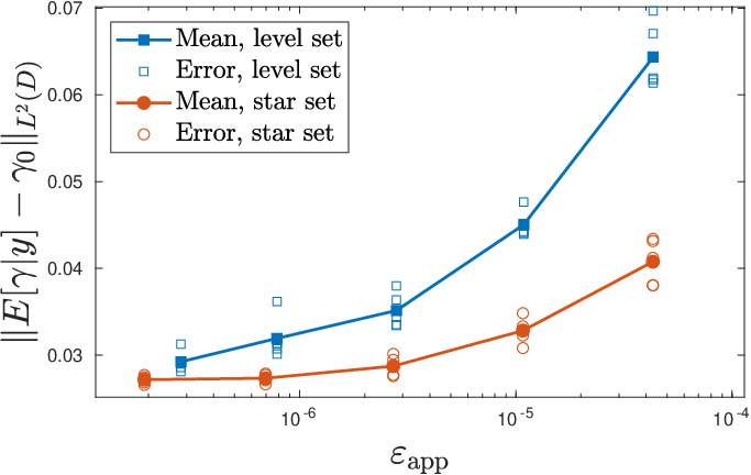
The estimates are not exact, but note that the exact data is not available due to projection and discretization. Taking large improves the data but also causes the likelihood function to attain larger values. This, in return, requires a smaller step size . This means there is a computational trade-off between and . Even for 16% relative noise, the reconstruction is fairly good, and the variance of the posterior samples is visibly larger. It is a strength of this method that it is robust for large noise levels. The mixing of the sample chains in the trace plots in Figure 7 indicates that the sampling algorithm is performing well. The convergence of the posterior mean is also evident in -distance as computed numerically, see Figure 8. This rate does not match the theoretical; but this is too much to expect for the observation (48), as this does not match the continuous observation (1) for which the rate is proved. Note we do not numerically scale the priors as the theoretical results require.

Figure 6 suggests that the posterior mean converges as the noise level goes to zero, as is also evident from its -loss in Figure 8. Note that the reconstructions are continuous, not only because we take an average, but also because we use a continuous level set parametrization. Here, the sampling is initialized at , since this guess captures some of the low frequency information of possible that can give rise to . We report that chains with small step-size and the natural starting guess often get stuck in local minima due to the number of levels in (52) and due to the fact that the pCN method does not require the gradient of either the parametrization or the forward map.
The sample diagnostics of Figure 7 indicate that sampling is harder for the level set parametrization compared to the star-shaped set parameterization. This is hard for at least two likely reasons: the first is due to the large number of coefficients , . This was also noted in [10]. The second likely reason is that is not injective for any . Therefore, the prior could be multi-modal, and this can lead to correlated samples in the Markov chain. Other work suggests that the pCN method shows an underwhelming performance when applied to a correlated and multi-modal posterior, see [67] which also provides a gradient-based remedy. The level set method has found success in optimization-based approaches, in for example [68], where a descent step is taken in each iteration of an iterative algorithm. A Bayesian maximum a posteriori approach [21] has also been shown to find success for a smoothened level set. We expect that using gradient information in gradient-based MCMC methods would improve the performance significantly. A benefit of the level set parametrization is that we do not need to know a priori the number of inclusions as in the case of the star-shaped set parametrization. One could also combine the two methods as in [12]. Note in Figure 8 that, for both parametrizations, the posterior mean is stable to different noise realizations. This mirrors the convergence in probability we expect from Theorem 4.4 and 4.6.


7 Conclusions
In this paper, we provide and investigate a Bayesian approach to consistent inclusion detection in nonlinear inverse problems. The posterior consistency analysis is performed under general conditions of Hölder continuity of the parametrization and conditional well-posedness of the inverse problem. Furthermore, it gives an explicit rate. We showcase the convergence of the posterior mean in a small noise limit for a photoacoustic problem, where we note that the star-shaped set parametrization outperforms the level set parametrization. We highlight that Theorem 4.2 and 4.6 hold for any forward map satisfying Condition 2 and can be applied to other parametrizations. A different parametrization could for example arise in the related problem of crack detection. Interesting future work includes applying the inclusion detection method to other inverse problems. Similar stability estimates to that of Lemma 5.2 exist for the mathematically closely related problems of determining the absorption coefficient in acousto-optic imaging and the permittivity in microwave imaging, see [26]. This is also the case for conductivity imaging in quantitative thermoacoustic tomography, where [69] employed complex geometrical optics solutions. For the Calderón problem in two dimensions, [70] provides a stability estimate that is permitted for the star-shaped set parametrization, see also the comments after Theorem 4.2 on the regularity of . There is a natural Hilbert space observation setting for the Calderón problem, see [28]. Also in three dimensions and higher, conditional stability for inclusion detection in the context of the Calderón problem has been considered and shown to be logarithmic at best [71]. The generalization to three dimensions and more complex phantoms is left for future work. An important direction in the numerical optimization of this approach is to consider gradient-based sampling methods.
Acknowledgments
The authors would like to thank Prof. Richard Nickl for many helpful discussions. The authors would also like to thank the Isaac Newton Institute for Mathematical Sciences, Cambridge, for support and hospitality during the program Rich and Nonlinear Tomography where work on this paper was undertaken, supported by EPSRC grant no EP/R014604/1. BMA, KK and AKR were supported by The Villum Foundation (grant no. 25893). TT was supported by the European Research Council (ERC) under the European Union’s Horizon 2020 research and innovation programme (grant agreement no. 101001417 - QUANTOM) and the Academy of Finland (Centre of Excellence in Inverse Modelling and Imaging project 353086 and the Flagship Program Photonics Research and Innovation grant 320166).
Appendix A Covering numbers
Consider a compact subset of a space endowed with a semimetric . The covering number denotes the minimum number of closed -balls with center and radius needed to cover , see for example [33, Appendix C] or [32, Section 4.3.7]. Then the metric entropy is . When is replaced by a norm, we mean the metric induced by the norm.
Lemma A.1.
Let and be two linear spaces endowed with semimetric and .
- (i)
If satisfies
for some and some , then for any we have
(53) - (ii)
For and ,
where is the product metric.
Proof.
We denote by and the ball in with center and radius and the ball in with center and radius , respectively. For any ,
Then it follows that
| (54) |
Let be a finite set in and be a finite set in such that
Take , then there exists such that and such that . Hence . It follows that
and hence the wanted property follows. ∎
Lemma A.2.
Let be a bounded Lipschitz domain in or the -dimensional torus and , then
where and .
Proof.
Corollary 4.3.38 and the remark hereafter in [32] states that the norm ball of the Sobolev space of radius satisfies for ,
| (55) |
If is the -dimensional torus, we identify with the corresponding periodic Sobolev space, which is a subset of , hence the wanted result follows. Now, if is a bounded Lipschitz domain in , we assume without loss of generality that . Indeed, if is not a subset of , we identify with for some by a scaling and update accordingly. Since is Lipschitz, we let be a continuous extension operator satisfying
see for example [72]. We denote the restriction , which is a contraction in supremum norm and the left-inverse of . Then and , and hence
| (56) | |||||
Lemma A.3.
With the notation defined in Section 3, we have for all
Appendix B On maximum likelihood composite testing
We denote by and the expectation with respect to and respectively.
Lemma B.1.
Suppose for a non-increasing function , some and all , we have
Then for every , there exist measurable functions such that
Proof.
To construct the measurable functions we use the maximum likelihood test, see [33, Lemma D.16] and the covering argument of [23, Theorem 7.1], see also [32, Theorem 7.1.4]. Choose a finite set of points in each shell
so that every is within distance of a point in . For , there are at most such points. For each , define the measurable function, , known as the maximum likelihood test,
where
By [33, Lemma D.16] we have
and
Now, set . This is also a measurable function, since a countable union of measurable sets is measurable. Then by the union bound
On the other hand, for any ,
For we get the wanted result. ∎
There are other ways to prove the existence of suitable measurable functions used in the proof of Theorem 2.1. We mention here the approximation argument of [28, Lemma 8] that requires smoothness properties of .
Proof of 2.1.
For the convenience of the reader, we provide what is a standard testing argument for our setting in Lemma B.1, see also [23, Theorem 7.1], implied by Condition A.3. Indeed, since the covering number decreases, when increasing the ‘radius’, we have for all ,
Given any , we set for large enough (depending also on , and by the following) and apply Lemma B.1: there exists measurable functions such that
In addition, choosing such that we note
Then Theorem 28 in [31] and modifications as in the proof of Theorem 1.3.2 in [24] give the claim. ∎
Appendix C Proofs of section 4
Proof of Theorem 4.4.
The proof relies on satisfying Condition A.1, A.2 and A.3 for the choice for
| (58) |
where is defined in (30). To satisfy Condition A.1 we follow Lemma 3.4 and note for and that
for some chosen sufficiently large. Then (31) together with the argument in Lemma 3.4 implies that Condition A.1 is satisfied. Note in (58) is the -product set of (20). Then repeated use of the standard set relation and the argument of Lemma 3.2 implies there exists such that
for any given , hence Condition A.2 is satisfied. Condition A.3 is satisfied as in Lemma 3.3 using Lemma A.1 . Then the result follows as in the proof of Theorem 3.1 and Corollary 1. ∎
Lemma C.1.
Let be defined as in (38) for , and some . Then for sufficiently small
Proof.
Note for and this is trivially satisfied. Next, the inverse function theorem implies that any point has a neighborhood that is a diffeomorphic image of a box
such that
(one should find the inverse of in a neighborhood of ). Note we have a parametrization of an intersection of with a small neighborhood of ,
for all . By the classical area formula, we have
since the continuous function (it is a polynomial of zero’th and first order derivatives of ), is integrated on a compact domain. Note is an open cover of for some finite set depending on and . Take such that . This exists since as defined on is a closed function, and hence there exists in a neighborhood of such that , see [73, Theorem 1.4.13]. Then,
This is true for any for which the estimate is only updated by a new constant. ∎
Proof of Theorem 4.6.
Let and for some , which we will choose later. For any , the triangle inequality gives
hence
| (59) | |||||
We shall consider the two factors of the right-hand side in separate parts below:
1) We check that Condition A.2, A.3, and A.1 are satisfied for the choice with
| (60) |
and to be chosen below. For A.2 it is clear from (37) that for each ,
As in the proof of Lemma 3.2 there exists such that Condition A.2 is satisfied, if is such that
| (61) |
for . This is satisfied when
| (62) |
so that . Condition A.3 follows as in the proof of Lemma A.1 with replaced with . Again it reduces to the covering number of the norm-ball in for which we need such that
as in (23). This is indeed satisfied by (62). For Condition A.1 we proceed as in the proof of Lemma 3.4 and use Lemma 4.5 to obtain
where . Continuing the argument and using (37), Condition A.1 is satisfied for some if again satisfies (61). By Theorem 2.1
as for some constant . It follows that
with rate , as as in Theorem 3.1.
2) For the second factor, note that and Lemma 4.5 (i) implies
Since is a strictly increasing function of (the rate becomes worse for larger ) and is strictly decreasing in , the optimal choice of satisfies , which is solved by
| (63) |
which also satisfies the condition on in (62), since . Inserting this back into (62) yields (41). Finally, take and and note by (59) that
in -probability as . Then the wanted result follows as in Corollary 1. ∎
References
- [1] Jari Kaipio and Erkki Somersalo. Statistical and computational inverse problems, volume 160 of Applied Mathematical Sciences. Springer-Verlag, New York, 2005.
- [2] A. M. Stuart. Inverse problems: a Bayesian perspective. Acta Numer., 19:451–559, 2010.
- [3] V Cherepenin, A Karpov, A Korjenevsky, V Kornienko, A Mazaletskaya, D Mazourov, and D Meister. A 3d electrical impedance tomography (EIT) system for breast cancer detection. Physiological Measurement, 22(1):9–18, feb 2001.
- [4] Minghua Xu and Lihong V. Wang. Photoacoustic imaging in biomedicine. Review of Scientific Instruments, 77(4):041101, 04 2006.
- [5] Milad Hallaji, Aku Seppänen, and Mohammad Pour-Ghaz. Electrical impedance tomography-based sensing skin for quantitative imaging of damage in concrete. Smart Materials and Structures, 23(8):085001, jun 2014.
- [6] Patrick Fuchs, Thorben Kröger, and Christoph S. Garbe. Defect detection in ct scans of cast aluminum parts: A machine vision perspective. Neurocomputing, 453:85–96, 2021.
- [7] Ashish Bora, Ajil Jalal, Eric Price, and Alexandros G. Dimakis. Compressed sensing using generative models. In Proceedings of the 34th International Conference on Machine Learning - Volume 70, ICML’17, page 537–546. JMLR.org, 2017.
- [8] Masoumeh Dashti and Andrew M. Stuart. The Bayesian approach to inverse problems. In Handbook of uncertainty quantification. Vol. 1, 2, 3, pages 311–428. Springer, Cham, 2017.
- [9] Tan Bui-Thanh and Omar Ghattas. An analysis of infinite dimensional bayesian inverse shape acoustic scattering and its numerical approximation. SIAM/ASA Journal on Uncertainty Quantification, 2(1):203–222, 2014.
- [10] Matthew M. Dunlop and Andrew M. Stuart. The Bayesian formulation of EIT: analysis and algorithms. Inverse Probl. Imaging, 10(4):1007–1036, 2016.
- [11] Marco A. Iglesias, Yulong Lu, and Andrew Stuart. A Bayesian level set method for geometric inverse problems. Interfaces Free Bound., 18(2):181–217, 2016.
- [12] Babak Maboudi Afkham, Yiqiu Dong, and Per Christian Hansen. Uncertainty quantification of inclusion boundaries in the context of X-ray tomography. SIAM/ASA J. Uncertain. Quantif., 11(1):31–61, 2023.
- [13] Ana Carpio, Sergei Iakunin, and Georg Stadler. Bayesian approach to inverse scattering with topological priors. Inverse Problems, 36(10):105001, 29, 2020.
- [14] Jeff Borggaard, Nathan E Glatt-Holtz, and Justin Krometis. A statistical framework for domain shape estimation in stokes flows. Inverse Problems, 39(8):085009, jun 2023.
- [15] Yunwen Yin, Weishi Yin, Pinchao Meng, and Hongyu Liu. The interior inverse scattering problem for a two-layered cavity using the Bayesian method. Inverse Probl. Imaging, 16(4):673–690, 2022.
- [16] Zhipeng Yang, Xinping Gui, Ju Ming, and Guanghui Hu. Bayesian approach to inverse time-harmonic acoustic scattering with phaseless far-field data. Inverse Problems, 36(6):065012, 30, 2020.
- [17] Matthew M. Dunlop, Marco A. Iglesias, and Andrew M. Stuart. Hierarchical Bayesian level set inversion. Stat. Comput., 27(6):1555–1584, 2017.
- [18] Neil K. Chada, Marco A. Iglesias, Lassi Roininen, and Andrew M. Stuart. Parameterizations for ensemble Kalman inversion. Inverse Problems, 34(5):055009, 31, 2018.
- [19] Jiangfeng Huang, Zhaoxing Li, and Bo Wang. A Bayesian level set method for the shape reconstruction of inverse scattering problems in elasticity. Comput. Math. Appl., 97:18–27, 2021.
- [20] Jiangfeng Huang, Zhiliang Deng, and Liwei Xu. A Bayesian level set method for an inverse medium scattering problem in acoustics. Inverse Probl. Imaging, 15(5):1077–1097, 2021.
- [21] William Reese, Arvind K Saibaba, and Jonghyun Lee. Bayesian level set approach for inverse problems with piecewise constant reconstructions. arXiv preprint arXiv:2111.15620, 2021.
- [22] François Monard, Richard Nickl, and Gabriel P. Paternain. Consistent inversion of noisy non-Abelian X-ray transforms. Comm. Pure Appl. Math., 74(5):1045–1099, 2021.
- [23] Subhashis Ghosal, Jayanta K. Ghosh, and Aad W. van der Vaart. Convergence rates of posterior distributions. The Annals of Statistics, 28(2):500 – 531, 2000.
- [24] Richard Nickl. Bayesian non-linear statistical inverse problems. Zurich Lectures in Advanced Mathematics. EMS Press, Berlin, 2023.
- [25] Sergios Agapiou, Stig Larsson, and Andrew M. Stuart. Posterior contraction rates for the Bayesian approach to linear ill-posed inverse problems. Stochastic Process. Appl., 123(10):3828–3860, 2013.
- [26] Mourad Choulli. Some stability inequalities for hybrid inverse problems. C. R. Math. Acad. Sci. Paris, 359:1251–1265, 2021.
- [27] Guillaume Bal, Kui Ren, Gunther Uhlmann, and Ting Zhou. Quantitative thermo-acoustics and related problems. Inverse Problems, 27(5):055007, 15, 2011.
- [28] Kweku Abraham and Richard Nickl. On statistical Calderón problems. Math. Stat. Learn., 2(2):165–216, 2019.
- [29] Matteo Giordano and Richard Nickl. Consistency of Bayesian inference with Gaussian process priors in an elliptic inverse problem. Inverse Problems, 36(8):085001, 35, 2020.
- [30] Richard Nickl, Sara van de Geer, and Sven Wang. Convergence rates for penalized least squares estimators in PDE constrained regression problems. SIAM/ASA J. Uncertain. Quantif., 8(1):374–413, 2020.
- [31] Richard Nickl. Bernstein–von Mises theorems for statistical inverse problems I: Schrödinger equation. J. Eur. Math. Soc. (JEMS), 22(8):2697–2750, 2020.
- [32] Evarist Giné and Richard Nickl. Mathematical foundations of infinite-dimensional statistical models. Cambridge Series in Statistical and Probabilistic Mathematics, [40]. Cambridge University Press, New York, 2016.
- [33] Subhashis Ghosal and Aad van der Vaart. Fundamentals of nonparametric Bayesian inference, volume 44 of Cambridge Series in Statistical and Probabilistic Mathematics. Cambridge University Press, Cambridge, 2017.
- [34] J. Diestel and J. J. Uhl, Jr. Vector measures. Mathematical Surveys, No. 15. American Mathematical Society, Providence, R.I., 1977. With a foreword by B. J. Pettis.
- [35] Richard M. Dudley. Real analysis and probability. The Wadsworth & Brooks/Cole Mathematics Series. Wadsworth & Brooks/Cole Advanced Books & Software, Pacific Grove, CA, 1989.
- [36] Sebastian J. Vollmer. Posterior consistency for Bayesian inverse problems through stability and regression results. Inverse Problems, 29(12):125011, 32, 2013.
- [37] S. L. Cotter, G. O. Roberts, A. M. Stuart, and D. White. MCMC methods for functions: modifying old algorithms to make them faster. Statist. Sci., 28(3):424–446, 2013.
- [38] Martin Hairer, Andrew M. Stuart, and Sebastian J. Vollmer. Spectral gaps for a Metropolis-Hastings algorithm in infinite dimensions. Ann. Appl. Probab., 24(6):2455–2490, 2014.
- [39] Matthew M. Dunlop, Tapio Helin, and Andrew M. Stuart. Hyperparameter estimation in Bayesian MAP estimation: parameterizations and consistency. SMAI J. Comput. Math., 6:69–100, 2020.
- [40] Lassi Roininen, Janne M. J. Huttunen, and Sari Lasanen. Whittle-Matérn priors for Bayesian statistical inversion with applications in electrical impedance tomography. Inverse Probl. Imaging, 8(2):561–586, 2014.
- [41] Heinz W. Engl, Martin Hanke, and Andreas Neubauer. Regularization of inverse problems, volume 375 of Mathematics and its Applications. Kluwer Academic Publishers Group, Dordrecht, 1996.
- [42] Martin Hairer. An introduction to stochastic pdes. arXiv preprint arXiv:0907.4178, 2009.
- [43] A. W. van der Vaart and J. H. van Zanten. Adaptive Bayesian estimation using a Gaussian random field with inverse gamma bandwidth. Ann. Statist., 37(5B):2655–2675, 2009.
- [44] Wenbo V. Li and Werner Linde. Approximation, metric entropy and small ball estimates for Gaussian measures. Ann. Probab., 27(3):1556–1578, 1999.
- [45] Daria Schymura. An upper bound on the volume of the symmetric difference of a body and a congruent copy. Adv. Geom., 14(2):287–298, 2014.
- [46] Winfried Sickel. Pointwise multipliers of Lizorkin-Triebel spaces. In The Maz’ya anniversary collection, Vol. 2 (Rostock, 1998), volume 110 of Oper. Theory Adv. Appl., pages 295–321. Birkhäuser, Basel, 1999.
- [47] Daniel Faraco and Keith M. Rogers. The Sobolev norm of characteristic functions with applications to the Calderón inverse problem. Q. J. Math., 64(1):133–147, 2013.
- [48] E Makai. Steiner type inequalities in plane geometry. Periodica Polytechnica Electrical Engineering (Archives), 3(4):345–355, 1959.
- [49] Alfred Gray. Tubes, volume 221 of Progress in Mathematics. Birkhäuser Verlag, Basel, second edition, 2004. With a preface by Vicente Miquel.
- [50] Olav Kallenberg. Foundations of modern probability, volume 99 of Probability Theory and Stochastic Modelling. Springer, Cham, [2021] ©2021. Third edition [of 1464694].
- [51] Guenther Walther. Granulometric smoothing. Ann. Statist., 25(6):2273–2299, 1997.
- [52] Jean-Marc Azaïs and Mario Wschebor. Level sets and extrema of random processes and fields. John Wiley & Sons, Inc., Hoboken, NJ, 2009.
- [53] Carl Edward Rasmussen and Christopher K. I. Williams. Gaussian processes for machine learning. Adaptive Computation and Machine Learning. MIT Press, Cambridge, MA, 2006.
- [54] T. Tarvainen, B. T. Cox, J. P. Kaipio, and S. R. Arridge. Reconstructing absorption and scattering distributions in quantitative photoacoustic tomography. Inverse Problems, 28(8):084009, 17, 2012.
- [55] Peter Kuchment. Mathematics of hybrid imaging: A brief review. In Irene Sabadini and Daniele C Struppa, editors, The Mathematical Legacy of Leon Ehrenpreis, pages 183–208, Milano, 2012. Springer Milan.
- [56] Lawrence C. Evans. Partial differential equations, volume 19 of Graduate Studies in Mathematics. American Mathematical Society, Providence, RI, 1998.
- [57] David Gilbarg and Neil S. Trudinger. Elliptic partial differential equations of second order, volume 224 of Grundlehren der mathematischen Wissenschaften [Fundamental Principles of Mathematical Sciences]. Springer-Verlag, Berlin, second edition, 1983.
- [58] J.-L. Lions and E. Magenes. Non-homogeneous boundary value problems and applications. Vol. I. Die Grundlehren der mathematischen Wissenschaften, Band 181. Springer-Verlag, New York-Heidelberg, 1972. Translated from the French by P. Kenneth.
- [59] Leonid A. Kunyansky. A series solution and a fast algorithm for the inversion of the spherical mean Radon transform. Inverse Problems, 23(6):S11–S20, 2007.
- [60] Mark Agranovsky and Peter Kuchment. Uniqueness of reconstruction and an inversion procedure for thermoacoustic and photoacoustic tomography with variable sound speed. Inverse Problems, 23(5):2089–2102, 2007.
- [61] Niko Hänninen, Aki Pulkkinen, and Tanja Tarvainen. Image reconstruction with reliability assessment in quantitative photoacoustic tomography. Journal of Imaging, 4(12), 2018.
- [62] Finn Lindgren, Hå vard Rue, and Johan Lindström. An explicit link between Gaussian fields and Gaussian Markov random fields: the stochastic partial differential equation approach. J. R. Stat. Soc. Ser. B Stat. Methodol., 73(4):423–498, 2011. With discussion and a reply by the authors.
- [63] Michael E. Taylor. Partial differential equations I. Basic theory, volume 115 of Applied Mathematical Sciences. Springer, New York, second edition, 2011.
- [64] Jeremy Kepner, Andreas Kipf, Darren Engwirda, Navin Vembar, Michael Jones, Lauren Milechin, Vijay Gadepally, Chris Hill, Tim Kraska, William Arcand, David Bestor, William Bergeron, Chansup Byun, Matthew Hubbell, Michael Houle, Andrew Kirby, Anna Klein, Julie Mullen, Andrew Prout, and Peter Michaleas. Fast mapping onto census blocks. In 2020 IEEE High Performance Extreme Computing Conference (HPEC), pages 1–8. IEEE, 2020.
- [65] U. Khristenko, L. Scarabosio, P. Swierczynski, E. Ullmann, and B. Wohlmuth. Analysis of boundary effects on PDE-based sampling of Whittle-Matérn random fields. SIAM/ASA J. Uncertain. Quantif., 7(3):948–974, 2019.
- [66] Nicolai Riis, Amal Alghamdi, Felipe Uribe, Silja Christensen, Babak Afkham, Per Christian Hansen, and Jakob Jorgensen. Cuqipy – part i: computational uncertainty quantification for inverse problems in python. arXiv preprint arXiv:2305.16949, 05 2023.
- [67] Tiangang Cui, Kody J. H. Law, and Youssef M. Marzouk. Dimension-independent likelihood-informed MCMC. J. Comput. Phys., 304:109–137, 2016.
- [68] Fadil Santosa. A level-set approach for inverse problems involving obstacles. ESAIM Contrôle Optim. Calc. Var., 1:17–33, 1995/96.
- [69] Ilker Kocyigit, Ru-Yu Lai, Lingyun Qiu, Yang Yang, and Ting Zhou. Applications of CGO solutions to coupled-physics inverse problems. Inverse Probl. Imaging, 11(2):277–304, 2017.
- [70] Albert Clop, Daniel Faraco, and Alberto Ruiz. Stability of Calderón’s inverse conductivity problem in the plane for discontinuous conductivities. Inverse Probl. Imaging, 4(1):49–91, 2010.
- [71] G. Alessandrini and M. Di Cristo. Stable determination of an inclusion by boundary measurements. SIAM J. Math. Anal., 37(1):200–217, 2005.
- [72] Ronald A. DeVore and Robert C. Sharpley. Besov spaces on domains in . Trans. Amer. Math. Soc., 335(2):843–864, 1993.
- [73] Ryszard Engelking. General topology, volume 6 of Sigma Series in Pure Mathematics. Heldermann Verlag, Berlin, second edition, 1989. Translated from the Polish by the author.