A unified perspective on Poincaré and Galilei relativity:
I. Special relativity
Abstract
A semantic adjustment to what physicists mean by the terms ‘special relativity’ and ‘general relativity’ is suggested, which prompts a conceptual shift to a more unified perspective on physics governed by the Poincaré group and physics governed by the Galilei group. After exploring the limits of a unified perspective available in the setting of 4-dimensional spacetime, a particular central extension of the Poincaré group—analogous to the Bargmann group that is a central extension of the Galilei group—is presented that deepens a unified perspective on Poincaré and Galilei physics in a 5-dimensional spacetime setting. The immediate focus of this paper is classical physics on affine 4-dimensional and 5-dimensional spacetimes (‘special relativity’ as redefined here), including the electrodynamics that gave rise to Poincaré physics in the first place; but the results here may suggest the existence of a ‘Galilei general relativity’ more extensive than generally known, to be pursued in the sequel.
keywords
keyword 1; keyword 2; keyword 3 (List three to ten pertinent keywords specific to the article; yet reasonably common within the subject discipline.)keywords
Relativity; Poincaré group; Galilei group; Bargmann group1 Introduction
In present common usage the terms ‘relativistic physics’ and ‘non-relativistic physics’ refer, at least roughly, to what might be called something else—perhaps ‘Poincaré physics’ and ‘Galilei physics’ respectively. These latter terms are intended here as shorthand for ‘physics governed by the Poincaré group’ and ‘physics governed by the Galilei group’. The motivation behind such a change in nomenclature, were it socially feasible, is that the essential innovation of what is commonly called ‘relativistic physics’ is the relativity of time, or more precisely, the relativity of simultaneity. In terms of space, so-called ‘non-relativistic physics’ is in an important sense just as relativistic as ‘relativistic physics’.
Absolute time—the notion that distinct events either do or do not occur at the same instant—is intuitive to ordinary human experience. This is manifest in the everyday expectation that if two observers carrying synchronized clocks each become aware of two distinct events, their clock readings will agree on whether the events occurred at the same time (after correction for finite travel time of light and sound from event to observer), regardless of the events’ separation in space or the relative motion of the observers. Einstein achieves the reconciliation of classical electromagnetism with classical mechanics only by abolishing this intuition; such is the cost of promoting the Maxwell equations, with their specification of the speed of light, to the status of physical law valid for all inertial observers.
True, a consequence of Einstein’s theory is that observers in relative motion disagree about intervals in both time and space (‘time dilation’ and ‘length contraction’ respectively), while in Newton’s world all observers agree on both durations measured by ideal clocks and the lengths of straight rulers, regardless of the motion of these clocks and rulers. This is presumably a major part of the rationale for nomenclature distinguishing between ‘relativistic’ and ‘non-relativistic’ theories. But the ‘relativistic’ phenomenon of length contraction is secondary or derivative, in the sense that in both Einstein’s and Newton’s worlds measurements of length must occur at a single instant, and therefore depend on a notion of simultaneity; while in Newton’s world no analogous specification—that measurements occur at the same place—is necessary in order to define measurement of time duration.
That measurements of lengths of objects depend upon a notion of simultaneity is a reminder that, unlike absolute time, absolute space is not as intuitive to ordinary human experience, at least upon reflection. (Apparently absolute space did seem obvious to Aristotle, and his later followers who dogmatically rejected Copernicus.) This is manifest in ready acceptance of the fact that if two observers carry triads of mutually orthogonal rulers in matching orientation, the answer to the question of whether two events occur in the ‘same place’ depends very much on both the time interval between the events and the relative motion of the observers. (Here ‘place’ means the 3-tuple of distances in each of the three dimensions of ordinary space between the events and the origins of the observers’ triads.) This translates into what is appropriately called the ‘Galilei relativity’ of the physics of the everyday human world, made persuasive—to the intelligent person of ordinary experience—by Galilei’s thought experiment about the inability to detect uniform motion of a ship based on observation of one’s immediate surroundings in a sealed cabin below decks (e.g. Penrose 2004).
That the relativity of time, rather than of space, is the crucial thing distinguishing Einstein circa 1905 from Newton is manifest in the celebrated equations relating the time intervals , and rectangular space intervals , between two events measured by two different observers and . Consider events sufficiently close in time and space that the two observers detect no linear acceleration (via spectral shifts) or rotation (via gyroscopes) in their own motion while they observe the two events Gourgoulhon 2013. Orient the observers’ -axes along the direction of the observers’ uniform relative motion, with moving with velocity as measured by , and align their - and -axes. In Newton’s world,
In Einstein’s world,
where is the speed of light and . Newton agrees with Einstein as . These transformations come from the homogeneous Galilei group on the one hand and the Lorentz group on the other; these are the linear parts of the Galilei and and Poincaré groups respectively, which include translations of the origin that cancel upon taking coordinate differences. These groups are appropriately named for consequential predecessors of the great synthesists Newton and Einstein.
Newton, while agreeing with Copernicus and Galilei, postulates absolute space in addition to absolute time, in order to formulate his theory given the mathematics of his era, and because of thought experiments about rotation (rotating pails of water, objects joined by a rope rotating about their center of mass) which raise questions not addressed by Galilei. Thus overturning both absolutes in a ‘relativistic’ theory comes to be associated with Einstein. And of course the overthrow of an ‘absolute space’ in the sense of a luminiferous aether as the medium in which light propagates also contributes to a sense that it is Einstein who relativizes space as well as time.
But it is apparent from the above transformations that the starkest difference is that time intervals are mixed into space intervals in both cases, while space intervals are mixed into time intervals only for Einstein. Thus the presence of ‘relativity’ in both cases—albeit space only in one case, and both space and time in the other—justifies more careful reference to, for instance, ‘Galilei relativity’ and ‘Poincaré relativity’, or ‘Galilei physics’ and ‘Poincaré physics’, instead of ‘non-relativistic physics’ and ‘relativistic physics’.
In the measurement of time and space intervals contemplated above, the stipulation of non-accelerated and non-rotating (i.e. ‘inertial’) observers points toward acknowledgment of another entrenched but unfortunate linguistic fossil: the use of the terms ‘special relativity’ and ‘general relativity’ to distinguish Einstein circa 1905 from Einstein circa 1915. Having freed the term ‘relativity’ from specific attachment to the world according to Einstein and recognizing its relevance to the world according to Newton, the terms ‘special relativity’ and ‘general relativity’ must be reconsidered as well. The main difference between Einstein circa 1905 and Einstein circa 1915, expressed in terms of the 4-dimensional ‘spacetime’ Minkowski introduces between them, is that the spacetime of Einstein circa 1905 is an affine space, which is flat, while the spacetime of Einstein circa 1915 is a more general pseudo-Riemann manifold whose curvature is determined by the energy and momentum of matter and radiation upon it (and indeed by the gravitational field itself, Einstein’s gravitation being a nonlinear theory). The latter is of course what enabled Einstein to accommodate gravity within a framework governed by the Poincaré group, with spectacular observational support from astrophysics and cosmology.
This distinction—between flat and curved spacetime, the latter with curvature determined by the presence of matter and radiation—is what ought to be meant by the terms ‘special relativity’ and ‘general relativity’, without regard for whether the physics is governed by the Poincaré group or the Galilei group. In this perspective the key difference is not between ‘relativistic physics’—whether ‘special’ or ‘general’—governed by the Poincaré group on the one hand, and ‘non-relativistic physics’ governed by the Galilei group on the other. Instead, what distinguishes ‘special relativity’ from ‘general relativity’ is whether the group in question—whether Poincaré, or Galilei—applies to spacetime globally, in which case it is an affine space; or only locally, in which case its curvature is determined by its energy and momentum content. The proper references, then, would be to ‘Poincaré special relativity’ and ‘Poincaré general relativity’, and to ‘Galilei special relativity’ and ‘Galilei general relativity’.
The purpose of this sequence of two papers is to demonstrate that these semantic shifts, unavoidably associated also with conceptual shifts, point toward a unified perspective on Poincaré and Galilei physics that may bear fruit in a Galilei general relativity more extensive than generally known, a possibility that has been briefly reported previously Cardall 2023. This first paper focuses on ‘special relativity’ as redefined above, that is, physics on spacetimes that are affine spaces (and therefore flat manifolds)—both ‘Poincaré special relativity’ and ‘Galilei special relativity’. The physics to be addressed in this first paper includes the motion of material particles and electrodynamics, the latter being tied historically both to the emergence of the Poincaré group and to the very notion of spacetime. The second paper will focus on ‘general relativity’ as redefined above, that is, physics on spacetimes that are curved manifolds—both ‘Poincaré general relativity’ and ‘Galilei general relativity’. The physics to be addressed in the second paper includes the motion of material continua and gravitation, the latter being tied historically to the reconciliation of the Poincaré group with gravitational physics by encoding the latter in the curvature of spacetime. Only classical (which here means ‘non-quantum’, not ‘non-Poincaré’) physics will be considered.
A conceptual roadmap to the spacetimes addressed by (or at least mentioned in) this sequence of two papers is given in Fig. 1. The prefix indicates a 5-dimensional Bargmann extension of a traditional 4-dimensional spacetime. The affine spacetimes and , and their affine Bargmann extensions and , are the primary focus of this paper. Curved spacetimes will be addressed in the sequel, with a primary goal of developing a conjectured ‘Galilei general relativity’ more extensive than generally known, whose spacetime is labeled labeled .
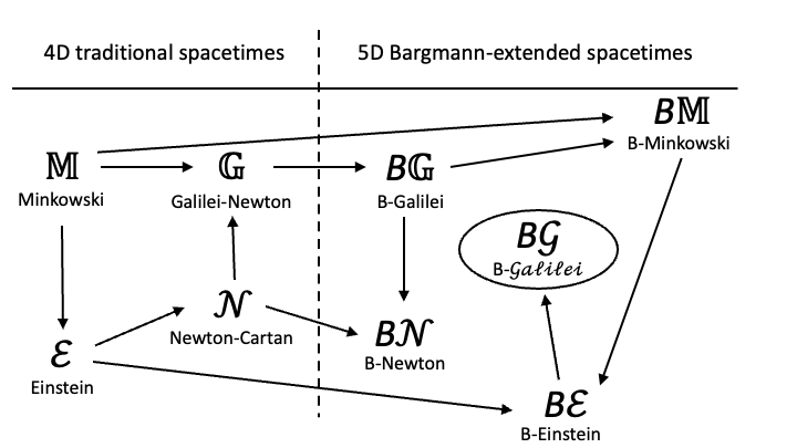
In historical terms, and continuing to refer to Fig. 1, the notion of spacetime begins in earnest with Minkowski’s 4-dimensional geometric reformulation of physics according to Poincaré and Einstein circa 1905 (traditionally known as ‘special relativity’) on a 4-dimensional affine space . Einstein circa 1915 subsequently generalizes to physics on a 4-dimensional curved spacetime (traditionally known as ‘general relativity’). With hindsight, the spacetime perspective of Minkowski and Einstein is backported to the physics of Galilei and Newton in the 1920s with the work of Weyl Weyl 1922 and Cartan Cartan 1923; Cartan 1924; Cartan 1986; examples of subsequent expositions include those of Toupin and Truesdell Toupin 1957; Truesdell and Toupin 1960, Havas Havas 1964, Trautmann Trautman 1965; Trautman 1966, and Küntzle Künzle 1972. Newton gravity is accommodated in the spacetime curvature of the resulting Newton-Cartan spacetime , though the 3-space leaves of the foliation according to absolute time are flat (traditional 3-dimensional Euclid position space); moreover the geometry is not pseudo-Riemann (there is no non-degenerate spacetime metric), and the field equations with mass density as a source are somewhat ad-hoc in comparison with the tight theoretical structure of physics on .
The flat (affine space) version of , Galilei-Newton spacetime , can be understood as being in effect augmented to a fifth dimension due to quantum mechanical considerations originally articulated by Bargmann Bargmann 1954 and discussed also for instance by Lévy-Leblond Lévy-Leblond 1971; Lévy-Leblond 1974; Lévy-Leblond 1976 and by Omote et al. Omote et al. 1989. It is subsequently recognized, for example by Souriau Souriau 1970; Souriau 1997, by Duval et al. Duval et al. 1985; Künzle and Duval 1986; Duval et al. 1991, by de Montigny et al. de Montigny et al. 2003a; de Montigny et al. 2003b, and by de Saxcé and Vallée de Saxcé and Vallée 2012; de Saxcé and Vallée 2016; de Saxcé 2017, that the extended affine and curved Bargmann spacetimes and are useful for classical Galilei physics as well. One bright spot is that these extended spacetimes are now pseudo-Riemann spaces (there is now a non-degenerate spacetime metric, see e.g. Pinski 1968; Duval et al. 1985; Künzle and Duval 1986; Omote et al. 1989; de Montigny et al. 2003a; de Montigny et al. 2003b; de Saxcé and Vallée 2016; de Saxcé 2017), though the comparatively ad-hoc nature of the field equations encoding Newton gravity remains somewhat unsatisfying.
The first few sections of this paper treat Poincaré and Galilei relativity in as unified a manner as possible from within a 4-dimensional perspective. Minkowski spacetime and Galilei-Newton spacetime are discussed in Sec. 2, including in particular their foliation into position space 3-slices and corresponding 1+3 (time/space) tensor decompositions. Spacetime treatments of a material particle and of the electromagnetic field on and follow in Secs. 3 and 4.
Subsequent sections of this paper illustrate the more unified perspective on Poincaré and Galilei relativity made possible by a 5-dimensional spacetime setting.
A fundamental difference between Poincaré and Galilei physics is the unification of inertia and total energy in the Poincaré case, in contrast to the invariant nature of inertia and its strict separation from kinetic energy in the Galilei case. Consideration of the inertia-momentum 4-vector (4-velocity of a material particle multiplied by its rest mass) shows that the Poincaré and Galilei groups naturally address the transformations of inertia and 3-momentum. In the Poincaré case the total energy goes along for the ride thanks to its equivalence to inertia, but in the Galilei case kinetic energy is left out in the cold: strictly separated from inertia, kinetic energy is not addressed by Galilei transformations. The traditional Bargmann group—called in this paper the Bargmann-Galilei or B-Galilei group, and associated with an extended 5-dimensional spacetime —is a central extension of the Galilei group that includes the transformation of kinetic energy, enabling a proper understanding of Galilei physics in quantum mechanics Bargmann 1954; Lévy-Leblond 1971; Lévy-Leblond 1974; Lévy-Leblond 1976 and a spacetime tensor treatment of material continua that includes kinetic energy and internal energy de Saxcé and Vallée 2012; de Saxcé and Vallée 2016; de Saxcé 2017.
What does not seem widely known or appreciated is the existence of what are called here the Bargmann-Poincaré (or B-Poincaré) group, and its linear part, the Bargmann-Lorentz (or B-Lorentz) group, and their association with a 5-dimensional spacetime called here Bargmann-Minkowski or B-Minkowski spacetime .11 1 These extended Lorentz/Poincaré transformations are noticed—perhaps uniquely, and almost as an afterthought—by Omote et al. Omote et al. 1989, a reference unearthed after publication of Cardall 2023. Because it already transforms total energy, a central extension of the Lorentz and Poincaré groups is in some sense not needed; but it is allowed, and provides for a more unified perspective on Poincaré and Galilei physics. Unlike the relationship between the 4-dimensional spacetimes and , these extended Poincaré structures associated with limit smoothly to their counterparts associated with as .22 2 Duval and Künzle and collaborators Duval et al. 1985; Künzle and Duval 1986 note that Poincaré and Galilei physics both can be addressed from a common 5-dimensional setting; but unlike Omote et al. Omote et al. 1989 and the present work, do not seem to have noticed and explicitly specified the B-Poincaré and B-Lorentz transformations and the even more unified perspective on Poincaré and Galilei physics they afford. These matters are discussed in Sec. 5, including in particular the foliation of and into position space 3-planes and corresponding 1+3+1 (time/space/action) tensor decompositions necessary to make contact with observations. Treatments of a material particle and of the electromagnetic field on and follow in Secs. 6 and 7. Reasons supporting a conjectured ‘Galilei general relativity’ more extensive than generally known, whose spacetime is labeled , are given in Sec. 8.
Affine spaces and linear tensors are briefly reviewed in the Appendix. In order to establish notation and the geometric perspective employed here, thorough familiarity with the Appendix is recommended before proceeding to Sec. 2. In any case, two grave warnings on notation deserve emphasis. First, in this work the infix dot operator () between two tensors will never denote a scalar product, if such exists, between two vectors; such will always be expressed explicitly in terms of the metric tensor defining the scalar product. Here the dot operator will instead denote only tensor evaluation, or contraction, via an obvious ‘pairing between lower and upper indices’. Second, index notation will be used sparingly, so that when a tensor or tensor field is introduced, careful attention should be paid to its type.
2 The affine spacetimes and
Minkowski spacetime and Galilei-Newton spacetime are affine spaces of dimension 4 whose points are called ‘events’. These spacetimes are endowed with additional structure (related to causality) on their respective underlying vector spaces and whose preservation requires restriction to particular subgroups of . For the required subgroup of is the Lorentz group ; for it is the homogeneous Galilei group . These are the linear (that is, homogeneous) parts of the Poincaré group (or inhomogeneous Lorentz group) and Galilei group respectively; the latter are the subgroups of comprising the symmetries of and respectively, which add translations to the Lorentz group and to the homogeneous Galilei group .
2.1 Minkowski spacetime
The causal structure on to be preserved is the null cone, embodied in a metric tensor of , a symmetric and non-degenerate bilinear form that defines a scalar product on . The metric is such that for any vectors , there exists a basis of such that
| (1) |
where the scalar is the speed of light, and and define the components and of and respectively. Note the summation convention, with Greek indices taking values in , with letters near the beginning of the Greek alphabet preferred for dummy indices, and letters from later in the alphabet preferred for free indices. Let be the dual space of and the basis dual to . With respect to this dual basis, it is apparent from Eq. (1) that
| (2) |
The null cone of is the set of all vectors such that .
The particular basis considered above is not the only one for which the scalar product takes not only the value, but the algebraic form exhibited in Eq. (1). Let be the Minkowski matrix
| (3) |
and the matrix
| (4) |
collecting the components of . Note that latin indices take values in , and that letters near the middle of the alphabet are preferred for free indices; letters near the beginning of the alphabet will be preferred for dummy indices. With respect to the particular basis considered above, it follows from Eq. (2) that the matrix representing is the Minkowski matrix:
| (5) |
Let and be the -column representations of with respect to the considered basis (see the Appendix). Then Eq. (1) is expressed by the matrix equation
| (6) |
Lorentz transformations are the invertible linear transformations of that preserve the scalar product defined by (without also transforming ):
| (7) |
The Lorentz transformations constitute a subgroup of . With respect to the considered basis, this preservation of the scalar product reads
(Recall from the Appendix that is taken to act on the basis elements rather than on the -columns collecting the vector components.) With slight ambiguity, refer to both the set of Lorentz transformations, and the set of matrices whose elements faithfully represent them and are such that the Minkowski matrix is preserved according to the relation
| (8) |
as the Lorentz group . Under (suitable representations of) Lorentz transformations, the matrix expression of Eq. (6) for the scalar product is indifferent to a change of basis :
Call a ‘Minkowski basis’ any basis of for which Eq. (5) holds, so that the inner product is given by Eq. (6) with the Minkowski matrix of Eq. (3), which yields the arithmetic form of Eq. (1).
The definition of the null cone of as the set of all vectors such that , together with the invariance of the scalar product as the defining property of Lorentz transformations (Eq. (7)), implies that the null cone is preserved under Lorentz transformations.
Elements of the identity component of the Lorentz group (the connected component containing the identity), also called the restricted Lorentz group or proper orthochronous Lorentz group, can be uniquely factored into a ‘boost’ and a ‘rotation’. With respect to a Minkowski basis of ,
Here
| (9) |
with a rotation of the subspace of spanned by ; is the orthogonal complement (relative to ) of the 1-dimensional subspace spanned by . Moreover, is a boost that can be parametrized as
| (10) |
where the 3-column is the boost velocity parameter,
is the Lorentz factor associated with , and is the squared Euclid norm with respect to an orthonormal basis of (naturally appropriate to a Minkowski basis of ). Thus
| (11) |
The inverse is
where is obtained from via .
Because is non-degenerate, its matrix representation of Eq. (4) has an inverse
written here in a way suggestive of the fact that collects the components resulting from the evaluation of the inverse metric on elements of a basis of . The inverse Minkowski matrix is
| (12) |
so that
| (13) |
with respect to a Minkowski basis—say, the same basis used to obtain Eq. (8) from Eq. (7). Given a Lorentz transformation acting on , the dual space is transformed by the algebraic adjoint of the inverse transformation, ; see the Appendix. The inverse metric defines a scalar product on , also Lorentz-invariant, in the sense that for any ,
This implies the preservation of the inverse Minkowski matrix,
| (14) |
consistent with Eq. (8).
Equipped with a metric and its inverse , the affine spacetime (and flat differentiable manifold) with its underlying vector space enjoys a fulness of the apparatus of tensor algebra (and tensor calculus).
The tensor algebra includes metric duality between vectors and linear forms manifest in conventions for the raising and lowering of indices. Associated with a vector , which is a tensor, is a linear form , which is a tensor. This is expressed in matrix notation as (so that is represented as a 4-row ), and in terms of indexed components as . Associated with a covector , which is a tensor, is a vector , which is a tensor. This is expressed in matrix notation as (so that is represented as a 4-column ), and in terms of indexed components as . Consider also a bilinear form , which is a tensor, taking values for . It is associated by metric duality with a tensor defined by and a tensor defined by , where in both cases . In matrix notation, and . In terms of indexed components, and . In terms of the infix dot operator (),
express the above relations describing metric duality.
As for tensor calculus, is a pseudo-Riemann manifold; the natural affine connection possessed by an affine space mentioned at the end of the Appendix becomes a Levi-Civita connection associated with . An orientation on is specified with a volume form on , the Levi-Civita tensor defined such that
with components
for a right-handed Minkowski basis. With respect to another right-handed but otherwise arbitrary basis , Eq. (129), together with the matrix relation , show that in the more general basis the components are given by
where . Raising all four indices yields
with respect to a general basis, or
with respect to a Minkowski basis.
A metric that makes the volume form also a Levi-Civita tensor makes available the Hodge star operator that provides a bijection between -forms and -forms. In particular, a 2-form is related to a complementary 2-form by
| (15) |
where is the version of with both indices raised, and the expression with a double contraction reads . The bijective nature of the Hodge duality relation is manifest in its ‘invertibility’, in the sense that (again for a 2-form)
| (16) |
One application concerns 4-vector fields and , for which the identities
| (17) |
and
| (18) |
hold, where and .
2.2 Galilei-Newton spacetime
Galilei-Newton spacetime might in a more or less literal sense be regarded as a ‘degeneration’ of Minkowski spacetime as . In many respects one obtains a smooth limit, but crucially the limit of the metric does not exist, so that a qualitatively different geometric structure results. In particular, Eq. (2) asymptotes as
This indicates that the covector (linear form)
| (19) |
becomes the fundamental causal structure on . With respect to what once was a Minkowski basis—now to be called a Galilei basis—it is represented by the 4-row
The other remnant that survives from Minkowski spacetime is a limit that does exist as , namely
from Eq. (13). With respect to a Galilei basis it is represented by
| (20) |
and does not qualify as an inverse metric on because for (and similarly for any scalar multiple thereof)
| (21) |
for any , that is, it is degenerate in the technical sense.
The homogeneous Galilei group consists of the linear transformations of that preserve these structures, and it turns out that they are the limit of the Lorentz transformations. Require first that
for any . When expressed with respect to a Galilei basis, this requirement implies
Require also that for any ,
which implies
when expressed with respect to a Galilei basis (compare Eq. (14)).
As with the restricted Lorentz group, the elements of the identity component of can be uniquely factored into a boost and a rotation. With respect to a Galilei basis, these read
where is the same as in Eq. (9), and the Galilei boost
| (22) |
is the limit of Eq. (10), so that
| (23) |
with and . The inverse is
where is obtained from via . It is easy to see that the matrices satisfy the above conditions for the invariance of and .
Without a spacetime metric, the tensor algebra and tensor calculus on the affine spacetime are more limited. In particular there is no metric duality, no ‘raising and lowering of indices’, for tensors on or tensor fields on : the type of a particular tensor is fixed. As will be discussed shortly, there is metric duality on a subspace of , and for later notational consistency a double arrow adorns the degenerate inverse ‘metric’ . For regarded as a tensor on , however, this must not be associated with metric duality, but simply as an integral part of the symbol denoting this particular tensor of fixed type .
A volume form exists , given by Eq. (128) with the ‘preferred basis’ being a Galilei basis, but is not the traditional Levi-Civita tensor associated with a metric. There is no Hodge star operator because there is no inverse metric, though one can define something partly comparable—a ‘slash-star operator’—using the Galilei-invariant instead of available only on . For a 2-form , the analogue of Eq. (15) is
| (24) |
where now the raised-index object is interpreted as and has had its time components projected out, and
| (25) |
in contrast to Eq. (16) as a consequence of the degeneracy of .
2.3 Spacetime foliation and tensor decomposition
Humans and their measuring instruments do not apprehend spacetime directly, but only perceive happenings in nearby ‘space’ at successive instants of ‘time’. Thus if a physical theory is formulated in terms of tensor fields on spacetime, comparison with human observations requires a means of decomposing spacetime and tensor fields thereon into structures compatible with perceptions experienced and recorded in this way. The key tensor structures on the vector spaces and underlying the affine spacetimes and , along with the symmetry groups compatible with them, enable such decompositions. The manner in which these structures describe time implies a notion of space: given an event in or , the subset of events ‘simultaneous’ to constitutes ‘space’ according to an observer at . A notion of time also embodies ‘causality’: if the value of a physical variable at event in or is to influence the value of a physical variable at event , event must ‘precede’ event .
Affine spacetimes permit ‘inertial observers’ with straight worldlines and no rotation, and the splitting of spacetime into space and time as perceived by a single inertial observer is formally similar on and . Select an event of or as origin, and a Minkowski basis of or a Galilei basis of accordingly, designated in either case. Such bases are determined by the metric and the Lorentz transformations which preserve it in the case of , or by the covector and the tensor and the homogeneous Galilei transformations which preserve them in the case of , as discussed in Secs. 2.1 and 2.2. For these affine spacetimes, such choices of origin and vector basis determine a global coordinate system, as in Eq. (120); call these coordinates , with the time coordinate and the space coordinates. The coordinate curve passing through is the straight line
Interpret as as the worldline of a fiducial (and inertial) observer, whose location in or when her ideal clock (which marks time at a constant rate) reads time is the event . Let be the subspace of or spanned by . For a given time , consider a one-to-one mapping
The image of this mapping,
is a hyperplane (a 3-dimensional affine subspace) of or through the event . Interpret as ‘space’, that is, position space, according to the fiducial observer with straight worldline at her time : each of its points also has time coordinate , and together they constitute a surface of simultaneity with the fiducial observer. Each hypersurface is a level surface of (abusing notation) the coordinate function ; these hypersurfaces partition spacetime, and the complete collection is said to be a foliation of or .
For a given inertial observer—one with a straight worldline —the structure of position space, that is, of the leaf of the foliation of spacetime she encounters at time , is the same for or : it is a three-dimensional affine space whose underlying vector space is rotationally invariant. This is apparent from the expressions for Lorentz transformations on and homogeneous Galilei transformations on exhibited in Secs. 2.1 and 2.2 respectively: the symmetry transformations and both reduce to a rotation of for vanishing boost parameter . As a rotationally invariant vector space, is naturally endowed with a flat Euclid metric defining the usual scalar product; call it .
While much is the same for the split of and into space and time for a single inertial observer, an important difference becomes apparent in comparing these splits for different inertial observers. In a conventional spacetime diagram for , the fiducial time and space axes—here aligned with and —are vertical and horizontal respectively, and for the trace of the null cone makes a angle midway between them. Under a pure boost of magnitude aligned with , and temporarily setting , the basis relation (see the Appendix) yields
for the transformation of the basis vectors. According to these equations, the time axis and the first space axis of another inertial observer moving with speed relative to the fiducial observer undergo a pseudo-rotation governed by , each tilting towards the null cone by an equal amount so as to maintain (pseudo-)orthogonality (see for instance Figs. 1 and 2 of Ref. Cardall 2019). That the worldline of the second observer is tilted relative to according to its velocity is expected; the new result of Poincaré physics is that the hyperplane , which reflects simultaneity according to the second observer at , is tilted relative relative to . This is the geometric origin of the relativity of simultaneity. For , the degeneration of the spacetime metric and its inverse into the covector and the tensor , related by the degeneracy condition of Eq. (21), can be understood by returning to its value in, say, SI units; this is a large number representing the rapid speed of light propagation as perceived in ordinary human experience. Then the trace of the null cone opens wide (large distance for small time) until it nearly coincides with the horizontal axis; indeed this coincidence is complete in the limit . What was the invariant null cone for is now the invariant hypersurface , corresponding to the invariant covector on . The basis vectors
transformed by a pure Galilei boost confirm that is tilted but is not (see for instance Figs. 3 and 4 of Ref. Cardall 2019). This is the geometric origin of absolute simultaneity in Galilei physics, and the corresponding ‘floppiness’ of straight inertial observer worldlines relative to a fixed surface of simultaneity results in the degeneracy of .
Having split spacetime into space and time for a given observer, a means of decomposing tensor fields on or into pieces ‘pointing along ’ and ‘tangent to ’ is needed. On these are ‘orthogonal decompositions’ thanks to the spacetime metric ; this allows flexibility in the raising and lowering of indices of decomposed pieces, but is not the fundamental source of the uniqueness of the decomposition. On unique decompositions are still possible even though they are not ‘orthogonal’, because the uniqueness that matters is the uniqueness inherent to expansion with respect to a particular basis. As will be seen explicitly below, the point is that even without a metric, one always has an identity operator that preserves an entire vector and a dual basis that can be used to pick off particular pieces.
What is needed is a projection operator that subtracts off the portion of a vector field lying along , which is parallel to ; the result is necessarily a vector tangent to , because is spanned by the remaining basis vectors . To emphasize the status of as the value of the 4-velocity field of the fiducial observer associated with the selected Minkowski or Galilei basis, label it and call it the ‘fiducial observer vector’. (The notion of 4-velocity will be introduced in Sec. 3.1.) The other key element is the dual basis covector , for which and . Thus corresponds to a covector field ‘pointing completely away from’ , in the sense that it vanishes when evaluated on any vector tangent to . Because is a level surface of the coordinate function , the covector also corresponds to the exterior derivative or (covariant) gradient of this function. Thus at each point of the relation holds, with components in the selected basis. With and , the dual basis relationship reads
Thus any vector field on or can be uniquely decomposed as
with
Here
| (26) |
where is the identity tensor. This is the desired projection operator: the second term in Eq. (26) removes the part along , leaving a vector field tangent to .
The same projection operator can be used to decompose covector fields on and . Writing
with
decomposes into pieces that do and do not vanish when evaluated on a vector parallel to , namely and respectively.
For , the ‘covector pointing away’ can be characterized in terms of a ‘dual observer vector’
the metric dual of
| (27) |
characterized by
This relation is what motivates the names ‘dual observer vector’ for and ‘dual observer covector’ for . Moreover, because while , it is clear from the non-degeneracy of that
| (28) |
that is, that the dual observer vector is a rescaled and oppositely-directed version of the observer vector, and unlike a 4-velocity is characterized by
In terms of the dual observer covector , Eq. (26) becomes
For , the ‘covector pointing away’ is already a fundamental structure, the previously-encountered invariant covector : any Galilei basis must conform to this fundamental structure by having . With and , the dual basis relationship requires
and the projection operator reads
as follows from Eq. (26).
Naturally one has a different projection operator relative to a different Minkowski or Galilei observer vector . In the case of ,
with the dual observer vector pseudo-rotating along with to maintain the pseudo-orthogonality of and . In contrast, for the projection operator relative to a different Galilei observer includes the same invariant covector :
That is, a different projection is made to the same invariant hypersurface embodied by the covector pointing away from it. Despite this ‘degeneracy’, the decompositions relative to and are unique.
In summary, appropriate contractions project out desired parts of decomposed tensors. Contraction of vectors and the ‘vector-like parts’ (contravariant indices) of more general tensors with or projects out the ‘time’ parts parallel to , while contraction with projects out the ‘space’ parts belonging to . Contraction of covectors and the ‘covector-like parts’ (covariant indices) of more general tensors with projects out the ‘time’ parts that do not vanish when evaluated on vectors parallel to , while contraction with projects out the ‘space’ parts that vanish when evaluated on vectors parallel to .
Another issue is the question of how to extend a multilinear form originally defined only on to or . A case in point is the Euclid metric defined on by virtue of its rotational invariance, as described above. An extension to or , denoted by the same symbol , is defined with the help of the projection operator defined above, which is used to enforce tangency to . For in or , the tensor on or is defined by
| (29) |
The on the left is the tensor extended to or , and the on the right is the original tensor on . The notation may seem a bit odd, but it evades a proliferation of symbols, and the meaning is generally clear from the context.
The notational subtleties of the various tensors , , and can now be explained. When denoting tensors on , these are simply the 3-metric; the 3-metric with first index raised, that is, the identity tensor on ; and the inverse 3-metric. When denoting tensors on , it turns out that
and the versions adorned with arrows reflect index raising with . (On the identity tensor is related to the metric and its inverse by raising an index of the metric itself: or .) When denoting tensors on , each of the tensors , , and can be defined as distinct projection tensors, but they are not related by metric duality; the arrows must simply be considered integral to the symbols defining those particular tensors.
A word on a unified presentation of the volume form on and is in order. This is defined in terms of a right-handed Minkowski or Galilei basis respectively, with respect to which the components are
in either case, where the right hand side is the alternating (permutation) symbol. Given some fiducial Minkowski or Galilei basis, it may be useful to employ coordinates that include curvilinear space coordinates on and/or observers in (generally non-inertial) motion relative to the fiducial observer, with (generally curved) worldlines exhibiting a 3-velocity with rectangular components given by according to the fiducial Minkowski or Galilei observer. The matrix representing a basis change governing this case on either or is of the form
with and . Since the 3-metric on is represented by the identity matrix with respect to a Minkowski or Galilei basis, the matrix representing it in the curvilinear/moving basis has components , so that . Thus , where , and the components of the volume form on either or become
according to Eq. (129).33 3 As an aside, in the case of it is interesting to note what the matrix representing becomes under such a transformation. It may help to put in the space part of , and note that the 3-column collects the components of relative to the curvilinear basis, with the 3-row representing the covector on . The result is which up to setting the lapse function is of the same form as in the (traditionally, ) formalism of Poincaré general relativity.
It is useful to consider further consequences of spacetime foliation for the spacetime volume form and the spacetime exterior derivative operator . Because , the contraction
| (30) |
yields the space volume form on , with components
Conversely, because and on and respectively,
| (31) |
is a useful factorization of the spacetime volume form . For vectors , the cross product familiar from with Euclid metric —or more precisely, the covector that is the metric dual of —is defined by
The spacetime exterior derivative, represented symbolically as
as in Eq. (130), breaks naturally into
| (32) |
where
is the exterior derivative operator on . Combining the volume form and the exterior derivative on enables contact with the vector calculus familiar on with Euclid metric . For a vector field tangent to , the expression
defines , the 3-divergence of ; and the expression
where , defines , the curl of .
Finally, a word about causality. Recall that for , vectors are classified as timelike for , spacelike for , and null for . These correspond to vectors ‘inside’ the null cone, ‘outside’ the null cone, and ‘on’ the null cone respectively. It is well known that for two events separated by a spacelike vector it is possible for the sign of the time interval between them to be reversed by a Lorentz transformation. In contrast, while simultaneity is relative for two events separated by a timelike vector, the time ordering of the events is invariant. Particles, and signals transmitted by field disturbances, must have timelike worldlines (curves in with tangent vectors everywhere timelike) or straight null worldlines (curves in with unchanging null tangent vector) directed toward the future. However, in the case of the distinction between spacelike and null vectors vanishes as the past and future light cones merge with the invariant surface of simultaneity. Time intervals between events are invariant under Galilei transformations. There is no upper limit to the speed of particles or of signals transmitted by field disturbances, and indeed forces effecting instantaneous action at a distance are not excluded. For , vectors are classified as timelike for and null/spacelike for .
3 A material particle on or
Having described the spacetimes and , a discussion of classical (that is, non-quantum) physics thereon begins with a description of a material particle. First, its kinematics: where is the particle, and how fast is it moving? This is given by a worldline—a parametrized curve in spacetime—and the tangent vector to that worldline, the particle’s 4-velocity. Second, its dynamics: what determines the particle’s worldline? This is described by momentum—a covector related to velocity via the particle mass and a metric—and the force acting on the particle, a covector that relates the values of particle momentum on neighboring points of the worldline.
3.1 Kinematics
Call a ‘material particle’ any effectively pointlike entity whose history in spacetime or is represented by a timelike worldline, that is, a parametrized curve whose tangent vector is timelike at each of its points. Let the particle be at spacetime event at proper time . Increments of proper time are measured by an ideal clock carried by an observer riding along with the particle. Consider the 4-vector
connecting two points on the worldline separated by the proper time increment . In the limit one has the tangent vector
the 4-velocity of the particle. While the spacetime position and the 4-velocity can both be represented by 4-columns as discussed in Sec. A.1, they are of a fundamentally different nature: is a point of or , and the tangent vector is an element of or .
In order to relate the 4-velocity to something operationally measurable, select a fiducial observer with global coordinates associated with a choice of origin of or and a Minkowski or Galilei basis for or respectively, as discussed in Sec. 2.3. Associated with the fiducial observer is a straight time axis and a foliation of spacetime into position space slices, the affine hyperplanes . (In fact, is the worldline of the fiducial observer, parametrized by the fiducial observer’s proper time and with constant 4-velocity as the tangent vector at each point of .) Decompose the particle 4-velocity into pieces parallel to and tangent to by writing
| (33) | ||||
This follows from representing the particle position by the 4-column
| (34) |
the time axis direction by the 4-column
and the particle 3-velocity (tangent to ) by the 4-column
relative to the fiducial observer. This last expression for 3-velocity calls for comment, as the symbol and is being used in two different ways. For a vector field tangent to , such as the 3-velocity satisfying
use the same symbol to denote the vector field on and the vector field on or that happens to be tangent to , and similiarly use for the 3-column and and 4-column representing them.
The leading factor in Eq. (33) is given by the fundamental structures governing causality, namely on and on . A basic postulate of physics on is that the proper time increment is given in terms of the spacetime distance between and :
| (35) |
where the Lorentz factor is given by
found with the help of the Minkowski matrix relative to a Minkowski basis, and expressed in terms of the Euclid 3-metric on . The analogous postulate on is that
| (36) |
consistent with as . Therefore
| (37) |
represented by the 4-column
| (38) |
relative to the fiducial observer.
This account of the 4-velocity is an example of a principle mentioned in Sec. 2.3: tensors on spacetime are not measured directly, and must be time-space decomposed in order to acquire operational physical significance. In this case measurement of the 3-velocity components at each allows reconstruction of all components and therefore of itself along the worldline.
That four spacetime components can be determined from three measured space components at each instant indicates that some constraint, characteristic of 4-velocities and involving the fundamental structures on and , is at work. For the constraint characterizing a 4-velocity is that its squared length as given by is equal to , as exemplified by and . For the constraint characterizing a 4-velocity is that it yields the value when evaluated by , exemplified by and .
The condition for a vector to qualify as a 4-velocity on looks more similar to
when one defines a dual observer vector whose metric dual (‘dual observer covector’) plays a role partly like that of on , as discussed in Sec. 2.3: defining , the condition is equivalent to . In partial similarity one can define
| (39) |
so that the condition is equivalent to
Note however that because is not the constant direction of a straight line in when the particle is accelerated (worldline with curvature, ), the affine hyperplanes orthogonal to are not parallel for different values of , and therefore do not constitute a foliation of . This is why the similarity is only partial: unlike for the fiducial inertial observer, for an accelerated particle on the covector field is not in general equal to the (covariant) gradient of a global time coordinate function.
These constraints on the 4-velocity of a material particle on or encode two assumptions built into this discussion. First, the timelike character of the worldline is invariant: no boost can make a tangent vector null or spacelike relative to on or on . Second, a ‘comoving observer’ always exists, so that proper time can be used to parametrize the worldline. There is always a local boost , Minkowski or Galilei as appropriate, for which
| (40) |
that is, there is always a local boost (here ) which results in a vanishing 3-velocity.
Moreover, instead of decomposing tensors relative to the fiducial observer with 4-velocity , one can locally decompose tensor fields as measured by a comoving observer with 4-velocity . (For example, a vector may be decomposed into a piece parallel to , and a piece tangent to on or the invariant on .) On this is accomplished with and the projection operator
while and
are used on .
As far as a spacetime description goes, so far so good on both and : a spacetime description of particle kinematics—specifying where a particle is (a point on its worldline), and how fast it is moving (the 4-velocity tangent to the worldline)—is unproblematic in either case.
3.2 Dynamics
If the kinematics of a material particle is the description of its motion (specification of its worldline), the dynamics of the particle is the prescription of that motion (that which determines the shape of the worldline). The spacetime formulation of Newton’s first law on affine spacetimes and is that, in the absence of an external force, the worldline of a material particle is a straight timelike line with constant tangent vector . As for a spacetime formulation of Newton’s second law, which produces worldline curvature, there are both vector and covector (or 1-form) versions. In different ways both versions ultimately require invocation of a metric. Indeed metric duality might be regarded as the geometric embodiment of the conjugate relationship, inherent in any dynamical scheme, between position and velocity (represented by vectors) on the one hand, and momentum and force (represented by covectors) on the other. Thus the absence of a spacetime metric limits the nature of a spacetime version of Newton’s second law on : a spacetime account of dynamics is more problematic than a spacetime account of mere kinematics.
Define on both and an inertia-momentum 4-vector
where the mass quantifies the particle’s resistance to a bending of its worldline by an external force. Its components relative to the fiducial observer,
| (41) |
as obtained from Eq. (38), are the inertia and vector 3-momentum.
Postulate also a 4-force covector . A couple of reasons from experience with a 3-force in physics according to Newton motivate the fundamental covector nature of a force. First, in many cases it is given as the gradient of a scalar potential, for instance with components , coming naturally with a covariant lower index. Second, given a particle displacement in position space with components effected by a 3-force, the work done by the force on the particle is given directly by the contraction , without any need for a metric; for force regarded as a vector, one would have to write instead , presupposing and interposing a metric as an additional structure.
The vector version of a spacetime formulation of Newton’s second law requires an index raising of the force:
| (42) |
In order that this equation apply on both and , interpret the right-hand side as
| (43) |
recalling that the fundamental structure on is the limit of the inverse metric on . Comparing Eq. (20) with Eq. (12), consistent with as opposed to , it is apparent that has a projective character that will prove consequential.
Consider first a decomposition relative to the comoving observer of the vector version of Newton’s second law. On the left-hand side,
where the 4-acceleration
has been defined. This vector is tangent to on or the invariant on , and therefore may be regarded as the 3-acceleration measurable by the comoving observer (as each person knows from experiencing the start and stop of her own motion). On tangency to is apparent from
On ,
is apparent from evaluation in terms of the 4-row and 4-column representations and with respect to the Galilei basis of the fiducial observer. As for the right-hand side of the vector version of Newton’s second law, write the 4-force covector or 1-form as
Here
with , is the 3-force covector according to the comoving observer. Soon it will become apparent that the scalar
| (44) |
is a heating rate affecting only the particle’s internal energy. Raising the index and noting Eq. (39), the 4-force vector is
On the projective character of the degenerate inverse ‘metric’ (), or a direct limit, cause the heating rate to disappear from the vector version of the 4-force. The comoving observer time projection of Eq. (42) obtained by contraction with on or on is
| (45) |
On , Poincaré physics allows in principle the particle mass to be changed by virtue of an external heating rate that alters the particle internal energy . ( Consider for example an infinitesimal element of a simple material continuum, a ‘composite particle’ composed of fundamental particles of rest mass ; this composite particle would be characterized by a ‘composite mass’ , where is the mutual internal energy of the fundamental particles in the element, excluding rest mass energy. Conversely, for a single fundamental particle with no internal structure and constant mass, of necessity .44 4 A treatment of the relationship between the equation for a material particle and the equations governing a material continuum is beyond the scope of this paper, but see for example Ref. Cardall 2020 for a discussion along these lines.) On , Galilei physics maintains a strict distinction between inertia and energy and enforces conservation of mass.55 5 The vanishing time derivative of mass, interpreted here as an expression or even derivation of the fundamental principle of mass conservation in Galilei physics (see also Ref. Cardall 2020 in the case of a material continuum), arises as a mathematical consequence of the assumption that force—like momentum—is fundamentally a 4-covector, together with the degeneracy of the inverse ‘metric’ on used to obtain a 4-vector version of the force. For the purpose of modeling in a simple way a rocket subject to thrust by mass ejection (for example), this consequence can be relaxed by taking force to be a 4-vector from the outset, with time component equal to time rate of change of mass de Saxcé and Vallée 2016. Such a treatment of thrust is highly phenomenological, as manifest for example in the fact that constitutive relations for the mass loss rate and velocity of mass ejection are now required, and the reality that a single worldline is continuously being split into many worldlines is ignored. The point of view taken in this paper is that beginning with force as a 4-covector, yielding mass conservation on a single unsplit worldline, is a more fundamental expression of Galilei physics. As for the spatial part, on both and , the comoving observer space projection obtained by contraction with is
| (46) |
the familiar 3-vector form of Newton’s second law.
Consider next a decomposition relative to the fiducial observer of the vector version of Newton’s second law. On the left-hand side,
exhibits the rate of change according to the fiducial observer. Thanks to Eq. (37) the latter reads
As for the right-hand side of the vector version of Newton’s second law, write the 4-force covector as
Here
with , is the 3-force covector according to the fiducial observer. It is useful to write , the rate of energy input according to the fiducial observer, given by
in terms of the heating rate tied to the internal energy of the particle. This is accomplished by using Eq. (37) in Eq. (44), with the result
| (47) |
Raising the index and noting Eq. (28), the 4-force vector is
The fiducial observer time projection of Eq. (42), obtained by contraction with on or on and using Eq. (47), is
On this is an equation for the evolution of what may be regarded as the inertia measured by the fiducial observer (see below). On there is no new information, but only a confirmation of mass conservation. The fiducial observer space projection obtained by contraction with is
Note that is the 3-acceleration measured by the fiducial observer; this justifies the interpretation of as the inertia measured by the fiducial observer on . In comparing these relations with Eq. (46) for the comoving observer on or , one finds that on they are precisely the same: and . That is, the 3-vector version of Newton’s law is Galilei invariant; this well-known fact is perhaps not surprising since both the comoving and fiducial observers project to the same position space . (Beware however that for the covector 3-forces, even on !) On the relations between and , and and , are more complicated, not least because the first elements of these pairs belong to a different affine hyperplane than the second elements of these pairs ( and respectively).
The covector or 1-form version of a spacetime formulation of Newton’s second law naturally accommodates the covector 4-force ; but because the inertia-momentum is a 4-vector, the ‘total-energy–momentum 4-covector’
| (48) |
represented relative to the fiducial observer basis by the 4-row
| (49) |
where is a 3-row, is available on but not on . Because on corresponds to on , the first term would read on , which would make no sense as : Galilei physics must exclude a notion of ‘total energy’ that includes ‘rest mass energy’. This leads to a conceptual and notational difference from Eq. (43), in which the index-raising of a 4-covector is allowed on via . This is because is a fundamental invariant structure on , the natural limit of on , with the same matrix representation of Eq. (20) with respect to any Galilei basis. There is a temptation to allow similarly the notation for a 4-vector on , where on is defined in terms of the Euclid 3-metric on by Eq. (29). This temptation is to be resisted for generic 4-vectors on because is not a fundamental invariant object on : its matrix representation differs with respect to different Galilei bases. Actually, however, the temptation may be indulged for vectors tangent to , that is, 3-vectors, with no time component when regarded as a vector on , because the purely space part of is the same with respect to any Galilei basis. Thus it is acceptable on both and to write for example
for the 3-velocity field tangent to .
The covector or 1-form version of a spacetime formulation of Newton’s second law on ,
| (50) |
contains the same information as the vector version, but suggests a different perspective that focuses on energy and 3-momentum rather than inertia and 3-velocity. Write
where
is the 3-momentum covector, and
is the total particle energy. Then the time projection according to the fiducial observer of the covector version of Newton’s second law reads
while
| (51) |
gives the space projection.
While not fully satisfying, there is a covector or 1-form version of a spacetime formulation of Newton’s second law that can be used on Cardall 2020. On , form a ‘relative-energy–momentum 4-covector’ or ‘kinetic-energy–momentum 4-covector’ from the total energy-momentum 4-covector of Eq. (48) by the following combination:
| (52) |
This does have a reasonable limit as . It can be expressed
| (53) |
Here the 3-momentum covector is related to the 3-velocity vector by
| (54) |
which satisfies Eq. (51). More notable is the kinetic energy , which can be expressed in terms of the 3-velocity,
| (55) |
or in terms of the 3-momentum,
| (56) |
where
In terms of , Eq. (50) becomes
| (57) |
where the ‘relative 4-force’
| (58) |
has a reasonable limit as :
Thus the time projection of Eq. (57) according to the fiducial observer yields
| (59) |
This is the work-energy theorem. In the spacetime formulation, there is no need to take a scalar product of with the 3-vector version of Newton’s second law to obtain it; it is already contained in the time component of the tensor formulation.
This 4-covector version of Newton’s second law, based on kinetic energy rather than total energy so as to accommodate as well as , is not fully satisfying because the notion of kinetic energy (energy of motion) inherently depends on a choice of observer (motion relative to whom?). Thus in Eq. (52), the fiducial observer covector is built into the definition of the 4-covector whose time component is the kinetic energy relative to the fiducial observer. The unsatisfying result is that Lorentz or homogeneous Galilei transformations cannot transform the components of in such a way as to demonstrate the transformation rule of kinetic energy. The reality to be faced is that the transformation of kinetic energy is not directly addressed by the Lorentz and homogeneous Galilei groups. Note that these groups are oriented towards the transformation of time and space, compatible also with the transformation of 4-velocity and of inertia-momentum; and that the Lorentz group only manages the transformation of energy, sneaking it in by the back door as it were, thanks to the equivalence (up to a factor of ) of inertia and total energy. This is manifest for instance in the fact that a local Lorentz or Galilei boost can give the 4-velocity components or the inertia-momentum 4-vector components relative to the fiducial observer in terms of the components relative to a comoving observer, for whom the 3-velocity vanishes; see for instance Eq. (40). However, a ‘comoving relative energy-momentum covector’ would vanish identically: kinetic energy vanishes when 3-velocity vanishes. The zero vector having vanishing components in every basis, there is no Lorentz or Galilei boost that could give it non-zero components. Extensions of the Lorentz and homogeneous Galilei groups that address the transformation of kinetic energy, and the extended spacetimes on which these groups act, are the subject of Sec. 5.
4 Electrodynamics on and
Before turning to ‘extended’ flat spacetimes, it is appropriate to recall from the perspective of ‘normal’ flat spacetimes the physics that motivated the introduction of Poincaré physics and Minkowski spacetime in the first place: electrodynamics. This also provides closure to the discussion in Sec. 3 by introducing a concrete example of a 4-force acting on a (here, electrically charged) material particle. In rough parallel with the division in Sec. 3 between kinematics (a description of a material particle via introduction of a worldline) and dynamics (a prescription that determines the worldline), so also electrodynamics divides into two parts: first, a description of the electromagnetic field, in the sense of an operational definition in terms of the 4-force it exerts on a charged material particle; and second, a prescription for how the electromagnetic field arises from sources. The full marriage of these two halves of electrodynamics is most at home—in particular, can only be performed in an invariant manner—on . As recognized by Le Bellac and Lévy-Leblond Le Bellac and Lévy-Leblond 1973, it is in what are best understood as the constitutive relations that close the system of electrodynamics equations that the Galilei invariance of full electrodynamics founders. As also shown by Le Bellac and Lévy-Leblond, insistence upon Galilei invariance requires a partial truncation of electrodynamics in one of two different ways. The geometric spacetime perspective employed here—which differs substantially from the approach taken by Le Bellac and Lévy-Leblond—affords a fresh and insightful perspective on these matters. (For 4-dimensional and 5-dimensional spacetime descriptions of Galilei electrodynamics that differ in certain respects from the presentation here and in Sec. 7, see for example Künzle 1976; Duval et al. 1991; de Montigny et al. 2003b.)
4.1 The electromagnetic force equations
Describe the electromagnetic field in terms of the 4-force it exerts on a material particle with an electric charge. Note three conditions characterizing this force. First, it is a ‘pure force’, meaning that it does not induce any heating of the particle, that is, any change in its internal energy or its mass. In terms of Eqs. (44) and (45),
which by Eq. (58) implies that . Second, the electromagnetic 4-force is assumed to be linear in the particle 4-velocity , and is therefore expressible in terms of a bilinear form , the electromagnetic force tensor:
| (60) |
where the scalar is the electric charge of the particle. Combining these two conditions yields ; this implies that is antisymmetric, that is, a 2-form. Third, the exterior derivative of the 2-form is taken to satisfy
Since a 3-form on 4-dimensional spacetime has four independent components (3-forms are in one-to-one correspondence with 4-vectors via the spacetime volume form), this yields four independent equations, which turn out to be the scalar and 3-vector homogeneous Maxwell equations.
As usual, contact with measurements requires 1+3 (time/space) decompositions according to the foliation of spacetime corresponding to a fiducial (here, inertial) observer. The discussion toward the end of Sec. 2.3 on volume forms, exterior derivatives, and vector calculus in the context of foliated spacetime will be particularly relevant in what follows.
Select a fiducial inertial observer and decompose in terms of a 1-form and a 2-form , both of which are tangent to :
| (61) |
For , tangency to the space slice means that . For the 2-form , tangency to means, first, that and . By way of Eq. (30), it also means that can be related to a vector tangent to by means of the volume form of :
or in components. (This can be understood as a Hodge dual relationship between and on via the 3-volume form and the inverse 3-metric .) The electromagnetic force tensor is represented by the matrix
| (62) |
with respect to a Minkowski or Galilei basis.
With the decompositions of in Eq. (61) and in Eq. (37), the electromagnetic 4-force of Eq. (60) reads
| (63) |
Considering Eq. (53) for the decomposition of the relative 4-momentum , the time and space projections of Newton’s second law in the form of Eq. (57) are
on both and , where the expressions for 3-momentum and kinetic energy are given by Eqs. (54) and (55) or (56). The familiar Lorentz force law is evident, expressed (up to metric duality relative to ) in terms of the electric field strength and magnetic flux density , vector fields tangent to measured by the fiducial observer.
4.2 The electromagnetic source equations
Prescribe the electromagnetic field by giving an equation that determines how it arises from a source field, the electric current. Postulate another 2-form , the electromagnetic source tensor, and an electric current 3-form , related by
As was the case with satisfied by the electromagnetic force tensor , this yields four independent equations, which in this case turn out to be the scalar and 3-vector inhomogeneous Maxwell equations. The four independent components of can be related to those of an electric current 4-vector by
| (65) |
(On this corresponds to a Hodge dual relationship .) Conservation of electric charge in the form is immediate from , and corresponds to the vanishing 4-divergence thanks to Eq. (131).
Decompose in terms of a 1-form and a 2-form , both of which are tangent to :
| (66) |
For , tangency to the space slice means that . For the 2-form , tangency to means, first, that and . By way of Eq. (30), it also means that can be related to a vector tangent to by means of the volume form of :
or in components. The electromagnetic source tensor is represented by the matrix
| (67) |
with respect to a Minkowski or Galilei basis.
Turn next to the decomposition of the electric current 3-form . Decompose the electric current 4-vector as
| (68) |
where is the charge density and the 3-current is tangent to . Then Eq. (65) yields
| (69) |
where the electric charge 3-form is related to the charge density by
| (70) |
and the electric current 2-form is related to the current density 3-vector by
Both and are tangent to .
Finally, turn to the condition . The decompositions of in Eq. (32) and of in Eq. (66) result in
Putting this together with the decomposition of in Eq. (69), the term tangent to and the term that is not must separately vanish, so that
| (71) | ||||
| (72) |
which correspond to the familiar scalar and vector inhomogeneous Maxwell equations
| (73) | ||||
on both and , in terms of the electric displacement field and the magnetic field strength .
4.3 Full electrodynamics: Poincaré invariant but not Galilei-invariant
The electrodynamics equations presented thus far do not constitute a closed system. As 2-forms on 4-dimensional spacetime or , the electromagnetic force tensor and the electromagnetic source tensor have six independent components each, which correspond to pairs of vector fields tangent to : the electric field strength and the magnetic flux density in the case of , and the electric displacement field and the magnetic field strength in the case of . Thus there are a total of twelve fields. The field equations and each provide one scalar equation without time derivatives and one 3-vector equation with a time derivative. The scalar equations are best regarded as constraints on the initial conditions of and , constraints which the structure of the 3-vector equations enforces for all time (divergence of a curl vanishes). The 3-vector equations then give the time evolution of and , but these provide only six evolution equations.
The familiar way to close this system of twelve electromagnetic fields governed by six evolution equations is to posit the following relations between the two pairs of 3-vector fields:
A priori, these are to be regarded as constitutive relations which hold only in the frame of some (here, isotropic) medium, just as an equation of state that closes the equations governing a perfect fluid holds only in a ‘material frame’ comoving with the fluid. For present purposes set aside all ‘normal’ matter capable of polarization and magnetization in the region occupied by the electromagnetic field, so that the only ‘medium’ in question is a supposed ‘luminiferous aether’, in which the permittivity and permeability have the constant values and .
In this matter-free case, the celebrated result on is that the a priori assumption of a ‘luminiferous aether’ as a necessary medium can be discarded. To see how this comes about, consider the matrix representations of and with respect to a Minkowski basis and examine the transformations
under a Lorentz boost (see the Appendix). For this purpose it is convenient to write Eq. (10) as
where is a unit 3-vector component and projects to the plane perpendicular to the boost velocity . In the case of given by Eq. (62), and can be decomposed as
and their transformations are
With a relative sign change and swapped roles of the electric and magnetic fields in of Eq. (67) relative to , the transformations of and are
Noting that in a Minkowski basis covariant space components are equal to the contravariant space components, the miracle of Poincaré physics is that, thanks to the empirical relation
the components transform in the same manner as the , and the components transform in the same manner as the , so that
hold in all frames related by Lorentz boosts. One is therefore led to set aside the a priori interpretation of a constitutive relation valid only in a particular frame and dispense with the notion of a luminiferous aether.
The same conclusion does not hold for electrodynamics on . Under a Galilei boost of Eq. (22), the transformations
yield
and
The constitutive relations can only hold for . The hypothesis of a medium, i.e. the luminiferous aether, defining the frame (modulo rotations and translations) in which the closed system of electrodynamics equations are valid in this form, cannot be discarded. In this respect full electrodynamics is not Galilei invariant.
4.4 Galilei-invariant partial electrodynamics
It is interesting to consider how much, or what forms of, electrodynamics remain on if Galilei invariance is insisted upon. To prepare for this it is useful to recall three additional aspects of full electrodynamics on .
First, consider another perspective on electrodynamics in a vacuum that makes use of the Hodge star operator on , discussed at the end of Sec. 2.1. Noting the decomposition in Eq. (61), consider the Hodge dual
Using Eq. (28) along with the identities of Eqs. (17) and (18),
where
defines the 2-form tangent to in terms of . Comparison with the decomposition in Eq. (66) and the vacuum closure relations and show that
| (74) |
so that the homogeneous and inhomogeneous Maxwell equations can be expressed solely in terms of :
| (75) |
Moreover, the Hodge star inverse relation of Eq. (16) for 2-forms yields
| (76) |
so that the Maxwell equations expressed solely in terms of as
| (77) |
contain precisely the same content as Eq. (75). The Hodge star operator is not available on ; instead, it will be seen below that the possibilities for Galilei-invariant electrodynamics involve instead the slash-star operator on introduced at the end of Sec. 2.2.
Next, on flat manifolds the inverse of holds, so that implies that the electromagnetic force tensor can be expressed as the exterior derivative of an electromagnetic potential 1-form on both and :
Decomposing as
| (78) |
where is the scalar potential and the 3-covector potential is tangent to , the equation corresponds to
| (79) | ||||
| (80) |
on both and , where on , and on . Note also
| (81) |
Then on the inhomogeneous part of Eq. (75) can be expressed indifferently in terms of either or :
| (82) |
in which the Lorenz (not Lorentz! Gourgoulhon 2013) gauge characterized by
| (83) |
has been employed, and
where and . The equations
and
are compatible with both the 1-form and vector versions of Eq. (82). But on , noting first that
and comparing Eqs. (78) and (81) on , it is apparent that the two elements of the limit of Eq. (82),
contain inequivalent content. In the 1-form version,
| (84) |
where (inherited from , still making sense as due to the electromagnetic peculiarity ) and . But in the vector version the scalar potential is projected out (and rendered irrelevant) and the charge density is constrained to vanish:
| (85) |
The existence of two distinct options regarding Galilei-invariant electrodynamics will be further elucidated below.
Finally, reconsider the electromagnetic 4-force and address the energy of the electromagnetic field. Recognize that in a self-consistent description of an electromagnetic material medium, the electromagnetic force on a test particle in Eq. (60) becomes a force density involving the electric current 4-vector :
| (86) |
where is the number density of the reference particle type (for instance, baryons) defining the material medium. With the decompositions of in Eq. (61) and in Eq. (68), the force density counterpart of Eq. (63) is
| (87) |
whose time and space parts represent the transfer of energy and 3-momentum respectively from the electromagnetic field to the material medium. The energy transfer term appears as a source in the Poynting theorem
| (88) |
which follows readily from the Maxwell equations, specifically by contracting the 3-vector relation in Eq. (73) with and using the 3-vector relation in Eq. (64). The Poynting theorem is manifestly a balance equation for the energy of the electromagnetic field. It is only invariant on , because the Maxwell equations from which it follows are only invariant on .
With these preliminaries, an understanding of the possibilities for Galilei-invariant partial electrodynamics follows quickly. On we do not have the Hodge star operator but instead the non-invertible ‘slash-star’ operator, which leads not to two different expressions of the same content, but to two separate options. It turns out that one of these options requires only that transform properly, and the other requires only that transform properly. These relaxed requirements on the ‘constitutive relations’ are what enable Galilei invariance.
On the one hand, taking the electromagnetic force tensor as fundamental,
zeroes out the electric displacement field in the derived electromagnetic source tensor
| (89) |
In this ‘magnetic limit’ the spacetime field equations are
| (90) |
The first equation yields
as before, but the second now gives only
These correspond to the Maxwell equations
with the charge density constrained to vanish (see Eq. (70)). The constraint on the longitudinal part of the electric field has been lost due to the projective character of the slash-star operator, but
may be taken as a minimal and consistent additional assumption. All in all, in terms of the electromagnetic potential this corresponds to the ‘vector case’ of Eq. (85). Indeed, noticing that the Lorenz gauge condition of Eq. (83) reduces to
the additional relation follows from Eq. (80) and in Eq. (79). Turning to electromagnetic force and energy, thanks to the electromagnetic force density of Eq. (87) becomes
That the electric field term disappears from the Lorentz 3-force leads LeBellac and Lévy-Leblond Le Bellac and Lévy-Leblond 1973 to say that the electric field is non-zero but “does not produce any observable effect”, but it is apparent that the electric field (which is induced by a time-varying magnetic field) is still responsible for energy transfer between the electromagnetic field and the medium. Moreover the Poynting theorem reads
The electric field has also disappeared from the electromagnetic energy density, but is still responsible for an electromagnetic energy flux. Note however that both and vanish when (assuming vanishing boundary conditions), and there are no electromagnetic waves in vacuum.
On the other hand, taking the electromagnetic source tensor as fundamental,
zeroes out the magnetic flux density in the derived electromagnetic force tensor
| (91) |
In this ‘electric limit’ the spacetime field equations are
| (92) |
The first equation gives only
but the second equation yields
as before. These correspond to the Maxwell equations
The constraint on the longitudinal part of the magnetic field has been lost due to the projective character of the slash-star operator, but
may be taken as a minimal and consistent additional assumption. All in all, in terms of the electromagnetic potential this corresponds to the ‘1-form case’ of Eq. (84). Indeed, the additional relation follows from Eq. (80). Turning to electromagnetic force and energy, the electromagnetic force density of Eq. (87) becomes
That the magnetic field term disappears from the electromagnetic force leads LeBellac and Lévy-Leblond Le Bellac and Lévy-Leblond 1973 to say that the magnetic field is non-zero but “has no effect at all”. However, the Poynting theorem reads
The magnetic field has also disappeared from the electromagnetic energy density, but is still responsible for an electromagnetic energy flux. Note however that both and vanish when and (assuming vanishing boundary conditions), and once again there are no electromagnetic waves in vacuum.
While the invariance on and lack of invariance on of full electrodynamics were explored with explicit transformations in Sec. 4.3, note that the Poincaré invariance of full electrodynamics on is guaranteed by the spacetime tensor formulation in Eq. (75), the same content expressed also in Eq. (77). Similarly, the Galilei invariance of the ‘magnetic’ and ‘electric’ versions of partial electrodynamics on is guaranteed by the spacetime tensor formulations in Eqs. (90) and (92) respectively. A perhaps more compelling way to summarize this is to say that the spacetime invariance of a closed system of electrodynamics equations,
is assured when the closure relation can be expressed as a spacetime tensor relation between and . On the closure relation of Eq. (74) or Eq. (76)—which are merely inverses of one another—is compatible with full electrodynamics as expressed in the familiar Maxwell equations. On the closure relations of Eqs. (89) and (91)—which are not inverses of one another, but instead two distinct alternatives—yield two different kinds of partial electrodynamics by paring down the Maxwell equations in two different ways.
5 The extended affine spacetimes and
Returning to the discussion at the end of Sec. 3, a means of exhibiting the transformation of kinetic energy while remaining consistent with Poincaré and Galilei physics is desired. This is accomplished by extending the 4-dimensional affine spacetimes and to the 5-dimensional affine spacetimes and . Remarkably, unlike the relation between and , not only but also is a pseudo-Riemann space, with the Bargmann metric on reducing to that on as . This metric turns out to be invariant under the groups of Bargmann-Lorentz and homogeneous Bargmann-Galilei transformations designed to exhibit the transformation of kinetic energy. As with and , a projection operator to slices of ‘position space’ and a few key vectors and covectors provide for the decomposition of tensors into pieces suitable for the description of observations by fiducial observers.
5.1 Bargmann spacetime and Bargmann transformations
Work backwards towards Bargmann-Minkowski (or B-Minkowski) spacetime and Bargmann-Galilei (or B-Galilei) spacetime by considering an ‘inertia-momentum-energy’ 5-vector
that extends the inertia-momentum 4-vector on and . Relative to a fiducial observer, and with respect to what will be called a Bargmann-Minkowski (or B-Minkowski) or Bargmann-Galilei (or B-Galilei) basis, beyond the time and space components representing inertia and vector 3-momentum respectively, extend Eq. (41) to include kinetic energy as a fifth component:
| (93) |
from which the 5-column representing the 5-velocity can immediately be read. Note that will be appropriate to a B-Minkowski or B-Galilei basis. As on and , regard the 5-velocity
| (94) |
as the tangent vector field to a worldline . The parameter is to continue to be the proper time governed by Eqs. (35) and (36) on and respectively, with the tensors and continuing to be given by Eqs. (2) and (19) in terms of elements of dual B-Minkowski and B-Galilei bases.
The additional dimension requires an additional coordinate. With the selection of an origin and a B-Minkowski or B-Galilei basis corresponding to a fiducial observer, a point along the particle worldline is represented by a 5-column
(compare Eq. (34)). Given Eq. (94) and comparing with Eq. (93), it is apparent that the fifth component of the 5-velocity, associated with the new coordinate along the worldline of a material particle in or , must satisfy
| (95) |
The expressions on the right-hand side might be called the ‘specific kinetic energy’, as they are equivalent to ; and as has units of action, might be called the ‘specific kinetic action coordinate’, or ‘action coordinate’ for short. The action coordinate relation of Eq. (95) will prove crucial to the geometry of and .
The next step is to determine the B-Lorentz transformation matrices and homogeneous B-Galilei transformation matrices that extend the Lorentz transformation matrices of Eq. (11) and homogeneous Galilei transformation matrices of Eq. (23) previously encountered on and respectively. The 5-velocity transforms according to
which corresponds to either or . Cast this in the (4+1)-dimensional form
| (96) |
where , , and correspond to the 4-dimensional spacetimes or . The 4-column in
| (97) |
ensures that the 4-dimensional relation on or is preserved when embedded in the 5-dimensional setting of or : the fifth component of does not ‘contaminate’ the and components. The 4-column also ensures that the matrix representations of and governing causality on and respectively do not acquire non-vanishing components in the dimension when these are regarded as tensors on and ; this means that and , that is, the ‘timelike 4-velocity’ character of on or is preserved when it is extended to the 5-velocity on or .
It remains to specify the 4-row in Eq. (97), which gives the transformation rule for (specific) kinetic energy. Of course this is already determined by the Lorentz and Galilei transformations on and respectively. In particular, the time component of the transformation rule on allows one to find
in terms of the boost parameter and rotation . Moreover the space component of the transformation rule on allows one to find
From these expressions and use of Eq. (93) in Eq. (96), the 4-row in Eq. (97) can be read off:
| (98) |
The compatibility of these expressions as is evident. No new parameters beyond and already present in a Lorentz transformation or homogeneous Galilei transformation are introduced. The element in the last row and column of Eq. (97) is also confirmed.
This completes specification of the B-Lorentz transformations and the homogeneous B-Galilei transformations , which act on the vector spaces and underlying the extended spacetimes and respectively.
5.2 Bargmann group and Bargmann metric
The set of restricted B-Lorentz transformations and the set of restricted homogeneous B-Galilei transformations , given by Eqs. (97) and (98) with or , are subgroups of . It is evident that these sets of matrices contain the identity ( and ). To identify the inverse of , note again a factorization
with
so that with obtained from via . Closure under matrix multiplication is shown by considering the product
or in block form,
The matrix relation
| (99) |
in the upper-left block is simply the known closure of the restricted Lorentz or restricted homogeneous Galilei group. The remaining question is whether the 4-row
is in the form of Eq. (98), with the relevant expressions involving and determined consistently from Eq. (99). Direct computation shows that the answer is yes, completing the demonstration of closure.
The existence of a ‘Bargmann metric’ is suggested by the ‘action coordinate relation’ in Eq. (95) relating coordinate variations along a material particle worldline, and it turns out to be invariant under B-Lorentz or homogeneous B-Galilei transformations, making it a fundamental structure on or . On , use and in Eq. (95) to deduce
On , use and to deduce analogously
In both cases the left-hand side looks like a line element, suggestive of a Bargmann metric (or B-metric) represented by the B-Minkowski or B-Galilei matrix
| (100) |
with respect to a B-Minkowski or B-Galilei basis. (Apologies for the visual similarity of the action coordinate , the Minkowski matrix related to , and the B-Minkowski and B-Galilei matrices and . They must not be confused.) The Bargmann metric itself is given by
in terms of the elements of a B-Minkowski or B-Galilei dual basis. The Bargmann metric is a fundamental invariant structure on and , in the sense that
for any . With respect to a B-Minkowski or B-Galilei basis this condition reads
which are verified by direct computation for both with and with . Note however that the 6-dimensional Lie groups of restricted B-Lorentz transformations and restricted homogeneous B-Minkowski transformations are only subgroups of the 10-dimensional Lie groups that preserve for and respectively; because of this, invariance of is not sufficient to prove closure, which instead is proved directly.
The above calculation suggesting the existence of also shows that
| (101) |
that is, that is null with respect to . This is so even though remains timelike with respect to or as appropriate, as noted previously.
The inverse metric is represented by
| (102) |
with respect to a B-Minkowski or B-Galilei basis. It is given by
in terms of the elements of a B-Minkowski or B-Galilei basis.
Note the remarkable difference in the relationship between and on the one hand and between and on the other, including startlingly different geometric consequences. Whereas the spacetime is a pseudo-Riemann manifold with metric and inverse , the spacetime obtained as is not: instead of a metric and its true inverse one is left with an invariant time form and an invariant degenerate inverse ‘metric’ . In contrast, both and are pseudo-Riemann manifolds with a metric and inverse (of signature , and with respect to a B-Minkowski or B-Galilei basis), the versions of both of these on limiting smoothly to those on as , as is evident from the above expressions in terms of B-Minkowski and B-Galilei bases.
With both and as pseudo-Riemann manifolds, henceforth let the underline and overarrow notation denote the raising and lowering of indices with respect to .
Exterior differentiation and the (invertible) Hodge star operator—now available on both and —will be needed in Sec. 7. Exterior differentiation is the same on the Bargmann spacetimes as on the original spacetimes, because no explicit dependence of tensor fields on the coordinate will be allowed:
reduces to
| (103) |
(compare Eq. (32)), the partial derivative with respect to vanishing in all cases. Note the summation convention, with upper-case Latin indices taking values in , with letters near the beginning of the alphabet preferred for dummy indices, and letters from later in the alphabet preferred for free indices. An orientation on or is specified with the Levi-Civita tensor defined such that
with components
for a right-handed B-Minkowski or B-Galilei basis. With respect to another right-handed but otherwise arbitrary basis , Eq. (129), together with the matrix relation , show that in the more general basis the components are given by
where . Raising all five indices yields
with respect to a general basis, or
with respect to a B-Minkowski or B-Galilei basis. The metric makes the volume form also a Levi-Civita tensor, and makes available the Hodge star operator that provides a bijection between -forms and -forms on or . In particular,
gives the components of the -form dual to the -form .
Finally, note that the groups of B-Lorentz and homogeneous B-Galilei transformations discussed here act on the vector spaces and underlying the extended affine spacetimes and respectively. The points or events of these extended spacetimes transform by elements of the B-Poincaré and B-Galilei groups, which add translations to the B-Lorentz and homogeneous B-Galilei groups, as discussed in the Appendix.
5.3 Bargmann spacetime foliation and tensor decomposition
As was the case with Minkowski spacetime and Galilei-Newton spacetime , it is necessary to decompose the extended spacetimes and and tensor fields thereon in a manner that enables comparison with observations. Beyond decomposition into ‘time’ and ‘space’, there is now decomposition into ‘time’, ‘space’, and ‘action’, the latter corresponding to the additional coordinate .
Select an origin of or , and a fiducial B-Minkowski or B-Galilei basis of the underlying vector space or along with its dual basis . Regard the affine space or also as a differentiable manifold and think of the above bases as frame fields; then the basis consists of coordinate basis vectors associated with the 5-tuple of global B-Minkowski or B-Galilei coordinates, and the dual basis consists of the exterior derivatives or covariant gradients of these coordinate functions.
Consider the 1+3+1 splitting of the extended affine spacetimes and according to a fiducial ‘inertial observer’. As with and there is a time axis
and now also an ‘action axis’
Position space as perceived by the fiducial observer at time , for a given value of , is the affine 3-plane
The complete collection is a foliation of or whose leaves are affine 3-planes of codimension 2, instead of hyperplanes of codimension 1 as was the case with or .
In expressing the projection operator used to decompose tensors into pieces along , tangent to , and along , it will prove convenient to give special labels to the time and action elements of these bases, and in the process to define three special 5-vector fields , , and . Similar to and , regard
as the 5-velocity of the fiducial observer on both and . Its metric dual , represented by , is
on both and . On but not on a dual observer covector was defined by Eq. (27); similarly a dual observer covector
satisfying
can now be defined on both and . Note that
the linear form remaining invariant on as it is on . Its metric dual , the dual fiducial observer vector, is
| (104) |
Unlike , on which and are collinear according to Eq. (28), these vectors are linearly independent in the case of or . Finally, it will prove useful to also define the ‘action vector’
Note that coincides with on , and is equal to on both and . Its metric dual is
For reference, the norms of these vectors with respect to are
Their mutual contractions
are the same on and . That as in Eq. (101) for , together with on or on as is also the case for , identifies as timelike and suitable as a 5-velocity; indeed the straight line to which it is tangent will be regarded as the worldline of the fiducial observer. In relation to the fiducial vector and covector bases, and are equally simple, while the covector is simpler than , and the vector is simpler than the covector . This will affect which of these appear in the projection operator and are used in tensor decompositions.
As on (but not on ), the projection operator to turns out to be related to the 3-metric by metric duality on both and . The latter can be expressed
on or , provided the appropriate expressions for and are used. Raising the first index,
| (105) |
and one verifies
as desired. For the decomposition of a vector field on or , the time, space, and action components are given by contraction with , , and respectively. For the decomposition of a covector field on or , the time, space, and action components are given by contraction with , , and respectively.
Expressed in terms of the vectors , , and and/or their metric duals, the fiducial B-Minkowski or B-Galilei basis and dual basis can be written as a 5-row and 5-column respectively:
extending the Minkowski or Galilei basis 4-row and dual basis 4-column . Under a B-Lorentz or homogeneous B-Galilei transformation, the vector basis transforms according to
Of note here is that the action vector associated with the new action coordinate is invariant, that is,
Thus, while the time axis and position space 3-planes tilt under B-Lorentz or homogeneous B-Galilei transformations, the action axis is invariant.66 6 Picture the extended vector space or as a collection of conventional spacetime diagrams of or stacked along the action axis . Under a B-Lorentz or homogeneous B-Galilei transformation, within each subspace (spacetime diagram) or the vectors transform as usual according to the term , but also the entire stack of subspaces (spacetime diagrams) or tilts relative to the invariant action axis according to the term . Meanwhile the dual covector basis transforms according to
Of note here is that the first four dual basis covectors—those that span the dual space of the vector space underlying or —transform under B-Lorentz or homogeneous B-Galilei transformations in the same way they do under Lorentz or homogeneous Galilei transformations:
As noted earlier, this means that when on given by Eq. (2), or on given by Eq. (19), are regarded as tensors on or , the manner in which they govern causality according to Poincaré or Galilei physics, by giving a proper time interval according to Eq. (35) or (36), is preserved in the 5-dimensional Bargmann setting.
The 1+3+1 splittings of the exterior differentiation operator and the volume form will be needed in Sec. 7. Referring to Eqs. (32) and (103),
Moreover, because and , the contraction
| (106) |
(compare Eq. (30)) yields the space volume form on . Conversely, because and ,
| (107) |
(compare Eq. (31)) is a useful factorization of the extended spacetime volume form . These expressions are valid on both and .
6 A material particle on or
Consider again in passing the 5-velocity already described, and note that tensor decompositions with respect to a comoving observer are available. Consider also a 5-covector version of Newton’s second law for a material particle on or .
6.1 Kinematics
The kinematics of a material particle on or has already been given, since the 5-velocity
| (108) |
expressed here decomposed relative to a fiducial inertial observer, was introduced in the course of characterizing these extended spacetimes.
Here it is worth noting that tensors on and can be locally decomposed relative to a comoving observer with 5-velocity instead of the fiducial inertial observer with 5-velocity . Key to such a decomposition is the operator
that projects vectors to a 3-plane constituting position space according a comoving observer. Comparing with Eq. (105), note that and are replaced by and , but that is unchanged in accord with its invariant status. The covector can be expressed
The covector satisfying can be deduced from its counterpart on and on with the result
Analogous to relations involving and in the case of the fiducial observer, one finds the relation
the norms
the mutual contractions
and the vanishing projections
Taken together these show that , , , , and provide for the decomposition of tensors according to a comoving observer.
6.2 Dynamics
Since the extended spacetime B-metric is available on both and , consider the 5-covector version of Newton’s second law:
| (109) |
where .
With respect to a B-Minkowski or B-Galilei basis, is represented by the 5-row
| (110) |
Compare the relationship between Eqs. (41) and (49) on the one hand, and between Eqs. (93) and (110) on the other, in order to appreciate the different impacts of index lowering via a metric on the 4D spacetimes and vs. the 5D Bargmann extended spacetimes and . The inertia-momentum exists on both and , even though in terms of bulk motion the inertia is dynamic on while it is fixed to the rest mass on . Because the Minkowski metric exists on but not on , the total-energy–momentum exists on but not on . Lowering the index converts dynamic inertia to (the negative of) total energy in the time component. In contrast, on both and index lowering with the B-metric converts the inertia–momentum–kinetic-energy to the kinetic-energy–momentum–mass : the off-diagonal time/action components in the B-Minkowski and B-Galilei matrices and of Eq. (100) swap the places (and change the signs) of inertia and kinetic energy; and the diagonal action-action component in has the effect of converting the dynamic inertia into the rest mass on , resulting in the same rest mass that constitutes inertia on .
With the definitions of 3-momentum and kinetic energy in Eqs. (54) and (55) respectively, the kinetic-energy–momentum–mass 5-covector can be written
| (111) |
on both and , so that Eq. (109) reads
| (112) |
The denomination is motivated by the fact that its time and space pieces are precisely the relative energy-momentum of Eq. (53) on and . Just as extends with kinetic energy as a fifth component, in a similar manner extends with rest mass as a fifth component. (Note that while the notation and have been used here, these 5-covectors do not extend the 4-covectors and with an additional component; instead, and are simply the metric duals with respect to of and , which do extend the 4-vectors and .)
Turn to the 5-force covector and find its decomposition relative to the fiducial observer. (Note that the notation has been arranged in such a way that Eq. (112) extends to Bargmann spacetimes Eq. (57) rather than Eq. (50); in particular, extends of Eq. (58) rather than .) Using Eq. (111) in Eq. (112) yields
| (113) |
Following the definitions
and
of heating rate and 3-force covector utilized on and , consider whether
agrees with the result found on and . In order to determine this, note that since
and , it holds that
Therefore use of Eqs. (108) and (113) together with the relations immediately above results in
which yields
in agreement with Eq. (59).
7 Electrodynamics on and
Each of the spacetime formulations of electrodynamics on or given in Sec. 4 consists of two sets of field equations, a set of closure relations, and a force law describing the interaction of the electromagnetic field with a charged material particle or a material medium possessing an electromagnetic current. These formulations can be placed directly in the extended setting of the Bargmann spacetimes and , without altering the physics, thanks to three facts noted at the end of Sec. 5.3: first, , that is, no dependence of fields on coordinate is allowed; second, the first four dual basis vectors on or transform under B-Lorentz or homogeneous B-Galilei transformations just as they do under Lorentz or homogeneous Galilei transformations on or , without admixture of the fifth dual basis vector ; and third, the fifth basis vector on or is invariant under B-Lorentz or homogeneous B-Galilei transformations, without admixture of the first four basis vectors .
The first two facts recalled above from the end of Sec. 5.3 are consequential for the field equations. Writing them as
| (114) | ||||
on or , they have exactly the same content as
on or , provided one simply takes
| (115) |
for the 2-form , the 2-form , and the 3-form on or . What were 1+3 decompositions on or ,
are now 1+3+1 decompositions or —that is, and , and , and and are all tangent to the 3-space slices (recall also that , and , and , and ). That was the first fact recalled above from Sec. 5.3. The invariance of the field equations of Eq. (114) follows from the second fact recalled above from Sec. 5.3. This implies that if covariant (that is, type ) tensors—here , , and —have vanishing ‘action’ (fifth-dimension) components with respect to one B-Minkowski or B-Galilei basis, it is so with respect to all such bases. Moreover the time/space components transform just as they do on or .
The third fact recalled above from Sec. 5.3—the invariance of the action vector —is consequential for the closure relations connecting and , and for the electromagnetic force law.
On the one hand, consider the 3-form , the Hodge dual of the 2-form on or :
| (116) |
where . (The difference between the results on and arises from the index raising of to in taking the Hodge dual: is the same on and , but differs according to Eq. (104).) An immediate consequence is that contraction yields the 2-form
This is amenable to the closure relation
which is invariant because is invariant. On this closure relation is precisely that of Eq. (74) on , and the field equations of Eq. (114) give the full Maxwell equations. But on this closure relation is precisely that of Eq. (89) on , with the electric field disappearing from the electromagnetic source tensor , and the field equations of Eq. (114) giving the truncated Maxwell equations of the Galilei magnetic limit, including the vanishing charge density constraint .
On the other hand, consider the 3-form , the Hodge dual of the 2-form on or :
| (117) |
where . An immediate consequence is that contraction yields the 2-form
This is amenable to the closure relation
which is invariant because is invariant. On this closure relation is precisely that of Eq. (76) on , and once again the field equations of Eq. (114) give the full Maxwell equations. But on this closure relation is precisely that of Eq. (91) on , with the magnetic field disappearing from the electromagnetic force tensor , and the field equations of Eq. (114) giving the truncated Maxwell equations of the Galilei electric limit.
Turn finally to the electromagnetic force law. On or , the force density on a material medium with an electric current is given by Eq. (86). Consider an extended version of this equation on or :
| (118) |
On the left-hand side, Eq. (113) gives
because for the electromagnetic force. This absence of an action component is already guaranteed by the right-hand side of Eq. (118), where as discussed above has vanishing action components in any B-Minkowski or B-Galilei basis. The properties of the extended electric current vector
are consistent with the discussion of in Sec. 5.1. In particular, the time and space components, that is, the components of , transform as they do on and , without admixture of the action component . Because is a contravariant vector, unlike the covariant tensors in Eq. (115)—to which list, by the way, an electromagnetic 1-form could be added—it is not possible to assert that vanishes with respect to all B-Minkowski or B-Galilei bases. However, the component plays no physical role in the electromagnetic force, because Eq. (118) actually reads
thanks to the projective nature of . Moreover using one can show that
so that
relates the current 5-vector in the electromagnetic force to the current 3-form appearing in the field equations in an invariant manner, thanks to the invariance of .
8 Conclusion
This work begins by suggesting a semantic shift in the way physicists use the terms ‘special relativity’ and ‘general relativity’. The suggestion is that these terms be used to refer to physics on affine (flat) spacetimes on the one hand, or spacetimes with curvature on the other, regardless of whether the physics is governed by the Poincaré group or by the Galilei group. In this perspective these spacetime symmetry groups apply globally in ‘special relativity’ but only locally in ‘general relativity’. This semantic shift leads to a conceptual shift to a more unified perspective on Poincaré and Galilei physics. This paper focuses on special relativity—Poincaré physics and Galilei physics on affine spacetimes—and the sequel will address general relativity.
The 4-dimensional affine spacetimes governed by the Poincaré and Galilei groups respectively—Minkowski spacetime , and Galilei-Newton spacetime —have important differences and similarities. Causality is governed by the null cone on , embodied by the spacetime metric , whose inverse is . A fulness of tensor algebra and tensor calculus is available on , including metric duality (raising and lowering of tensor indices), a Levi-Civita connection and Levi-Civita volume form, and Hodge duality. This technology is more limited on due to the lack of a non-degenerate spacetime metric. The asymptotic behavior of as leads to a 1-form embodying absolute time on . The limit of as is a tensor tangent to the leaves (position space 3-slices) of the given foliation implied by the absolute time 1-form . Regarded as a tensor on spacetime , this tangency to renders degenerate, in that in contrast to on . As for the characteristic groups of Poincaré and Galilei physics, as the Lorentz transformations that preserve preferred representations of the fundamental structures and on limit smoothly to the homogeneous Galilei transformations that preserve preferred representations of the corresponding fundamental structures and on . While transformations of 1+3 (time/space) foliations of spacetime according to different inertial observers are geometrically different for and —pseudo-rotations of time axis and 3-space slices on , vs. a ‘beveling’ of absolute 3-space slices according to a tilted time axis on —for a single inertial observer the splitting of spacetime into space and time is formally similar. Associated tensor decompositions into time/space pieces relatable to human observation and measurement are crucial; the projection operator to 3-slices , fiducial observer 4-vector , and dual observer covector (for ) or absolute time form (for ) are indispensable tools for effecting such decompositions.
Classical physics on and begins with consideration of a material particle. Kinematics—a description of where a particle is (its position along a worldline) and how fast it is moving (via the 4-velocity , tangent to the worldline)—is unproblematic on both and . But a unified perspective on dynamics on and —a prescription of what determines the shape of the worldline—is more problematic because of the absence of a spacetime metric on . The Poincaré and Galilei groups naturally address the the transformation of inertia and 3-momentum, combined in the inertia-momentum 4-vector. On this also includes energy thanks to the equivalence of inertia and total energy modulo the factor ; but the geometry of enforces the invariance of inertia and its strict separation from kinetic energy, precluding a Galilei tensor formalism on 4-dimensional spacetime that explicitly exhibits the transformation of energy.
More on this shortly; but first, no treatment of ‘special relativity’ (including as redefined here) would be adequate without a discussion of electrodynamics. This paper presents a fresh—indeed, taken as a whole, apparently novel—spacetime approach to this subject well suited to a unified perspective on and : due to the absence of a spacetime metric on , the fundamental equations are given only in terms of the spacetime exterior derivative operator , acting on a 2-form (the ‘electric force tensor’ encoding the electric field strength and magnetic flux density ) and a separate 2-form (the ‘electric source tensor’ encoding the electric displacement field and magnetic field strength ). The manifestly Poincaré- or Galilei-invariant theories in vacuum then follow from closing the system with ‘constitutive relations’ given by spacetime tensor relations between and . On , the natural home of full electrodynamics, this is an invertible relationship of Hodge duality, consistent with the Poincaré invariance. On the degeneracy of the inverse ‘metric’ now rears its head: there is no Hodge star operator, but instead a non-invertible ‘slash-star’ operator whose use in closure relations results in partly truncated versions of electrodynamics. Depending on whether one takes or as fundamental, one obtains either the ‘magnetic limit’ or the ‘electric limit’ originally found and discussed by LeBellac and Lévy-Leblond Le Bellac and Lévy-Leblond 1973 without the benefit of a spacetime perspective. These authors say that the electric field (in the magnetic limit) or the magnetic field (in the electric limit) exists but has no physical effect in these respective limits, but the presentation here shows that this conclusion is too hasty: while it is true that these ‘opposite’ fields disappear from the Lorentz force and the electromagnetic energy density, consideration of the Poynting theorem in these limits shows that electric field (in the magnetic limit) or magnetic field (in the electric limit) still plays a role in the electromagnetic transport of energy.
Returning to the question of explicit accommodation of the transformation of kinetic energy in a tensor formalism, this can be accomplished for both Poincaré and Galilei physics by moving to a 5-dimensional setting, leading to the extended spacetimes and . The fifth coordinate, (not to be confused with preferred matrix representations of metric tensors), has units of action/mass and is called the ‘action coordinate’ for short. The ‘action coordinate relation’ of Eq. (95) is crucial to the geometry of and , for in both cases it leads to a non-degenerate metric tensor labeled , with preferred matrix representations given by Eq. (100). Unlike the relationship between 4-dimensional and , in this case the expressions for both and its inverse on limit smoothly to the corresponding expressions on . And unlike 4-dimensional , 5-dimensional is a pseudo-Riemann manifold, making available the corresponding full technology of tensor algebra and tensor calculus. This allows an even more deeply unified perspective on Poincaré and Galilei physics, via their more parallel treatment on the extended spacetimes and . Similar to the 1+3 (time/space) splitting of 4-dimensional spacetimes and tensors thereon, a 1+3+1 (time/space/action) splitting of and and associated tensor decompositions into time/space/action pieces relatable to human observation and measurement are crucial; the projection operator to 3-slices , fiducial observer 5-vector , action 5-vector , and 5-covectors and are indispensable tools for effecting such decompositions.
The B-Lorentz and homogeneous B-Galilei groups, which act on the vector spaces underlying the extended spacetimes and respectively, have some notable properties.77 7 The Lie theory of these groups, including their Lie algebra cohomology and the status of the B-Poincaré and B-Galilei groups as central extensions of the Poincaré and Galilei groups, will be left for separate exposition. These transformations are represented by the matrices given by Eqs. (97) and (98) with respect to a B-Minkowski or B-Galilei basis. They respectively preserve the versions of the metric on and . The signature of is in both cases; thus the B-Lorentz and homogeneous B-Galilei groups can be understood as subgroups of (which itself is a subgroup of ) that satisfy additional properties. One additional property is that the first four B-Minkowski or B-Galilei dual basis covectors transform just as they do under Lorentz or homogeneous Galilei transformations, without admixture of the last B-Minkowski or B-Galilei dual basis covector . Another property is that the last B-Minkowski or B-Galilei basis vector, , remains invariant under these transformations.
As a consequence of these properties, the Lorentz- and homogeneous Galilei-invariant physics on and discussed in this paper translate into manifestly B-Lorentz- and B-Galilei-invariant physics on and . In the case of material particles, the metric on and the time covector on governing causality are both covariant tensors (that is, of type that play the same role on and , and are uncontaminated by under B-Lorentz or B-Galilei transformations. The same is true of the 2-forms and in the formulation of electrodynamics on and presented here, which, together with the Hodge star operator now available on both and and the invariance of used in closure relations, provide for a straightforward invariant translation of Poincaré and Galilei electrodynamics into the 5-dimensional setting.
In the case of a material particle no fundamentally new physics emerges in the 5-dimensional setting of and relative to the 4-dimensional setting of and , but things are rearranged in such a way that Poincaré and Galilei versions can be treated in parallel. In a sense, Poincaré physics gives up a bit for the benefit of Galilei physics: the Poincaré union of mass and kinetic energy is less apparent, but explicitly separating kinetic energy allows Galilei physics to also handle energy in a tensor formalism. In the inertia–momentum–kinetic-energy 5-vector , with rest mass and 5-velocity tangent to the worldline in extended spacetime, the usual inertia-momentum 4-vector is extended to include a fifth component, the kinetic energy; and as on and , the first component is inertia, the dynamic in the case of and the invariant in the case of . In the kinetic-energy–momentum–mass 5-covector obtained by metric duality, the first component is the (negative of) kinetic energy, and the last component is invariant, the (negative of) rest mass on both and . Newton’s second law is most naturally handled in its covector version and the work-energy theorem is directly present in the tensor formalism.
As for electrodynamics, no fundamentally different physics arises in the 5-dimensional setting of and either, at least in the straightforward translation to the 5-dimensional setting presented here. In this paper the two different Galilei-invariant theories on (the so-called magnetic and electric limits) arise because of the non-invertible nature of the ‘slash-star’ operator (the Galilei-invariant counterpart of the invertible Hodge star operator on ). One might have wondered whether the availability of a true invertible Hodge star operator on changes things, but this turns out not to be the case. The reason has to do with the way the inverse metric, which appears in the Hodge star and slash-star operators, manifests in the 5-dimensional setting. The metric on is necessarily ‘scrambled’ in going over to the metric on ; if this were not so, on could not limit sensibly to a metric on . In contrast, the inverse metrics on and on are directly extended into the inverse metric on and ; see the upper-left blocks in Eq. (102). Even though the metric is now invertible and a true Hodge star operator exists on , the vanishing time-time component in these expressions ends up projecting out the electric field (in the magnetic limit) or the magnetic field (in the electric limit) when taking the Hodge dual.
The question to be addressed in the sequel to this paper is what may exist in terms of a more complete ‘Galilei general relativity’ in the 5-dimensional setting. The Newton-Cartan spacetime in Fig. 1 has flat position space 3-slices, with the presence of spacetime curvature encoding the Newton gravitational potential. In this theory the mass density is the only source of spacetime curvature, with bulk kinetic energy density, internal energy density, and stresses apparently disappearing as sources in comparison with mass density due to their ‘inertia’ being given by multiplication by . Moreover, in studying 4-dimensional curved spacetime with local Galilei symmetry related to the usual Einstein spacetime with Poincaré symmetry (traditionally known as ‘general relativity’) it is common to reduce the number of degrees of freedom with additional constraints that result in flat position space 3-slices (e.g. Dixon 1975; Dautcourt 1997; Andringa et al. 2011). And at least some translations of into the 5-dimensional setting preserve this spatial flatness (e.g. Duval et al. 1985; de Saxcé and Vallée 2016; de Saxcé 2017); this is labeled in Fig. 1.
But the possibility of spatial curvature—and indeed strong spacetime curvature—consistent with Galilei physics may be open and more accessible in a 5-dimensional setting. Consider in particular a formulation—apparently not suggested before, apart from Cardall 2023—motivated by the ‘action coordinate relation’ of Eq. (95) key to the present exposition. In the 1+3 formulation (traditionally called ‘3+1’, e.g. Gourgoulhon 2012) of Einstein spacetime (traditionally known as ‘general relativity’) in terms of the lapse function , shift 3-vector , and 3-metric , proper time intervals are given by
and the Lorentz factor of a material particle is . Use of these expressions in the action coordinate relation of Eq. (95) yields
This is suggestive of a 5D Bargmann-Einstein spacetime and its limit compatible with Galilei physics, with metric represented by
and inverse metric represented by
(These reduce to Eqs. (100) and (102) on affine spacetimes and as and and .) Thus there is a reasonable prospect that recasting the (time/space) formulation of the Einstein equations on as a (time/space/action) formulation on and taking the limit could yield a Galilei gravitation of enhanced strength on spacetime in which energy density and stress contribute as sources and give rise to position space 3-slice curvature as well as spacetime curvature, beyond the flat position space 3-slices and spacetime curvature determined by mass density alone on and . This is the reason for suspecting that there exists a distinct from if Fig. 1. This suspicion is heightened by the fact that the metric given above for seems incommensurate with that on given by de Saxcé de Saxcé and Vallée 2016; de Saxcé 2017: the latter contains in the off-diagonal time-action components rather than , instead locating the Newton gravitational potential in the time-time component, and exhibits manifestly flat position space 3-slices.
That a large- limit is not necessarily a weak-field (small curvature) limit has become apparent in recent work allowing for torsion on 4-dimensional spacetime (e.g. Geracie et al. 2015; Van den Bleeken 2017; Hansen et al. 2019; Cariglia 2018; Hansen et al. 2020). In Newton-Cartan spacetime , flat position space 3-slices go hand-in-hand with vanishing torsion through the ‘absolute time’ condition that the time form be closed (), but the generalizations in the above-cited works consider a weaker ‘twistless torsion’ condition () requiring only a foliation of spacetime according to a global time coordinate, with proper time between leaves of the foliation governed by a lapse function as in the usual Poincaré-Einstein case. These works typically glance at or even make partial use of a 5-dimensional setting, but ultimately boil down to consideration of curved 4-dimensional spacetimes consistent with Galilei physics. The approach advocated in this paper is somewhat different: the idea is to express standard Poincaré physics also in a 5-dimensional setting where Galilei physics can most naturally breathe, and use it as a guide to obtaining Galilei physics without ever subjecting the latter to a ‘reduction’ to a 4-dimensional setting. Nevertheless the exhibition of both weak-field and strong-field versions of Galilei-compatible Schwarzschild geometry presented by Van den Bleeken Van den Bleeken 2017 is particularly striking, and may correspond to the fundamental distinction between and conjectured in the previous paragraph. Indeed if the strong-field 5-dimensional distinct from the weak-field materializes as conjectured above, exploration of a possible relationship between such a formulation and the recently discovered twistless-torsional generalizations of 4-dimensional Newton-Cartan spacetime will be of keen interest.
Strong-field gravitation consistent with Galilei physics would be a useful—and conceptually and mathematically sound—approximation in astrophysical scenarios such as core-collapse supernovae, in which the energy density and pressure of the nascent neutron star contribute to enhanced gravity at the 10-20% level, but for which the computationally/numerically fraught phenomena of ‘Minkowski’ bulk fluid flow and back-reaction of gravitational radiation are much less significant. The most commonly used procedure Marek, A. and Dimmelmeier, H. and Janka, H.-T. and Müller, E. and Buras, R. 2006 for approximating strong gravity in core-collapse supernova simulations at present—keeping higher-order Newton multipole moments while swapping the Newton monopole for a Poincaré-Einstein (traditionally, ‘general relativistic’) one—is physically motivated but uncontrolled mathematically, precluding any handle on global conservation properties.
Funding
This work was supported by the U.S. Department of Energy, Office of Science, Office of Nuclear Physics under contract number DE-AC05-00OR22725.
Conflicts of Interest
The author declares no conflict of interest. The funders had no role in the design of the study; in the collection, analyses, or interpretation of data; in the writing of the manuscript, or in the decision to publish the results.
Appendix A Affine spaces and linear tensors
Begin by establishing a unified conceptual framework for the flat 4-dimensional Minkowski and Galilei-Newton spacetimes and their 5-dimensional Bargmann extensions treated in this work. This Appendix includes descriptions of a generic affine space and of linear tensors on the vector space underlying an affine space, along with a discussion of treating an affine space as a differentiable manifold with connection even in the absence of a metric. To maintain the flavor of coordinate-free formulations while referring to specific bases, a matrix formalism is introduced to reduce, where feasible, the index clutter associated with tensor component expressions. Books by Gourgoulhon Gourgoulhon 2013; Gourgoulhon 2012, by de Saxcé de Saxcé and Vallée 2016, and by Frankel Frankel 2012, written for the perspective of physicists, may be helpful for understanding the geometric approach, mathematical tools, and (to some extent) notation employed here.
A.1 Affine spaces
Informally, a real affine space of dimension is essentially a real vector space of dimension for which one ‘forgets’ the origin (zero vector), so that translations become symmetries of the space. Indeed vectors in a vector space underlying an affine space act on points of according to an ‘addition’ mapping
| (119) |
For points , this says that is the unique vector that ‘points from to ’ or ‘translates to ’, with (the zero vector) if . This action of on is taken to be compatible with the vector addition of , as follows. Consider a third point , which can be written in two ways:
or
Equating these two different ways of writing implies
which is nothing but the addition operation of the underlying vector space .
A symmetry of a space—here an affine space or its underlying vector space , or specializations of these—is an automorphism: a one-to-one and onto mapping of the space to itself, a transformation that leaves it ‘unchanged’, that is, indistinguishable from its previous state, while preserving any (possibly additional) mathematical structure with which it is endowed. The set of symmetry transformations of a space forms a group: the identity transformation, in which each element of the space is mapped to itself, is an obvious symmetry; if one transformation leaves the space unchanged, a succession of two of them also leaves the space unchanged; and if a transformation leaves the space unchanged, there is an inverse transformation which maps each element of the transformed space back to the one from which it was mapped.
The symmetries of —translations of , along with invertible linear transformations of its underlying vector space —can begin to be described concretely with the selection of a point as origin and a basis of . Then via Eq. (119), the points are put into one-to-one correspondence with the elements of , the set of all ordered -tuples of real numbers, according to
| (120) | ||||
where collects the components of with respect to the basis . Note the summation convention on repeated dummy index , one a superscript and one a subscript; the fixed integer denoting the dimension is not a dummy index.
Two perspectives on symmetry transformations of are available. In active transformations the origin of and the basis of are fixed, while the points of are moved according to , where is a translation vector, along with , where is an invertible linear transformation of . Here passive transformations are adopted instead, in which the points of are fixed while the origin is translated and the basis of is transformed. In terms of the new origin and basis,
| (121) | ||||
where is the translation of the origin, and with is the transformed basis.
It is convenient to introduce matrix representations. Write the original basis of , the -tuple , as the -row (that is, matrix)
Let denote the vector space of -columns (that is, matrices) of real numbers, naturally isomorphic to the vector space of -tuples of real numbers. Moreover take to be
so that is given by matrix multiplication. Expand the transformed basis elements as
| (122) |
and collect the expansion coefficients in the matrix , where is the group of invertible real matrices. Then the transformed basis is given by matrix multiplication as
so that . Finally, expand in the original basis. Then equating Eqs. (120) and (121) yields the transformation rule
| (123) |
relating the two -column representations of a point .
Thus the symmetry group of an affine space of dimension with underlying vector space comprises the combined actions of translations of and invertible linear transformations of . (In mathematical terms this ‘combination’ is the semidirect product of , understood as an abelian group under addition, and , a group under composition.) In the -column representation of points of , elements of the group are pairs which act according to Eq. (123). It is readily seen that the group multiplication law is given by , and that the inverse is given by . In particular, translations of the origin are effected by elements (understood as an abelian group under addition) acting by vector addition on (understood as a set representing the points of ), while basis changes of are effected by the matrices . For computational convenience, the action of acting on -columns representing points of can be represented by the linear transformations
acting on -columns.
Of course, unlike points of —whose -column representations transform according to Eq. (123) under —the -column representations of vectors belonging to are transformed by the linear part only. In particular, for represented by the -column relative to basis , or by relative to basis ,
where . This implies
| (124) |
in contrast to Eq. (123).
A.2 Linear tensors
Consider also the dual space of . This is the vector space of covectors, or linear forms on , such that is a real number for any and . Let be a basis of and the basis of dual to in the sense that
where is the Kronecker delta. With the expansions and , where collects the components of ,
expresses the value of on —also known as the canonical pairing of and —in terms of their components.
Consider simultaneous changes of bases of and such that the dual basis relationship is preserved. That is, let for some , and for the appropriate such that . Here the linear transformations are the algebraic adjoints of the transformations , defined by
| (125) |
for any and . Then
Thus imposing requires , that is, that the dual covector basis transforms inversely (in this adjoint sense) to the vector basis. Then, with expansions and in terms of the new bases,
that is, not only the value but also the algebraic form of the canonical pairing in terms of components is preserved.
This introduction of the dual space is expressed in a manner suggestive of an extension of the matrix notation associated with to embrace the dual space as well. Apply the algebraic adjoint relation of Eq. (125) to elements of a basis of and of its dual basis of :
Expanding the transformed basis elements in terms of the original bases as and , this equation yields . That is, the same coefficients appear in the transformations of a vector basis and a covector basis, but with the summations performed over opposite indices: in comparison and contrast with Eq. (122) is
Thus, in a manner converse or dual to matrix representations associated with , a natural extension of the matrix notation to begins with writing a basis of as an -column
and taking to be the -row
collecting the components of a covector , so that is given by matrix multiplication. The covector basis transforms according to , where the matrix collects the transformation coefficients. Then the dual basis relation reads
that is, the outer product of the -column and the -row (with element-by-element evaluation of basis covectors on basis vectors) yields the identity matrix. The demand that the dual basis relationship be preserved under simultaneous transformations and reads
yielding the matrix relation . The simultaneous transformations
| (126) | ||||
of a vector basis and its dual covector basis will be adopted henceforth. For the covector represented by the -row relative to basis , or by relative to basis ,
where and therefore as well. This implies
| (127) |
to be compared and contrasted with Eq. (124) for the transformation of -columns representing vectors. The canonical pairing may be written alternatively as or . This is consistent with using Eqs. (124) and (127) to write
which expresses the invariance of the canonical pairing under basis changes directly in terms of matrix products of -rows and -columns, without explicit reference to bases.
A natural isomorphism between and the space dual to opens the way to more general tensors on . The idea is to reverse the canonical pairing and regard vectors as linear forms on covectors :
with expressing the dual basis relationship in reverse. In matrix notation,
Furthermore,
A tensor on of type is a multilinear function that accepts covectors and vectors as arguments and returns a real number; it is expressed in terms of basis elements that are tensor products of factors of and factors of . In particular, a vector is a tensor, and a covector is a tensor.
Matrix representations readily accommodate the various possible linear tensors of degree two. For instance, the tensors , , and are of respective types , , and , with components , , and . They can be expressed in terms of the vector basis -row , the dual covector basis -column , and their matrix transposes as
where element-by-element tensor products of basis elements are understood, and the matrices , , and , all elements of , collect the respective tensor components. One sees immediately that these matrices transform as
under the basis changes of Eq. (126), where . As seen above with the evaluation of covectors on vectors and vice-versa, the evaluation of tensors of degree two on their vector and covector arguments becomes a matter of matrix multiplication. Let , with the -columns collecting their components with respect to basis . Let , with the -rows collecting their components with respect to dual basis . Then for example
and similarly
these last expressions bypassing explicit reference to bases.
When the ‘tensor slots’ in question are unambiguous, an infix dot operator () between two tensors will denote tensor evaluation, or contraction, via a natural ‘pairing between lower and upper indices’. Examples with tensors from the previous paragraph include and . This provides an additional notational link between coordinate-free and matrix notations. In this work the dot operator will never denote a scalar product, if such exists, between two vectors; such will always be expressed explicitly in terms of the metric tensor defining the scalar product.
A.3 An affine space as a differentiable manifold
Finally, note that an affine space can be regarded as a differentiable manifold, with the one-to-one correspondence between and established by Eq. (120) constituting an atlas with a single global chart (global coordinate system). While innumerable other (collections of) coordinate systems are available via the maximal atlas, the ones of the type given by Eq. (120) in terms of the affine structure of are special. This is because the coordinate curves of coordinate , parametrized by itself and characterized by constant for , are straight lines in : because of Eq. (120), at every point the coordinate basis of the tangent space is equal to the single basis of the vector space underlying itself. The coordinate basis vectors not varying between the tangent spaces at neighboring points, the connection defining a covariant derivative is trivial, with vanishing connection coefficients.88 8 It might be said that, rather than independent isomorphisms between and for each point as would be the case for arbitrary charts on arbitrary differentiable manifolds, for these global charts on an affine space regarded as a differentiable manifold, the tangent spaces and are all related to by the same isomorphism, such that in effect they can be simultaneously identified with and therefore with each other. In mathematical terms, the tangent bundle is ‘parallelizable’: it is a ‘trivial bundle’, expressed not just locally but globally as the Cartesian product . Thus, even without a (pseudo-)metric and therefore not a (pseudo-)Riemann manifold, already by virtue of its affine structure naturally possesses a connection —normally called an ‘affine connection’ for presumably understandable historical reasons that apparently here come full circle—and may be said to have vanishing curvature, and to be flat.
A tensor field of type on is a differentiable mapping that assigns to each point a tensor on of type . On occasion there may be a slippage of precision in which the distinction between a tensor on and a corresponding tensor field on is not carefully maintained, but in general this causes no mischief.
When additional structure on defines a preferred class of bases of , any such basis providing the same normalization, one can define a volume form , an alternating form of top degree (an -form). Let the basis be an instance of the preferred class. For a tensor of degree on the -dimensional vector space , the specification
| (128) |
completely defines the tensor because of the total antisymmetry. Expanded in terms of the dual of the preferred basis,
or, in terms of the wedge product (antisymmetrized tensor product),
With respect to this preferred dual basis, the components are
with the expression in brackets being the alternating (permutation) symbol of degree . Given a more general basis of the same orientation (),
| (129) |
and the components become
A volume form is normally introduced in connection with a metric and called the ‘Levi-Civita tensor’; in this case the preferred class of bases is typically taken to be orthonormal with respect to the metric. Note however that a suitable preferred class of bases, however it arises, is sufficient to define , even in the absence of a metric.
While an affine space possesses a connection, in this paper exterior differentiation of alternating form fields will mostly suffice. An alternating form field of degree , or -form, is a completely antisymmetric tensor field of type . Let be the 1-form basis dual to the coordinate basis . A -form can be expanded as
where the second equality defines a multi-index notation. The exterior derivative of is a -form whose components are ordinary partial derivatives of the components of :
The exterior derivative satisfies or thanks to the symmetry of mixed partial derivatives. The exterior derivative operator can be written symbolically as
| (130) |
where the partial derivative acts only on the components and the wedge product with passes through. Given a volume form and a vector field , the expression
| (131) |
defines , the divergence of .
References
- Penrose (2004) Penrose, R. The Road to Reality: A Complete Guide to the Laws of the Universe; Jonathan Cape: London, 2004.
- Gourgoulhon (2013) Gourgoulhon, E. Special Relativity in General Frames; Graduate Texts in Physics, Springer-Verlag: Berlin Heidelberg, 2013.
- Cardall (2023) Cardall, C.Y. Towards full ‘Galilei general relativity’: Bargmann-Minkowski and Bargmann-Galilei spacetimes. In Proceedings of the Geometric Science of Information; Nielsen, F.; Barbaresco, F., Eds., Cham, 2023; Vol. 14072, Lecture Notes in Computer Science, pp. 69–78, [arXiv:physics.gen-ph/2305.18428]. https://doi.org/10.1007/978-3-031-38299-4{_}8.
- Weyl (1922) Weyl, H. Space—Time—Matter, 4th ed.; Methuen & Co.: London, 1922.
- Cartan (1923) Cartan, É. Sur les variétés à connexion affine et la théorie la relativité généralisée. (première partie). Annales Sci. Ecole Norm. Sup. 1923, 40, 325–412.
- Cartan (1924) Cartan, É. Sur les variétés à connexion affine et la théorie de la relativité généralisée. (suite). Annales Sci. Ecole Norm. Sup. 1924, 41, 1–25.
- Cartan (1986) Cartan, É. On manifolds with an affine connection and the theory of general relativity; Bibliopolis: Napoli, 1986.
- Toupin (1957) Toupin, R.A. World invariant kinematics. Archive for Rational Mechanics and Analysis 1957, 1, 181–211.
- Truesdell and Toupin (1960) Truesdell, C.; Toupin, R. The Classical Field Theories. In Principles of Classical Mechanics and Field Theory; Flügge, S., Ed.; Springer-Verlag: Berlin Göttingen Heidelberg, 1960; Vol. III/1, Encyclopedia of Physcs, pp. 226–793.
- Havas (1964) Havas, P. Four-Dimensional Formulations of Newtonian Mechanics and Their Relation to the Special and the General Theory of Relativity. Rev. Mod. Phys. 1964, 36, 938–965. https://doi.org/10.1103/RevModPhys.36.938.
- Trautman (1965) Trautman, A. Foundations and Current Problems of General Relativity. In Lectures on General Relativity; Trautman, A.; Pirani, F.A.E.; Bondi, H., Eds.; Prentice-Hall: Englewood Cliffs, 1965; pp. 1–248.
- Trautman (1966) Trautman, A. Comparison of Newtonian and Relativistic Theories of Space-Time. In Perspectives in Geometry and Relativity: Essays in Honor of Václav Hlavatý; Hoffmann, B., Ed.; Indiana University Press: Bloomington, 1966; chapter 42, pp. 413–425.
- Künzle (1972) Künzle, H.P. Galilei and Lorentz structures on space-time: comparison of the corresponding geometry and physics. Annales de l’I. H. P., section A 1972, 17, 337–362.
- Bargmann (1954) Bargmann, V. On Unitary Ray Representations of Continuous Groups. Annals Math. 1954, 59, 1–46.
- Lévy-Leblond (1971) Lévy-Leblond, J.M. Galilei Group and Galilean Invariance. In Group Theory and Its Applications; Loebl, E.M., Ed.; Academic Press: New York, 1971; Vol. II.
- Lévy-Leblond (1974) Lévy-Leblond, J.M. The pedagogical role and epistemological significance of group theory in quantum mechanics. Nuovo Cimento Rivista Serie 1974, 4, 99–143.
- Lévy-Leblond (1976) Lévy-Leblond, J.M. Quantum fact and classical fiction: Clarifying Landé’s pseudo‐paradox. Am. J. Phys. 1976, 44, 1130–1132.
- Omote et al. (1989) Omote, M.; Kamefuchi, S.; Takahashi, Y.; Ohnuki, Y. Galilean Covariance and the Schrödinger Equation. Fortschritte der Physik/Progress of Physics 1989, 37, 933–950. https://doi.org/https://doi.org/10.1002/prop.2190371203.
- Souriau (1970) Souriau, J.M. Structure des systèmes dynamiques; Dunod: Paris, 1970.
- Souriau (1997) Souriau, J.M. Structure of Dynamical Systems: A Symplectic View of Physics; Vol. 149, 149, Birkhäuser: Boston, 1997.
- Duval et al. (1985) Duval, C.; Burdet, G.; Künzle, H.P.; Perrin, M. Bargmann structures and Newton-Cartan theory. Phys. Rev. D 1985, 31, 1841–1853.
- Künzle and Duval (1986) Künzle, H.P.; Duval, C. Relativistic and non-relativistic classical field theory on five-dimensional spacetime. Class. Quant. Grav. 1986, 3, 957. https://doi.org/10.1088/0264-9381/3/5/024.
- Duval et al. (1991) Duval, C.; Gibbons, G.; Horváthy, P. Celestial mechanics, conformal structures, and gravitational waves. Phys. Rev. D 1991, 43, 3907–3922. https://doi.org/10.1103/PhysRevD.43.3907.
- de Montigny et al. (2003a) de Montigny, M.; Khanna, F.C.; Santana, A.E. Lorentz-like covariant equations of non-relativistic fluids. Journal of Physics A: Mathematical and General 2003, 36, 2009. https://doi.org/10.1088/0305-4470/36/8/301.
- de Montigny et al. (2003b) de Montigny, M.; Khanna, F.C.; Santana, A.E. Nonrelativistic Wave Equations with Gauge Fields. International Journal of Theoretical Physics 2003, 42, 649–671. https://doi.org/10.1023/A:1024485810807.
- de Saxcé and Vallée (2012) de Saxcé, G.; Vallée, C. Bargmann group, momentum tensor and Galilean invariance of Clausius-Duhem inequality. International Journal of Engineering Science 2012, 50, 216–232.
- de Saxcé and Vallée (2016) de Saxcé, G.; Vallée, C. Galilean Mechanics and Thermodynamics of Continua; John Wiley & Sons, Inc.: Hoboken, 2016.
- de Saxcé (2017) de Saxcé, G. 5-Dimensional Thermodynamics of Dissipative Continua. In Models, Simulation, and Experimental Issues in Structural Mechanics; Frémond, M.; Maceri, F.; Vairo, G., Eds.; Springer: Cham, 2017; Vol. 8, Springer Series in Solid and Structural Mechanics, pp. 1–40.
- Pinski (1968) Pinski, G. Galilean Tensor Calculus. Journal of Mathematical Physics 1968, 9, 1927–1930. https://doi.org/10.1063/1.1664527.
- Cardall (2019) Cardall, C.Y. Minkowski and Galilei/Newton Fluid Dynamics: A Geometric 3+1 Spacetime Perspective. Fluids 2019, 4, 1. https://doi.org/10.3390/fluids4010001.
- Cardall (2020) Cardall, C.Y. Combining 3-Momentum and Kinetic Energy on Galilei/Newton Spacetime. Symmetry 2020, 12, 1775. https://doi.org/10.3390/sym12111775.
- Le Bellac and Lévy-Leblond (1973) Le Bellac, M.; Lévy-Leblond, J.M. Galilean electromagnetism. Il Nuovo Cimento B (1971-1996) 1973, 14, 217–234. https://doi.org/10.1007/BF02895715.
- Künzle (1976) Künzle, H.P. Covariant Newtonian limit of Lorentz space-times. General Relativity and Gravitation 1976, 7, 445–457. https://doi.org/10.1007/BF00766139.
- Dixon (1975) Dixon, W.G. On the uniqueness of the Newtonian theory as a geometric theory of gravitation. Communications in Mathematical Physics 1975, 45, 167–182.
- Dautcourt (1997) Dautcourt, G. Post-Newtonian extension of the Newton - Cartan theory. Classical and Quantum Gravity 1997, 14, A109. https://doi.org/10.1088/0264-9381/14/1A/009.
- Andringa et al. (2011) Andringa, R.; Bergshoeff, E.; Panda, S.; de Roo, M. Newtonian gravity and the Bargmann algebra. Classical and Quantum Gravity 2011, 28, 105011. https://doi.org/10.1088/0264-9381/28/10/105011.
- Gourgoulhon (2012) Gourgoulhon, E. 3+1 Formalism in General Relativity: Bases of Numerical Relativity; Vol. 846, Lecture Notes in Physics, Springer: Berlin Heidelberg, 2012.
- Geracie et al. (2015) Geracie, M.; Prabhu, K.; Roberts, M.M. Curved non-relativistic spacetimes, Newtonian gravitation and massive matter. Journal of Mathematical Physics 2015, 56, 103505. https://doi.org/10.1063/1.4932967.
- Van den Bleeken (2017) Van den Bleeken, D. Torsional Newton–Cartan gravity from the large c expansion of general relativity. Classical and Quantum Gravity 2017, 34, 185004. https://doi.org/10.1088/1361-6382/aa83d4.
- Hansen et al. (2019) Hansen, D.; Hartong, J.; Obers, N.A. Action Principle for Newtonian Gravity. Phys. Rev. Lett. 2019, 122, 061106. https://doi.org/10.1103/PhysRevLett.122.061106.
- Cariglia (2018) Cariglia, M. General theory of Galilean gravity. Phys. Rev. D 2018, 98, 084057. https://doi.org/10.1103/PhysRevD.98.084057.
- Hansen et al. (2020) Hansen, D.; Hartong, J.; Obers, N.A. Non-relativistic gravity and its coupling to matter. Journal of High Energy Physics 2020, 2020, 145. https://doi.org/10.1007/JHEP06(2020)145.
- Marek, A. and Dimmelmeier, H. and Janka, H.-T. and Müller, E. and Buras, R. (2006) Marek, A. and Dimmelmeier, H. and Janka, H.-T. and Müller, E. and Buras, R.. Exploring the relativistic regime with Newtonian hydrodynamics: an improved effective gravitational potential for supernova simulations. Astronomy & Astrophysics 2006, 445, 273–289.
- Frankel (2012) Frankel, T. The Geometry of Physics: An Introduction; Cambridge University Press: Cambridge, 2012.