Distribution-Aligned Diffusion for Human Mesh Recovery
Abstract
Recovering a 3D human mesh from a single RGB image is a challenging task due to depth ambiguity and self-occlusion, resulting in a high degree of uncertainty. Meanwhile, diffusion models have recently seen much success in generating high-quality outputs by progressively denoising noisy inputs. Inspired by their capability, we explore a diffusion-based approach for human mesh recovery, and propose a Human Mesh Diffusion (HMDiff) framework which frames mesh recovery as a reverse diffusion process. We also propose a Distribution Alignment Technique (DAT) that infuses prior distribution information into the mesh distribution diffusion process, and provides useful prior knowledge to facilitate the mesh recovery task. Our method achieves state-of-the-art performance on three widely used datasets. Project page: https://gongjia0208.github.io/HMDiff/.
1 Introduction
Monocular 3D human mesh recovery (HMR), where the 3D mesh vertex locations of a human are predicted from a single RGB image, is an important task with applications across virtual reality [18], sports motion analysis [1], and healthcare [55]. The field has received a lot of attention in recent years [6, 7, 33, 34, 8, 23], which has led to significant progress, but monocular 3D HMR still remains very challenging. Human body shapes are not only complex and contain many fine details, but also inherently exhibit depth ambiguity (when recovering 3D information from single 2D images) and self-occlusion (where body parts can be occluded by other body parts) [26, 6, 54]. In particular, the depth ambiguity and self-occlusion in this task often bring much uncertainty to the recovery of 3D mesh vertices, and places a huge burden on the model to handle this inherent uncertainty [31, 40, 8, 23].
At the same time, denoising diffusion probabilistic models (diffusion models) [17, 50] have recently seen much success in generative tasks, such as image [37], video [49] and text [32] generation, where they have been capable of producing highly realistic and good-quality samples. Specifically, diffusion models [17, 50] progressively “denoise” a noisy input – which is uncertain – into a high-quality output from the desired data distribution (e.g., natural images), through estimating the gradients of the data distribution [53] (also known as the score function). This progressive denoising helps break down the large gap between distributions (i.e., from a highly uncertain and noisy distribution to a desired target distribution), into smaller intermediate steps [53], which assists the model in converging towards generating the target data distribution smoothly. This gives diffusion models a strong ability to recover high-quality outputs from uncertain and noisy input data.
For the monocular 3D mesh recovery task, we also seek to recover a high-quality mesh prediction from uncertain and noisy input data, and so we leverage diffusion models to effectively tackle this task. To this end, we propose a novel diffusion-based framework for monocular 3D human mesh recovery, called Human Mesh Diffusion (HMDiff), where we frame the mesh recovery task as a reverse diffusion process which recovers a high-quality mesh by progressively denoising noisy and uncertain input data.
Intuitively, in our HMDiff approach, we can regard the mesh vertices as particles in the context of thermodynamics. At the start, the particles (representing the ground truth mesh vertices) are systematically arranged to form a high-quality human mesh. Then, these particles gradually disperse throughout the space and degrade into noise, leading to high uncertainty. This process (i.e., particles becoming more dispersed and noisy) is the forward diffusion process. Conversely, for human mesh recovery, we aim to perform the opposite of this process, i.e., the reverse diffusion process. Starting from a noisy and uncertain input distribution , we aim to progressively denoise and reduce the uncertainty of the input to obtain a target human mesh distribution containing high-quality samples.
Correspondingly, our HMDiff framework consists of both the forward process and the reverse process. Specifically, the forward process is performed during training to generate samples of intermediate distributions that are used as step-by-step supervisory signals to train our diffusion model . On the other hand, the reverse process is a crucial part of our mesh recovery pipeline, which is used during both training and testing. In the reverse process, we first initialize a noisy distribution , and use our diffusion model to progressively transform into a high-quality human mesh distribution () over diffusion steps.
However, it can be difficult to recover a high-quality mesh distribution from the noisy input distribution , by using only the standard diffusion process [17]. This is due to the high complexity of the dense 3D mesh structure [7, 62, 33], which makes it difficult to directly produce accurate 3D mesh outputs with a single RGB image as input. Thus, as shown in many previous works [7, 60, 43, 30, 8, 23, 42, 61] on HMR, it is essential to also leverage the prior knowledge extracted via pre-trained extractors (e.g., pose information, segmentation maps) to guide the 3D mesh recovery process.
Therefore, we further propose a Distribution Alignment Technique (DAT), where we infuse prior distribution information into the reverse mesh distribution diffusion process, effectively leveraging prior knowledge to facilitate the 3D mesh recovery task. The prior distribution (e.g., a pose heatmap encoding rich semantic and uncertainty information [38, 29, 15]) is extracted from the input image with a pose estimator [59], and is used to guide the initial diffusion steps towards the diffusion target via a modified diffusion process. However, there exists challenges in infusing the prior distribution information into the diffusion steps. For instance, the mesh distribution at each -th step of the process has its own characteristics, such that the -th step of the reverse diffusion process is trained specifically (conditioned on step index ) to bring samples from the distribution to the distribution . Thus, if we directly modify the sample at step (i.e., ) without careful consideration, it can potentially cause the sample to deviate from the distribution , which disrupts the diffusion process and leads to sub-optimal performance.
Hence, in order to infuse prior distribution information to the mesh distribution diffusion process without disrupting it, our DAT does not directly modify . Instead, DAT aligns the diffusion steps towards the prior distribution by taking the remaining diffusion steps into account, carefully updating such that the eventual prediction after diffusion steps is pulled closer to the diffusion target. Overall, DAT infuses the diffusion process with prior distribution information without disrupting the diffusion process, leading to faster convergence (i.e., fewer diffusion steps) and better performance.
2 Related Work
Human Mesh Recovery (HMR) aims to recover the 3D human mesh from a given input. Traditionally, HMR has been successful with the aid of information from depth sensors [47, 41] and inertial measurement units [19, 58]. Recently, there has been much research attention on the monocular setting [54], which is more convenient and widely applicable. Yet, monocular HMR is very challenging due to depth ambiguity, occlusions and complex pose variations [33, 54, 4]. Many works [21, 43, 42, 26, 14, 48, 4] tackle monocular HMR via a model-based approach, where networks are trained to regress the parameters of a human parametric model (e.g., SMPL [36], SCAPE [3]). To further improve performance, some works propose to leverage various forms of prior knowledge as guidance, including pose [7, 60], pose heatmaps [8, 23, 30], or segmentation maps [42, 61]. Recently, some works adopt a model-free approach [7, 33, 34, 28, 40, 6], where the full 3D human body shape is directly predicted. In this line of work, several models have been explored, including Convolutional Neural Networks (CNNs) [40], Graph Convolutional Networks (GCNs) [28, 7] and Transformers [33, 34, 6]. Differently, here we explore a diffusion-based framework to handle the uncertainty in HMR. To the best of our knowledge, this is the first work to use diffusion models to tackle monocular HMR. Our HMDiff framework effectively recovers human 3D mesh and achieves state-of-the-art performance.
Denoising Diffusion Probabilistic Models (Diffusion Models) [50, 17] effectively enable us to learn to sample from a desired data distribution, by iteratively “denoising” random noise into a high-quality sample from the desired data distribution through estimating the gradients (i.e., score function) of the data distribution [53, 9]. Diffusion models have been effective at image generation [17, 51, 10], and have been explored for various other generation tasks such as video generation [49], and text generation [32]. Recently, several works also explore applying diffusion models in prediction tasks [11, 13, 44] and image-based inverse problems [9, 22, 52]. In contrast to these studies, monocular HMR presents a more difficult challenge, requiring a dense (mesh) output with only a single input image. Thus, to simplify the task of monocular HMR, we take inspiration from previous works [9, 22, 52] that estimate the posterior, and adopt a similar approach to guide the initial stages of the diffusion process with our DAT. Our DAT aligns the initial mesh distribution towards an extracted prior pose distribution (bridged by a mesh-to-pose function), resulting in faster convergence and better performance.
3 Background on Diffusion Models
Overall, diffusion models [17, 51] are probabilistic generative models that learn to transform random noise into a desired sample by denoising in a recurrent manner. Diffusion models have two opposite processes: the forward process and the reverse process.
Specifically, in the forward process, a “ground truth” sample with low uncertainty is gradually diffused over steps towards becoming a sample with high uncertainty. Samples are obtained from the intermediate steps along the way, which are used during training as the step-by-step supervisory signals for the diffusion model . To start the reverse process, noisy and uncertain samples are first initialized according to a standard Gaussian distribution. Then, the diffusion model is used in the reverse process () to progressively reduce the uncertainty of and transform into a sample with low uncertainty (). The diffusion model is optimized using the samples from intermediate steps (generated in the forward process), which guide it to smoothly transform the noisy and uncertain samples into high-quality samples . We go into more detail below.
Forward Process. Firstly, the forward diffusion process generates a set of intermediate noisy samples that will be used to aid the diffusion model in learning the reverse diffusion process during training. Since Gaussian noise is added between each step, we can formulate the posterior distribution as:
| (1) | ||||
| (2) |
where is the likelihood of sampling conditioned on the given parameters, while is a fixed decreasing sequence that controls the noise scaling at each diffusion step. We can then formulate the posterior for the diffusion process from to step as:
| (3) |
Hence, we can express as a linear combination of the source sample and random noise , where each element of is sampled from , as follows:
| (4) |
Thus, by setting a decreasing sequence such that , the distribution of will converge to a standard Gaussian (). Intuitively, this implies that the source signal will eventually be corrupted into Gaussian noise , which matches with the non-equilibrium thermodynamics phenomenon of the diffusion process [50]. This facilitates the training of the reverse process, as the generated samples effectively bridge the gap between the standard Gaussian noise and the source sample .
Reverse Process. Next, to approximate the reverse diffusion process which transforms Gaussian noise to a high-quality sample , a diffusion model (which is often a deep network) is optimized using the generated samples and the source sample . The diffusion model can be interpreted to be a score-based model [53] that estimates the score function of the data distribution, where the iterative steps are performing denoising score matching [57] over multiple noise levels. The standard formulation of the reverse diffusion step by DDPM [17] can be formally expressed as:
| (5) |
where is a hyperparameter and is Gaussian noise.
Therefore, during inference, Gaussian noise can be sampled, and the reverse diffusion step introduced in Eq. 5 can be recurrently performed, allowing us to generate a high-quality sample with the trained diffusion model .
4 Method

In this section, we first formulate our HMDiff framework (in Sec. 4.1). An overview of our framework is depicted in Fig. 1. Then, in Sec. 4.2, we propose DAT to infuse prior distribution information into the diffusion process. Lastly, we design a diffusion network for HMR in Sec. 4.3 that can effectively model the relationship between vertices.
4.1 Human Mesh Diffusion (HMDiff)
Monocular 3D HMR is a very challenging task, due to the inherent depth ambiguity in recovering 3D information from single 2D images, as well as self-occlusion where some body parts may be occluded by other body parts. These issues often result in high uncertainty during 3D mesh recovery [26, 6, 54, 31]. Thus, in order to alleviate the uncertainty, we propose to leverage diffusion models, which have a strong capability in recovering high-quality outputs from noisy and uncertain data.
To this end, we propose HMDiff, a diffusion-based framework for HMR, which consists of a forward process and a reverse process. The forward process gradually adds noise and uncertainty to the ground truth mesh samples, eventually corrupting the mesh vertices into Gaussian noise. On the other hand, the reverse process learns to reverse the effects of the forward process, and learns to model the step-by-step reduction of noise and uncertainty, gaining the ability to progressively denoise the noisy inputs to recover a high-quality mesh. Specifically, we frame the HMR task as a reverse diffusion process, while the forward process plays a crucial role during training, as described below.
Forward Process. To train the diffusion model to bridge the large gap between the target human mesh distribution and the standard Gaussian distribution , we first generate a set of intermediate distributions in the forward process. We obtain the intermediate distributions via Eq. 4, and use them as step-by-step supervisory signals to train the diffusion model . Throughout the forward process, we apply noise to the vertex coordinates while keeping the topology between vertices fixed. To be more precise, we set the topology according to a predefined adjacency matrix (following [6, 7]) and keep it fixed.
Reverse Process. In the reverse process, we aim to recover an accurate and high-quality human mesh distribution from a noisy and uncertain input (initialized as a standard Gaussian distribution) through a step-by-step process where the uncertainty is reduced. To achieve this, we design a diffusion model , which predicts the score function in each -th reverse diffusion step, conditioned on step index . Then, we can use diffusion model to perform reverse diffusion by recurrently taking reverse diffusion steps. Specifically, the reverse process consists of steps that produce mesh distributions at each -th step, which are trained such that matches of the forward process (i.e., Eq. 2 and Eq. 3) at the -th step. Overall, the reverse process is trained to produce at step 0, which corresponds to the high quality mesh distribution .
However, rather than taking the standard steps (Eq. 5) for reverse diffusion, here we build our mesh reverse diffusion process based on another formulation [51]. This is due to two reasons. Firstly, this formulation greatly improves the efficiency of the diffusion process by enabling us to jump across multiple diffusion steps at once, which reduces the number of diffusion steps required during inference while also maintaining the performance of the standard diffusion process [17]. Secondly, this formulation consists of a way to jump over steps at once (in order to facilitate the skipping of steps to improve efficiency [51]) – this offers a convenient way to jump over steps to obtain an early prediction and facilitate our DAT, which will be explained in detail in Sec. 4.2. Specifically, we adopt the following formulation for the -th reverse diffusion step:
| (6) |
where is a sample at the -th step (), are hyperparameters and is standard Gaussian noise. We remark that this formulation for reverse diffusion is widely applicable, and as noted in [51], is equivalent to DDPM [17] when we set for all . Following [51], we can further define as:
| (7) |
Intuitively, represents an estimation of the target () by using the sample at the current step () and “reverse diffusing” in one large step, without taking steps. Eq. 7 helps to facilitate the jump over multiple steps using the DDIM acceleration technique [51] during testing, which greatly improves efficiency. Furthermore, to facilitate the reverse diffusion process, we also extract an image feature from the image, and feed it to the diffusion model at each step; more details can be found in Sec. 4.3.
Overall, after recurrently applying Eq. 6 on for iterations, we can get , where and is the denoised (high-quality) mesh distribution. In practice, we can run this reverse diffusion process in parallel times, and obtain samples of to represent .
However, even with the reverse diffusion process introduced above, it can still be difficult to predict a highly accurate 3D mesh, since 3D mesh distributions are highly dense and complex [7, 60, 43, 30, 8, 23, 42, 61], making it challenging to produce them with a single RGB image as input. Thus, we propose a way to extract prior distribution information from the image (from pre-trained extractors) and use it to guide the mesh distribution diffusion process, as described next.
4.2 Distribution Alignment Technique (DAT)
We develop DAT to infuse prior distribution information to the reverse mesh distribution diffusion process. Specifically, in order to bridge the large gap between the Gaussian distribution () and the desired diffusion target , we extract and use a prior distribution that strongly correlates to , e.g., in this paper, is a pose heatmap which contains rich semantic and uncertainty information [38, 29, 15] of the input image. Since strongly correlates with , we seek to align our initial distribution towards the prior distribution in the initial diffusion steps. Intuitively, this narrows down the target of the mesh distribution diffusion process to the neighbouring area around , where the rest of the diffusion process can further reduce the uncertainty to eventually obtain the desired target mesh distribution . This greatly reduces the difficulty of the 3D mesh recovery process.
However, we face a challenge in infusing the distribution information into the mesh distribution diffusion steps, because it can potentially disrupt the diffusion process. More precisely, the distribution at each -th step of the diffusion process has its own characteristics, e.g., the diffusion model is conditioned on the diffusion step index to specifically bring the sample (from distribution ) towards (from distribution ). Therefore, if we infuse information by directly modifying the sample at each step, it might cause the sample to deviate from distribution , thereby derailing the diffusion process and disrupting it.
Hence, in order to infuse prior distribution information to the mesh distribution diffusion process without disrupting it, we do not directly modify , but instead indirectly align it to via a Distribution Alignment Gradient. Specifically, to compute the Distribution Alignment Gradient for the -th diffusion step, we first estimate an early prediction of the diffusion target () while conditioned on , i.e., taking into account the remaining diffusion steps. Next, we compare the early estimate with the prior distribution information, and compute the Distribution Alignment Gradient by minimizing their gap. As a result, the computed gradients give guidance on how to align , such that after diffusion steps the prediction is pulled closer to (and the target ), which does not disrupt the diffusion process. We introduce our DAT in detail below, and an illustration can be seen in Fig. 1.
Theoretical Formulation. First, we formally introduce some definitions. We are given a prior distribution and Gaussian noise , and want to produce an output after iterations of reverse diffusion. We also define the relationship between the samples from the target mesh distribution and the prior distribution as: , where is a function (e.g., a linear mesh-to-pose function if is a human pose distribution), , and is some error which is defined since the prior distribution can be imprecise and uncertain. Moreover, since the diffusion model can be interpreted to be a learned score estimator [53, 17] to estimate the score function (distribution gradient) , the reverse diffusion step in Eq. 6 can be reformulated as:
| (8) |
Intuitively, this shows that the evolution between each step (e.g., ) is dependent on the gradient of the data distribution – which is called the score function – that pushes to . Importantly, here we want this gradient to take into account the prior distribution and align towards it. In other words, instead of estimating the gradient of the data distribution , we want an estimate that is conditioned on , i.e., , which allows us to effectively infuse prior distribution information into the mesh distribution diffusion process.
Next, we aim to find a way to compute . From Bayes’ rule, we can get , where we already have the first term (i.e., the original score function). Hence, in order to compute the gradient conditioned on , we only need to find a way to compute the second term, i.e., . To achieve this, intuitively we need to find a differentiable function that connects and and compute its gradient, i.e., minimizing the gap between the noisy and the prior distribution . Such a gradient will directly update to be closer to , thereby infusing prior information directly into at each step .
Why we use . However, it is not feasible to apply the above-mentioned gradient to directly modify . This is because the mesh distribution at every diffusion step has its own characteristics; hence, to learn how to bring a sample specifically from to , the diffusion model is trained conditioned on the step index (see Eq. 5). Therefore, if we forcefully align to be closer to , it can deviate away from and be different from what the diffusion model was trained to denoise at step , and thus disrupt the diffusion process. Hence, we also do not want to directly modify .
Next, we observe that our aim is to eventually predict an accurate mesh sample – not to align itself to be close to . Thus, we propose an indirect approach to align , which does not involve directly modifying to be more similar to . Specifically, for every , we can first compute an early estimate of (i.e., ) as an intermediate prediction via Eq. 7 which is conditioned on . Next, we can compute some gradients that will make into a better prediction (i.e., by minimizing the gap with ), then propagate those gradients back from to . As a result, these gradients give guidance on how to align , such that after diffusion steps the prediction is pulled closer to (and the target ), which fulfills our objective without disrupting the diffusion process.
Specifically, we first estimate as a function of (i.e., in Eq. 7); we slightly abuse notation to denote this as , to make it clear that is estimated as a function of . Using , we can approximate by computing , which can be used to compute the gradients to update .
Distribution Alignment Gradient. Next, we show how the gradient can be computed in practice to obtain a Distribution Alignment Gradient that can infuse prior distribution information into the mesh distribution diffusion process. Specifically, we can interpret to be the negative log-posterior of observing given , which tends to have higher magnitude as the difference between and gets larger, and we can derive a gradient by trying to minimize the gap between them. However, is a pose distribution, while is in mesh format, making it difficult to directly compute the gap . Thus, we introduce a mesh-to-pose function to map to a corresponding pose, and minimize the gap between and . To efficiently calculate , we sample elements from (i.e., ), and calculate the sum of norms between and , as follows:
| (9) |
| (10) |
where is our Distribution Alignment Gradient. In practice, we also add a hyperparameter as a coefficient to . This Distribution Alignment Gradient aligns the diffusion steps towards the prior distribution (and the diffusion target ) at the initial stages of the diffusion process, greatly reducing the difficulty of the 3D mesh recovery process. However, the role of DAT diminishes in importance towards the end of the diffusion process, after having aligned towards and . Thus, we design an Activation Strategy to decide when we apply the gradient, as explained next.
Activation Strategy for DAT. Our DAT aims to infuse prior distribution information into the mesh distribution diffusion process, and align the initial Gaussian distribution towards a prior distribution , which is close to the target . However, as the extracted prior distribution still contains uncertainty and noise, we do not want to overly align towards in the later parts of the diffusion process, when is relatively more accurate and certain. Hence, we propose activating (or deactivating) DAT based on the measured gap () between and , where we deactivate it when converges to a more compact and high-quality distribution.
Specifically, at the start, we measure the initial gap (between and ) based on Eq. 10. Then, at each step , we measure the gap , and calculate the relative distribution gap value . At the start (when ), , and starts to shrink as gets aligned to . We activate DAT as long as the relative distribution gap value is more than a specified threshold . On the other hand, when for some -th step, we terminate DAT for the steps thereafter, since the distribution has already become rather aligned to and the target .
In summary, the detailed reverse diffusion process with our DAT can be seen in Algorithm 1.
4.3 Network Architecture
As shown in Fig. 1, our full pipeline consists of a CNN backbone with a 3D pose estimator head , a diffusion model and a DAT component. We present the details of each of them below, with more details in Supplementary.
CNN Backbone . We follow previous works [6, 34, 33] to adopt HRNet [59] as our CNN backbone , that extracts a context feature from the input image , which is sent into the pose estimator head . Moreover, to produce an image feature to feed into diffusion model , we also flatten and send it into an average pooling layer.
Pose Estimator Head is used to initialize the prior distribution , and is a lightweight module consisting of three de-convolutional layers. takes in context features extracted from the CNN backbone , and generates an heatmap and a depth heatmap , where is the number of joints. Since a heatmap is naturally a distribution, we initialize a 3D pose distribution based on these heatmaps to guide the reverse diffusion process.
Diffusion Model facilitates the step-by-step denoising during the reverse process, as shown in the red block of Fig. 1. At the start of step , we are given a noisy 3D mesh input where is the number of vertices. We first encode each -th vertex ID to an embedding via a linear layer and generate a diffusion step embedding for the -th step via the sinusoidal function. Then, we construct tokens, where each token represents the vertex, and each token is constructed by concatenating , , and the 3D coordinates of the -th vertex in . These tokens are sent into our diffusion network , which consists of a single vertex self-attention layer, a single vertex-image cross-attention layer, and a linear layer. Refer to Supplementary for more details.
Distribution Alignment Technique. In this paper, we define the mesh-to-pose function in DAT as a linear operation (i.e., a matrix) defined using the SMPL model [36] when handling human body mesh (or MANO model [46] when handling hand mesh), that regresses 3D joint locations from the estimated mesh sample ().
4.4 Training
Learning Reverse Diffusion Process. As introduced in previous sections, our diffusion model is optimized to iteratively denoise to get , i.e., . To achieve this, we first generate “ground truth” intermediate distributions via the forward diffusion process, where we take a ground truth mesh distribution and gradually add noise to it based on Eq. 4. Then, during model training, we follow previous works [17, 51] to formulate diffusion reconstruction loss as follows: , where and .
Learning Mesh Geometry. To recover an accurate human mesh, we also optimize our diffusion model with the geometric constraints of human mesh. Specifically, at each diffusion step, we obtain the estimate of diffusion target via Eq. 7 and then follow previous work [7] to optimize our model via 4 kinds of losses to constrain the mesh geometry: 3D Vertex Regression Loss , 3D Joint Regression Loss , Surface Normal Loss , and Surface Edge Loss . See Supplementary for more details.
Total Loss. Combining the losses described above, we define the total loss for training our HMDiff framework as follows: .
5 Experiments
Datasets. We follow previous works [6, 34, 33] to evaluate our method on the following datasets. 3DPW [58] consists of outdoor images with both 2D and 3D annotations. The training set has 22K images, and the test set has 35K images. Human3.6M [20] is a large-scale indoor dataset that has 3.6M images labelled with 2D and 3D annotations. Following the setting in previous works [33, 28, 21], we train our models using subjects S1, S5, S6, S7 and S8 and test using subjects S9 and S11. FreiHAND [64] consists of hand actions with 3D annotations. It has approximately 32.5K training images and 3.9K testing images.
Specifically, we follow previous works [6, 34, 33] to first train our model with the training sets of Human3.6M [20], UP-3D [30], MuCo-3DHP [39], COCO [35] and MPII [2], and then evaluate the model on Human3.6M. Moreover, we follow [6, 34, 33] to fine tune the model on 3DPW [58] training set and evaluate our model on its test dataset. For FreiHAND [64], following [33], we optimize our model on its training set and test our model on its evaluation set.
Evaluation Metrics. We follow the evaluation metrics from previous works [33, 28, 21, 34, 7, 6]. Mean-Per-Vertex-Error (MPVE) [43] measures the Euclidean distance (in mm) between the predicted vertices and the ground truth vertices. Next, Mean-Per-Joint-Position-Error (MPJPE) [20] is a metric for evaluating human 3D pose [27, 21, 7], and measures the Euclidean distance (in mm) between the predicted joints and the ground truth joints. PA-MPJPE, or Reconstruction Error [63], measures MPJPE after using Procrustes Analysis (PA) [12] to perform 3D alignment. We also report PA-MPVPE on FreiHAND, which measures MPVE after performing 3D alignment with PA. On FreiHAND, we also report the F-score [24], which is the harmonic mean of recall and precision between two sets of points, given a specified distance threshold. Following previous works [33, 34, 7, 6], we report the F-score at 5mm and 15mm (F@5 mm and F@ 15mm) to evaluate accuracy at fine and coarse scales respectively.
Implementation Details. During training, we set the total number of diffusion steps () at 200 and generate the decreasing sequence via a linear interpolation function (more details in Supplementary). We also set the number of samples to 25. Following previous works [6, 34, 33], we obtain the coarse human mesh with 431 vertices from the original SMPL human mesh (or a human hand mesh with 195 vertices from the original MANO hand mesh) via a GCN model [45] for training. We set the learning rate at and adopt the Adam optimizer to optimize our diffusion model . The models and are pre-trained and then frozen during training of . For DAT, we set the activation threshold at 0.05, and at 0.2. During testing, we adopt the DDIM acceleration technique [51], and take 40 steps to complete the whole reverse diffusion process instead of 200.
5.1 Comparison with State-of-the-art Methods
We compare our method with existing state-of-the-art HMR methods on Human3.6M and 3DPW datasets. As shown in Tab. 1, our proposed method can outperform previous works on all metrics. This shows that our proposed method (i.e., HMDiff framework with DAT) can effectively recover a high-quality human mesh from a single image.
To further demonstrate the capability of our model to tackle hand mesh reconstruction, we also conduct experiments on FreiHAND dataset [64]. As shown in Tab. 2, our method outperforms previous state-of-the-art methods, showing its generalizability in this setting as well.
| 3DPW | Human3.6M | ||||
|---|---|---|---|---|---|
| Method | MPVE | MPJPE | PA-MPJPE | MPJPE | PA-MPJPE |
| Kanazawa et al. [21] | - | - | 81.3 | 88.0 | 56.8 |
| GraphCMR [28] | - | - | 70.2 | - | 50.1 |
| SPIN [27] | 116.4 | - | 59.2 | - | 41.1 |
| Pose2Mesh [7] | - | 89.2 | 58.9 | 64.9 | 47.0 |
| I2LMeshNet [40] | - | 93.2 | 57.7 | 55.7 | 41.1 |
| VIBE [25] | 99.1 | 82.0 | 51.9 | 65.6 | 41.4 |
| METRO [33] | 88.2 | 77.1 | 47.9 | 54.0 | 36.7 |
| Mesh Graphormer [34] | 87.7 | 74.7 | 45.6 | 51.2 | 34.5 |
| FastMETRO [6] | 84.1 | 73.5 | 44.6 | 52.2 | 33.7 |
| Ours | 82.4 | 72.7 | 44.5 | 49.3 | 32.4 |
| Method | PA-MPVPE | PA-MPJPE | F@5 mm | F@15 mm |
|---|---|---|---|---|
| Hasson et al. [16] * | 13.2 | - | 0.436 | 0.908 |
| Boukhayma et al. [5] * | 13.0 | - | 0.435 | 0.898 |
| FreiHAND [64] * | 10.7 | - | 0.529 | 0.935 |
| Pose2Mesh [7] | 7.8 | 7.7 | 0.674 | 0.969 |
| I2LMeshNet [40] | 7.6 | 7.4 | 0.681 | 0.973 |
| METRO [33] | 6.7 | 6.8 | 0.717 | 0.981 |
| Mesh Graphormer [34] | 5.9 | 6.0 | 0.764 | 0.986 |
| FastMETRO [6] | - | 6.5 | - | 0.982 |
| Ours | 5.7 | 5.6 | 0.781 | 0.986 |
5.2 Ablation Study
We also conduct extensive ablation experiments on 3DPW. See Supplementary for more experiments and analysis.
Impact of Diffusion Process. We evaluate the efficacy of the diffusion process by comparing against two baseline models: (1) Baseline A possesses the same structure as our diffusion network, but the mesh recovery is conducted in a single step without diffusion. (2) Baseline B has nearly the same architecture as our diffusion network, but we stack the network multiple times to approximate the computational cost of our method. We remark that both baselines are optimized to directly predict the human mesh with a forward pass, instead of learning the step-by-step reverse diffusion process. We report the results of our proposed method and the baselines in Tab. 3. The performance of both baselines are much worse than ours, suggesting that much of the performance improvement comes from the designed diffusion pipeline.
| Method | MPVE | MPJPE | PA-MPJPE |
|---|---|---|---|
| Baseline A | 104.0 | 93.2 | 57.6 |
| Baseline B | 97.1 | 85.9 | 52.7 |
| Ours | 82.4 | 72.7 | 44.5 |
Impact of DAT. We also verify the impact of our DAT by comparing against three baselines: (1) Standard where the standard diffusion process is used (without DAT), with image feature as an input feature. (2) Pose Feature where the standard diffusion process is used (without DAT), with pose heatmap as an input feature. (3) Both Features where we concatenate the pose heatmap with the image features before feeding them to the diffusion model . For each method, we tune the DDIM [51] acceleration rate to perform the reverse diffusion process with different diffusion steps, and report the number of steps used where they obtain the best performance. Results are reported in Tab. 4, where our method significantly outperforms all baselines while using fewer steps. This is because, as compared to these baselines, our DAT can explicitly constrain the initial steps to align towards the prior distribution, which improves the performance as well as the speed of convergence to the target .
| Method | MPVE | MPJPE | PA-MPJPE | Steps needed |
|---|---|---|---|---|
| Standard | 94.9 | 83.3 | 51.3 | 200 |
| Pose Feature | 92.7 | 81.4 | 50.5 | 200 |
| Both Features | 92.3 | 81.1 | 49.9 | 100 |
| Ours (with DAT) | 82.4 | 72.7 | 44.5 | 40 |
Impact of DAT Components. We study the impact of various DAT components by comparing against the following: (1) Ours w/ starts the reverse process from a noisy distribution , generated by upsampling the prior pose distribution to a mesh distribution. (2) Disrupted baseline directly aligns to the prior pose distribution via an loss which directly modifies (i.e., disrupts the diffusion process). (3) Ours w/ uses a single 3D pose as prior knowledge (detected from the heatmap), instead of the 3D pose distribution . (4) Ours w/o AS activates DAT over the whole reverse process, i.e., without using the Activation Strategy. As shown in Tab. 5, our method outperforms all baselines, showing the efficacy of our design choices.
| Method | MPVE | MPJPE | PA-MPJPE |
|---|---|---|---|
| Ours w/ | 93.5 | 82.1 | 50.4 |
| Disrupted | 91.3 | 78.0 | 50.0 |
| Ours w/ | 89.9 | 76.5 | 49.2 |
| Ours w/o AS | 85.3 | 72.9 | 46.6 |
| Ours | 82.4 | 72.7 | 44.5 |

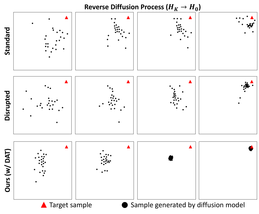
Visualization of the Mesh Distribution Diffusion Process. We visualize three variations of the diffusion process: (1) Standard baseline where we perform standard diffusion without any alignment with prior distribution . (2) Disrupted baseline where we directly modify the samples to be closer to prior distribution at every step via an loss. (3) Ours (w/ DAT), which is our method. To visualize the mesh distributions, we map the mesh samples to 2D space via the t-SNE algorithm [56], where each dot represents a sample. As shown in the top row of Fig. 3, the generated samples of the Standard baseline are spread widely apart, showing that the mesh distribution does not converge to the target well. The Disrupted baseline receives prior distribution information during the diffusion process, and thus converges better than the Standard baseline, but the diffusion process is disrupted and thus the final mesh distribution deviates from the target (as shown in the middle row of Fig. 3). In contrast, the mesh distribution produced by our method smoothly converges towards the target (as shown in the bottom row of Fig. 3). For quantitative results, refer to Tab. 4 and Tab. 5.
Visualization of Samples. Some qualitative results of our method on Human3.6M and 3DPW are shown in Fig. 2. We observe that our method can handle challenging cases, e.g., under heavy occlusions or with noisy background, showing its strong ability to handle uncertainty.
Inference Speed. Here, we conduct experiments on a single GeForce RTX 3090 card and compare the speed of our proposed method (HMDiff with DAT) with existing methods in terms of the accuracy metric (MPJPE) and inference speed (FPS) in Tab. 6. Our method can achieve a competitive speed compared with the current SOTA [6] while significantly outperforming it (as shown in Tab. 1 and Tab. 2).
| Method | Human3.6M(MPJPE) | FPS |
|---|---|---|
| [6] | 52.2 | 23 |
| Ours | 49.3 | 18 |
6 Conclusion
We present HMDiff, a novel diffusion-based framework that frames mesh recovery as a reverse diffusion process to tackle monocular HMR. We infuse prior distribution information via our proposed DAT during the diffusion process to obtain improved performance. Extensive experiments show that the proposed method achieves state-of-the-art performance on three widely used benchmark datasets.
7 Acknowledgements
This work was supported by the Singapore Ministry of Education (MOE) AcRF Tier 2 under Grant MOE-T2EP20222-0009, the National Research Foundation Singapore through AI Singapore Programme under Grant AISG-100E-2020-065, and SUTD SKI Project under Grant SKI 2021_02_06.
References
- [1] Jake K Aggarwal and Quin Cai. Human motion analysis: A review. Computer vision and image understanding, 73(3):428–440, 1999.
- [2] Mykhaylo Andriluka, Leonid Pishchulin, Peter Gehler, and Bernt Schiele. 2d human pose estimation: New benchmark and state of the art analysis. In Proceedings of the IEEE Conference on computer Vision and Pattern Recognition, pages 3686–3693, 2014.
- [3] Dragomir Anguelov, Praveen Srinivasan, Daphne Koller, Sebastian Thrun, Jim Rodgers, and James Davis. Scape: shape completion and animation of people. In ACM SIGGRAPH 2005 Papers, pages 408–416. 2005.
- [4] Benjamin Biggs, David Novotny, Sebastien Ehrhardt, Hanbyul Joo, Ben Graham, and Andrea Vedaldi. 3d multi-bodies: Fitting sets of plausible 3d human models to ambiguous image data. Advances in Neural Information Processing Systems, 33:20496–20507, 2020.
- [5] Adnane Boukhayma, Rodrigo de Bem, and Philip HS Torr. 3d hand shape and pose from images in the wild. In Proceedings of the IEEE/CVF Conference on Computer Vision and Pattern Recognition, pages 10843–10852, 2019.
- [6] Junhyeong Cho, Kim Youwang, and Tae-Hyun Oh. Cross-attention of disentangled modalities for 3d human mesh recovery with transformers. In Computer Vision–ECCV 2022: 17th European Conference, Tel Aviv, Israel, October 23–27, 2022, Proceedings, Part I, pages 342–359. Springer, 2022.
- [7] Hongsuk Choi, Gyeongsik Moon, and Kyoung Mu Lee. Pose2mesh: Graph convolutional network for 3d human pose and mesh recovery from a 2d human pose. In European Conference on Computer Vision, pages 769–787. Springer, 2020.
- [8] Hongsuk Choi, Gyeongsik Moon, JoonKyu Park, and Kyoung Mu Lee. Learning to estimate robust 3d human mesh from in-the-wild crowded scenes. In Proceedings of the IEEE/CVF Conference on Computer Vision and Pattern Recognition, pages 1475–1484, 2022.
- [9] Hyungjin Chung, Jeongsol Kim, Michael Thompson Mccann, Marc Louis Klasky, and Jong Chul Ye. Diffusion posterior sampling for general noisy inverse problems. In International Conference on Learning Representations, 2023.
- [10] Lin Geng Foo, Hossein Rahmani, and Jun Liu. Ai-generated content (aigc) for various data modalities: A survey. arXiv preprint arXiv:2308.14177, 2023.
- [11] Jia Gong, Lin Geng Foo, Zhipeng Fan, Qiuhong Ke, Hossein Rahmani, and Jun Liu. Diffpose: Toward more reliable 3d pose estimation. In Proceedings of the IEEE/CVF Conference on Computer Vision and Pattern Recognition (CVPR), June 2023.
- [12] John C Gower. Generalized procrustes analysis. Psychometrika, 40:33–51, 1975.
- [13] Tianpei Gu, Guangyi Chen, Junlong Li, Chunze Lin, Yongming Rao, Jie Zhou, and Jiwen Lu. Stochastic trajectory prediction via motion indeterminacy diffusion. In Proceedings of the IEEE/CVF Conference on Computer Vision and Pattern Recognition, pages 17113–17122, 2022.
- [14] Peng Guan, Alexander Weiss, Alexandru O Balan, and Michael J Black. Estimating human shape and pose from a single image. In 2009 IEEE 12th International Conference on Computer Vision, pages 1381–1388. IEEE, 2009.
- [15] Chuchu Han, Xin Yu, Changxin Gao, Nong Sang, and Yi Yang. Single image based 3d human pose estimation via uncertainty learning. Pattern Recognition, 132:108934, 2022.
- [16] Yana Hasson, Gul Varol, Dimitrios Tzionas, Igor Kalevatykh, Michael J Black, Ivan Laptev, and Cordelia Schmid. Learning joint reconstruction of hands and manipulated objects. In Proceedings of the IEEE/CVF conference on computer vision and pattern recognition, pages 11807–11816, 2019.
- [17] Jonathan Ho, Ajay Jain, and Pieter Abbeel. Denoising diffusion probabilistic models. Advances in Neural Information Processing Systems, 33:6840–6851, 2020.
- [18] Yinghao Huang, Federica Bogo, Christoph Lassner, Angjoo Kanazawa, Peter V Gehler, Javier Romero, Ijaz Akhter, and Michael J Black. Towards accurate marker-less human shape and pose estimation over time. In 2017 international conference on 3D vision (3DV), pages 421–430. IEEE, 2017.
- [19] Yinghao Huang, Manuel Kaufmann, Emre Aksan, Michael J Black, Otmar Hilliges, and Gerard Pons-Moll. Deep inertial poser: Learning to reconstruct human pose from sparse inertial measurements in real time. ACM Transactions on Graphics (TOG), 37(6):1–15, 2018.
- [20] Catalin Ionescu, Dragos Papava, Vlad Olaru, and Cristian Sminchisescu. Human3.6m: Large scale datasets and predictive methods for 3d human sensing in natural environments. IEEE transactions on pattern analysis and machine intelligence, 36(7):1325–1339, 2013.
- [21] Angjoo Kanazawa, Michael J Black, David W Jacobs, and Jitendra Malik. End-to-end recovery of human shape and pose. In Proceedings of the IEEE conference on computer vision and pattern recognition, pages 7122–7131, 2018.
- [22] Bahjat Kawar, Michael Elad, Stefano Ermon, and Jiaming Song. Denoising diffusion restoration models. Advances in Neural Information Processing Systems, 35:23593–23606, 2022.
- [23] Rawal Khirodkar, Shashank Tripathi, and Kris Kitani. Occluded human mesh recovery. In Proceedings of the IEEE/CVF conference on computer vision and pattern recognition, pages 1715–1725, 2022.
- [24] Arno Knapitsch, Jaesik Park, Qian-Yi Zhou, and Vladlen Koltun. Tanks and temples: Benchmarking large-scale scene reconstruction. ACM Transactions on Graphics (ToG), 36(4):1–13, 2017.
- [25] Muhammed Kocabas, Nikos Athanasiou, and Michael J Black. Vibe: Video inference for human body pose and shape estimation. In Proceedings of the IEEE/CVF conference on computer vision and pattern recognition, pages 5253–5263, 2020.
- [26] Muhammed Kocabas, Chun-Hao P Huang, Otmar Hilliges, and Michael J Black. Pare: Part attention regressor for 3d human body estimation. In Proceedings of the IEEE/CVF International Conference on Computer Vision, pages 11127–11137, 2021.
- [27] Nikos Kolotouros, Georgios Pavlakos, Michael J Black, and Kostas Daniilidis. Learning to reconstruct 3d human pose and shape via model-fitting in the loop. In Proceedings of the IEEE/CVF international conference on computer vision, pages 2252–2261, 2019.
- [28] Nikos Kolotouros, Georgios Pavlakos, and Kostas Daniilidis. Convolutional mesh regression for single-image human shape reconstruction. In Proceedings of the IEEE/CVF Conference on Computer Vision and Pattern Recognition, pages 4501–4510, 2019.
- [29] Jogendra Nath Kundu, Siddharth Seth, Pradyumna YM, Varun Jampani, Anirban Chakraborty, and R. Venkatesh Babu. Uncertainty-aware adaptation for self-supervised 3d human pose estimation. In Proceedings of the IEEE/CVF Conference on Computer Vision and Pattern Recognition (CVPR), pages 20448–20459, June 2022.
- [30] Christoph Lassner, Javier Romero, Martin Kiefel, Federica Bogo, Michael J Black, and Peter V Gehler. Unite the people: Closing the loop between 3d and 2d human representations. In Proceedings of the IEEE conference on computer vision and pattern recognition, pages 6050–6059, 2017.
- [31] Gun-Hee Lee and Seong-Whan Lee. Uncertainty-aware human mesh recovery from video by learning part-based 3d dynamics. In Proceedings of the IEEE/CVF International Conference on Computer Vision, pages 12375–12384, 2021.
- [32] Xiang Lisa Li, John Thickstun, Ishaan Gulrajani, Percy Liang, and Tatsunori B Hashimoto. Diffusion-lm improves controllable text generation. arXiv preprint arXiv:2205.14217, 2022.
- [33] Kevin Lin, Lijuan Wang, and Zicheng Liu. End-to-end human pose and mesh reconstruction with transformers. In Proceedings of the IEEE/CVF Conference on Computer Vision and Pattern Recognition, pages 1954–1963, 2021.
- [34] Kevin Lin, Lijuan Wang, and Zicheng Liu. Mesh graphormer. In Proceedings of the IEEE/CVF International Conference on Computer Vision, pages 12939–12948, 2021.
- [35] Tsung-Yi Lin, Michael Maire, Serge Belongie, James Hays, Pietro Perona, Deva Ramanan, Piotr Dollár, and C Lawrence Zitnick. Microsoft coco: Common objects in context. In Computer Vision–ECCV 2014: 13th European Conference, Zurich, Switzerland, September 6-12, 2014, Proceedings, Part V 13, pages 740–755. Springer, 2014.
- [36] Matthew Loper, Naureen Mahmood, Javier Romero, Gerard Pons-Moll, and Michael J Black. Smpl: A skinned multi-person linear model. ACM transactions on graphics (TOG), 34(6):1–16, 2015.
- [37] Andreas Lugmayr, Martin Danelljan, Andres Romero, Fisher Yu, Radu Timofte, and Luc Van Gool. Repaint: Inpainting using denoising diffusion probabilistic models. In Proceedings of the IEEE/CVF Conference on Computer Vision and Pattern Recognition, pages 11461–11471, 2022.
- [38] Zhengxiong Luo, Zhicheng Wang, Yan Huang, Liang Wang, Tieniu Tan, and Erjin Zhou. Rethinking the heatmap regression for bottom-up human pose estimation. In Proceedings of the IEEE/CVF conference on computer vision and pattern recognition, pages 13264–13273, 2021.
- [39] Dushyant Mehta, Oleksandr Sotnychenko, Franziska Mueller, Weipeng Xu, Srinath Sridhar, Gerard Pons-Moll, and Christian Theobalt. Single-shot multi-person 3d pose estimation from monocular rgb. In 2018 International Conference on 3D Vision (3DV), pages 120–130. IEEE, 2018.
- [40] Gyeongsik Moon and Kyoung Mu Lee. I2l-meshnet: Image-to-lixel prediction network for accurate 3d human pose and mesh estimation from a single rgb image. In European Conference on Computer Vision, pages 752–768. Springer, 2020.
- [41] Richard A Newcombe, Shahram Izadi, Otmar Hilliges, David Molyneaux, David Kim, Andrew J Davison, Pushmeet Kohi, Jamie Shotton, Steve Hodges, and Andrew Fitzgibbon. Kinectfusion: Real-time dense surface mapping and tracking. In 2011 10th IEEE international symposium on mixed and augmented reality, pages 127–136. Ieee, 2011.
- [42] Mohamed Omran, Christoph Lassner, Gerard Pons-Moll, Peter Gehler, and Bernt Schiele. Neural body fitting: Unifying deep learning and model based human pose and shape estimation. In 2018 international conference on 3D vision (3DV), pages 484–494. IEEE, 2018.
- [43] Georgios Pavlakos, Luyang Zhu, Xiaowei Zhou, and Kostas Daniilidis. Learning to estimate 3d human pose and shape from a single color image. In Proceedings of the IEEE conference on computer vision and pattern recognition, pages 459–468, 2018.
- [44] Duo Peng, Ping Hu, Qiuhong Ke, and Jun Liu. Diffusion-based image translation with label guidance for domain adaptive semantic segmentation. In Proceedings of the IEEE/CVF International Conference on Computer Vision (ICCV), 2023.
- [45] Anurag Ranjan, Timo Bolkart, Soubhik Sanyal, and Michael J Black. Generating 3d faces using convolutional mesh autoencoders. In Proceedings of the European conference on computer vision (ECCV), pages 704–720, 2018.
- [46] Javier Romero, Dimitrios Tzionas, and Michael J. Black. Embodied hands: Modeling and capturing hands and bodies together. ACM Transactions on Graphics, (Proc. SIGGRAPH Asia), 36(6), Nov. 2017.
- [47] Daeyun Shin, Zhile Ren, Erik B Sudderth, and Charless C Fowlkes. 3d scene reconstruction with multi-layer depth and epipolar transformers. In Proceedings of the IEEE/CVF International Conference on Computer Vision, pages 2172–2182, 2019.
- [48] Leonid Sigal, Alexandru Balan, and Michael Black. Combined discriminative and generative articulated pose and non-rigid shape estimation. Advances in neural information processing systems, 20, 2007.
- [49] Uriel Singer, Adam Polyak, Thomas Hayes, Xi Yin, Jie An, Songyang Zhang, Qiyuan Hu, Harry Yang, Oron Ashual, Oran Gafni, et al. Make-a-video: Text-to-video generation without text-video data. arXiv preprint arXiv:2209.14792, 2022.
- [50] Jascha Sohl-Dickstein, Eric Weiss, Niru Maheswaranathan, and Surya Ganguli. Deep unsupervised learning using nonequilibrium thermodynamics. In International Conference on Machine Learning, pages 2256–2265. PMLR, 2015.
- [51] Jiaming Song, Chenlin Meng, and Stefano Ermon. Denoising diffusion implicit models. In International Conference on Learning Representations, 2021.
- [52] Jiaming Song, Arash Vahdat, Morteza Mardani, and Jan Kautz. Pseudoinverse-guided diffusion models for inverse problems. In International Conference on Learning Representations, 2023.
- [53] Yang Song and Stefano Ermon. Generative modeling by estimating gradients of the data distribution. Advances in Neural Information Processing Systems, 32, 2019.
- [54] Yating Tian, Hongwen Zhang, Yebin Liu, and Limin Wang. Recovering 3d human mesh from monocular images: A survey. arXiv preprint arXiv:2203.01923, 2022.
- [55] Philip Treleaven and Jonathan Wells. 3d body scanning and healthcare applications. Computer, 40(7):28–34, 2007.
- [56] Laurens Van der Maaten and Geoffrey Hinton. Visualizing data using t-sne. Journal of machine learning research, 9(11), 2008.
- [57] Pascal Vincent. A connection between score matching and denoising autoencoders. Neural computation, 23(7):1661–1674, 2011.
- [58] Timo Von Marcard, Roberto Henschel, Michael J Black, Bodo Rosenhahn, and Gerard Pons-Moll. Recovering accurate 3d human pose in the wild using imus and a moving camera. In Proceedings of the European conference on computer vision (ECCV), pages 601–617, 2018.
- [59] Jingdong Wang, Ke Sun, Tianheng Cheng, Borui Jiang, Chaorui Deng, Yang Zhao, Dong Liu, Yadong Mu, Mingkui Tan, Xinggang Wang, et al. Deep high-resolution representation learning for visual recognition. IEEE transactions on pattern analysis and machine intelligence, 43(10):3349–3364, 2020.
- [60] Zhenbo Yu, Junjie Wang, Jingwei Xu, Bingbing Ni, Chenglong Zhao, Minsi Wang, and Wenjun Zhang. Skeleton2mesh: Kinematics prior injected unsupervised human mesh recovery. In Proceedings of the IEEE/CVF International Conference on Computer Vision, pages 8619–8629, 2021.
- [61] Andrei Zanfir, Eduard Gabriel Bazavan, Mihai Zanfir, William T Freeman, Rahul Sukthankar, and Cristian Sminchisescu. Neural descent for visual 3d human pose and shape. In Proceedings of the IEEE/CVF Conference on Computer Vision and Pattern Recognition, pages 14484–14493, 2021.
- [62] Ce Zheng, Matias Mendieta, Pu Wang, Aidong Lu, and Chen Chen. A lightweight graph transformer network for human mesh reconstruction from 2d human pose. In Proceedings of the 30th ACM International Conference on Multimedia, pages 5496–5507, 2022.
- [63] Xiaowei Zhou, Menglong Zhu, Georgios Pavlakos, Spyridon Leonardos, Konstantinos G Derpanis, and Kostas Daniilidis. Monocap: Monocular human motion capture using a cnn coupled with a geometric prior. IEEE transactions on pattern analysis and machine intelligence, 41(4):901–914, 2018.
- [64] Christian Zimmermann, Duygu Ceylan, Jimei Yang, Bryan Russell, Max Argus, and Thomas Brox. Freihand: A dataset for markerless capture of hand pose and shape from single rgb images. In Proceedings of the IEEE/CVF International Conference on Computer Vision, pages 813–822, 2019.