GARCHX-NoVaS: A Model-free Approach to Incorporate Exogenous Variables

In a seminal work, ARCH was proposed by Engle, 1982 to model volatility or $\sigma_{t}^{2}$ for a time-series in a dynamic way. Following this, many different variants were developed in the econometrics literature. The GARCH model, especially the GARCH(1,1), stands as possibly the most popular one. The classic GARCH(1,1) model as defined by Bollerslev, 1986 can be described below:

$$\begin{split}Y_{t}&=\sigma_{t}W_{t},\\ \sigma_{t}^{2}&=a+a_{1}Y_{t-1}^{2}+b_{1}\sigma_{t-1}^{2};\end{split}$$

(3)

where $a\geq 0$, $a_{1}>0$, $b_{1}>0$, and $W_{t}\sim i.i.d.~N(0,1)$. More generally, we can express the GARCH-type models as

$$Y_{t}=\sigma_{t}\eta_{t};$$

where a particular distribution of $\eta_{t}$ is not necessary and we can only assume that $\mathbb{E}(\eta_{t}^{2}|\mathscr{F}_{t-1})=1$. Usually, $\mathscr{F}_{t-1}$ is taken as the sigma-field generated by previous information $\{Y_{t-1},\ldots\}$. When additional information is available, people would like to utilize this extra knowledge to improve prediction accuracy. Subsequently, the so-called GARCHX model enters the public eye; see Francq et al., 2019 for discussions on the quasi-maximum likelihood estimation inference of GARCHX models. To simplify the analysis, we still assume the normality of $W_{t}$. After taking a vector of exogenous covariates $\bm{X}=(X_{1},\ldots,X_{m})$ into account, we can wrap the exogenous covariates into the prediction process by turning the GARCH(1,1) model into the following GARCHX(1,1,1) model:

$$\begin{split}Y_{t}&=\sigma_{t}W_{t},\\ \sigma_{t}^{2}&=a+a_{1}Y_{t-1}^{2}+b_{1}\sigma_{t-1}^{2}+\bm{c}^{T}\bm{X}_{t-1};\end{split}$$

(4)

where $\bm{X}_{t-1}$ represents $(X_{1,t-1},\ldots,X_{m,t-1})$ and $\bm{c}$ are the coefficients of these exogenous variables to be estimated. To perform a moving-window out-of-sample prediction experiment, we first need to estimate the GARCH(1,1) and GARCHX(1,1,1) models²² 2 For estimation of the GARCH and GARCHX models, we use the fGarch (Wuertz et al., 2013) and garchx packages (Sucarrat, 2020) in the R language and environment (R Core Team, 2023)., and then we compute predictions iteratively; see Section 4 for details. In this process, we assume that we know the true exogenous variables, which is feasible because we generate out-of-sample predictions. For practical applications, if needed, the future exogenous information can be estimated separately.

The model-free prediction principle was initially well developed by Politis, 2015. Later, Chen and Politis, 2019 applied this idea to multi-step ahead predictions of financial returns in the context of an ARCH-model structure. In short, the main idea behind the model-free prediction is to apply an invertible transformation function, $H_{T}$, that can map a non-$i.i.d.$ vector, $\{Y_{t}~;t=1,\ldots,T\}$, to a vector, $\{\epsilon_{t};~t=1,\ldots,T\}$, with $i.i.d.$ components (chosen as standard normal in this work). Due to the invertibility of the function, $H_{T}$, it is possible to construct a one-to-one relationship between a future value, $Y_{T+1}$, and $\epsilon_{T+1}$, i.e.,

$$Y_{T+1}=f_{T+1}(\bm{Y}_{T},\bm{X}_{T+1},\epsilon_{T+1});$$

(5)

where $\bm{Y}_{T}$ denotes all historical data $\{Y_{t};~t=1,\ldots,T\}$; $\bm{X}_{T+1}$ is the collection of all predictors, and it also contains the value of a future predictor $X_{T+1}$; the form of $f_{T+1}(\cdot)$ depends on $H^{-1}_{T}$. This relationship implies that we can also transform the prediction of $\epsilon_{T+1}$ to the prediction of $Y_{T+1}$. Assume we have $\hat{\epsilon}_{T+1}$ to the be the predictor of $\epsilon_{T+1}$, we can express the predictor of $Y_{T+1}$ as

$$\widehat{Y}_{T+1}=f_{T+1}(\bm{Y}_{T},\bm{X}_{T+1},\hat{\epsilon}_{T+1}).$$

(6)

Because the prediction of $i.i.d.$ data is standard, the $L_{1}$ (Mean Absolute Deviation) , $L_{2}$ (Mean Squared Error), or another optimal quantile predictor of $\epsilon_{T+1}$ can easily be found. We, thus, can easily obtain the corresponding optimal predictor of $Y_{T+1}$.

For multi-step ($h$-step) ahead prediction, we simply repeat this prediction process, i.e., we express $Y_{T+h}$ through a function w.r.t. $\bm{Y}_{T}$, $\bm{X}_{T+1}$ and $\{\epsilon_{T+1},\ldots,\epsilon_{T+h}\}$:

$$Y_{T+h}=f_{T+h}(\bm{Y}_{T},\bm{X}_{T+1},\epsilon_{T+1},\ldots,\epsilon_{T+h}).$$

(7)

In order to compute the prediction of $Y_{T+h}$, we take a distribution-match approach to approximate the distribution of $Y_{T+h}$. Ideally, when we know the exact distribution of the $i.i.d.$ $\epsilon$, we can use a Monte Carlo simulation to approximate the distribution of $Y_{T+h}$ based on Eq. 7. Practically speaking, when we just have the empirical transformation results, i.e., the observed sample $\{\epsilon_{t}\}_{t=1}^{T}$, bootstrap is an appropriate approach. Moreover, we can even predict $g(Y_{T+h})$, where $g(\cdot)$ is a general continuous function. For example, we can compute the $L_{1}$ and $L_{2}$ optimal predictors of $g(Y_{T+h})$ as below:

$$\begin{split}g(Y_{T+h})_{L_{2}}&=\frac{1}{M}\sum_{m=1}^{M}g(f_{T+h}(\bm{Y}_{T},\bm{X}_{T+1},\hat{\epsilon}_{T+1,m},\ldots,\hat{\epsilon}_{T+h,m})),\\ g(Y_{T+h})_{L_{1}}&=\text{Median~of~}\{g(f_{T+h}(\bm{Y}_{T},\bm{X}_{T+1},\hat{\epsilon}_{T+1,m},\ldots,\hat{\epsilon}_{T+h,m}));m=1,\ldots,M\};\end{split}$$

(8)

where $g(Y_{T+h})_{L_{2}}$ and $g(Y_{T+h})_{L_{1}}$ represent the optimal $L_{2}$ and $L_{1}$ predictor of $g(Y_{T+1})$, the $\{\hat{\epsilon}_{T+1,m}\}_{m=1}^{M}$ are generated by bootstrap or Monte Carlo simulation, and $M$ is some large number (2000 in our empirical analysis). For further discussion, see Politis, 2015.

To the best of our knowledge, the model-free prediction idea has not been studied when the model features exogenous variables. However, it may be beneficial to take into account in the prediction process the additional information embedded in such exogenous variables. To show the NoVaS approach is still applicable, we need a transformation function that maps the targeted variables and exogenous predictors together into some simple $i.i.d.$ random variables. Under some mild conditions, we show the existence of such a transformation function based on the probability integral transform. We assume:

• •

  A1 The joint density of $\{Y_{1},\cdots,Y_{T}\}$ exists for any $T\geq 1$.

• •

  A2 For exogenous random vector $\bm{X}:=\{X_{1},\cdots,X_{m}\}$, the joint density $\{Y_{1},\cdots,Y_{T},X_{1},\cdots,X_{m}\}$ exists for any $m\geq 1$.

Then, the feasibility of NoVaS transformation with exogenous variables existing is guaranteed by 2.1 shown below:

The direct implication of 2.1 is that the Model-free prediction principle is feasible even when exogenous variables are included in the dependence dynamics. Moreover, our theorem is more general than the result from Wang and Politis, 2022 where the time series must satisfy some strict conditions. In short, we build a transformation function based on the GARCHX model structure to estimate the oracle functions $\bm{g}$ and $\bm{h}$, so we call our method GAX-NoVaS. We should mention again that the “model-free” in this context means we do not rely on an assumed underlying model to make predictions. Although a transformation function needs to be estimated, it is just a “bridge” that connects original and transformed distributions according to the distribution match idea.

For the sake of completeness, we first give a brief introduction to the NoVaS transformation (model) which is a direct application of the Model-free prediction idea explained in Section 2.2. Initially, the NoVaS transformation is developed from the ARCH model:

$$Y_{t}=W_{t}\sqrt{a+\sum_{i=1}^{p}a_{i}Y_{t-i}^{2}}.$$

(11)

here, these parameters satisfy $a\geq 0$, $a_{i}\geq 0$, for all $i=1,\ldots,p$; $W_{t}\sim i.i.d.~N(0,1)$. In other words, the structure of the ARCH model gives us a ready-made $H^{-1}_{T}$. We can express $W_{t}$ in Eq. 11 using other terms to get a potential $H_{T}$ :

$$W_{t}=\frac{Y_{t}}{\sqrt{a+\sum_{i=1}^{p}a_{i}Y_{t-i}^{2}}}~;~\text{for}~t=p+1,\ldots,T.$$

(12)

Politis, 2003 further modified Eq. 12 as follows:

$$W_{t}=\frac{Y_{t}}{\sqrt{\alpha s_{t-1}^{2}+\beta Y_{t}^{2}+\sum_{i=1}^{p}a_{i}Y_{t-i}^{2}}}~;~\text{for}~t=p+1,\ldots,T.$$

(13)

here, $\{Y_{t};~t=1,\ldots,T\}$ is the sample data; $\{W_{t};~t=p+1,\ldots,T\}$ is the transformed vector; $\alpha$ is a fixed scale invariant constant; $s_{t-1}^{2}$ is an estimator of the variance of $\{Y_{i};~i=1,\ldots,t-1\}$ and can be calculated by $(t-1)^{-1}\sum_{i=1}^{t-1}(Y_{i}-\overline{Y})^{2}$, where $\overline{Y}$ is the sample mean of $\{Y_{i};~i=1,\ldots,t-1\}$. For making Eq. 13 be a qualified function $H_{T}$, i.e., making $\{W_{t}\}_{t=p+1}^{T}$ really obey $i.i.d.$ standard normal distribution, we need to impose some restrictions on $\alpha$ and $\beta,a_{1},\ldots,a_{p}$. We first stabilize the variance by requiring:

$$\alpha\geq 0,\beta\geq 0,a_{i}\geq 0~;~\text{for all}~i\geq 1,\alpha+\beta+\sum_{i=1}^{p}a_{i}=1.$$

(14)

In application, $\{W_{t}\}_{t=p+1}^{T}$ transformed from financial log-returns by NoVaS transformation are usually uncorrelated. Therefore, if we make $\{W_{t}\}_{t=p+1}^{T}$ close to a Gaussian series i.e., normalizing $\{W_{t}\}_{t=p+1}^{T}$, we can get the desired $i.i.d.$ property. This is why this transformation is called NoVaS.

There are many criteria to measure the normality of a series. Under the observation that the distribution of financial log-returns is usually symmetric, we choose the kurtosis to be a simple distance to measure the departure of a non-skewed dataset from that of the standard normal distribution (Politis, 2015). Besides, matching marginal distribution seems sufficient to normalize the joint distribution of $\{W_{t}\}_{t=p+1}^{T}$ for practical purposes based on empirical results. If we denote the marginal distribution of $\{W_{t}\}_{t=p+1}^{T}$ and the corresponding kurtosis by $\widehat{F}_{w}$ and $\text{KURT}(W_{t})$, respectively, we then attempt to minimize $|\text{KURT}(W_{t})-3|$ to obtain the optimal combination of $\alpha,\beta,a_{1},\ldots,a_{p}$ such that $\widehat{F}_{w}$ is as close to standard normal distribution as possible. Subsequently, the NoVaS transformation can be determined.

The remaining difficulty is how to finish this optimization step to get optimal coefficients $\alpha,\beta,a_{1},\ldots,a_{p}$, especially when $p$ is large. To simplify this problem, Politis, 2015 defined an exponentially decayed form of $\{a_{i}\}_{i=1}^{p}$:

$$\alpha\neq 0,\beta=c^{\prime},a_{i}=c^{\prime}e^{-ci}~;~\text{for all}~1\leq i\leq p,c^{\prime}=\frac{1-\alpha}{\sum_{j=0}^{p}e^{-cj}}.$$

(15)

The NoVaS transformation based on coefficients defined in Eq. 15 is called Generalized Exponential NoVaS (GE-NoVaS). In other words, we can represent the $p+2$ number of coefficients by two parameters $c$ and $\alpha$, which relieve the optimization burden, but with a sacrifice that the coefficients are fixed in a decayed form. To achieve a balance between the relief of the optimization dilemma and the freedom of coefficients, inspired by the development of GARCH from ARCH, Wu and Karmakar, 2023 built a NoVaS transformation according to the GARCH model, namely GARCH-NoVaS which was shown to be more stable and accurate. Later, we specify the GAX-NoVaS transformation in detail.

Starting from Eq. 4, we take similar steps of building GA-NoVaS to find the transformation function of the GAX-NoVaS method. In order to simplify the notation, we consider the case of only one exogenous covariate $X_{t}$. The case of multiple exogenous covariates can be analyzed in an analogous way. First, we notice that we can rewrite the Eq. 4 as

$$W_{t}=\frac{Y_{t}}{\sqrt{a_{0}+a_{1}Y^{2}_{t-1}+b_{1}\sigma_{t-1}^{2}+c_{1}X_{t-1}}}.$$

(16)

We also have

$$\begin{split}&\sigma_{t-1}^{2}=a_{0}+a_{1}Y^{2}_{t-2}+b_{1}\sigma_{t-2}^{2}+c_{1}X_{t-2},\\ &\sigma_{t-2}^{2}=a_{0}+a_{1}Y^{2}_{t-3}+b_{1}\sigma_{t-3}^{2}+c_{1}X_{t-3},\\ \vdots\end{split}$$

(17)

so that we can substitute these terms into Eq. 16. We then get

$$W_{t}=\frac{Y_{t}}{\sqrt{\frac{a_{0}}{1-b_{1}}+\sum_{i=1}^{p}a_{1}b_{1}^{i-1}Y^{2}_{t-i}+\sum_{i=1}^{p}c_{1}b_{1}^{i-1}X_{t-i}}},$$

(18)

where $p$ is a large constant that is used to truncate the infinite summation (we take $p=q$ in this work), because $a_{1}$ and $b_{1}$ need to be less than one to guarantee the stationary property of the GARCHX series. In line with the NoVaS transformation, we finally write the transformation function as follows:

$$W_{t}=\frac{Y_{t}}{\sqrt{\alpha s_{t-1,Y}+\beta s_{t-1,X}+\sum_{i=1}^{p}a_{1}b_{1}^{i-1}Y^{2}_{t-i}+\sum_{i=1}^{p}c_{1}b_{1}^{i-1}Y_{t-i}}},$$

(19)

where $s^{2}_{t-1,Y}$ and $s^{2}_{t-1,X}$ are the sample variance of $\{Y_{1},\ldots,Y_{t-1}\}$ and $\{X_{1},\ldots,X_{t-1}\}$, respectively. Thus, we can use Eq. 19 as the transformation function for the GARCHX model, where $\{W_{t}\}$ is the transformed series. We want to make $\{W_{t}\}$ $i.i.d.$ normal, so that the one-step (conditional) prediction $\widehat{Y}_{T+1}$ can be expressed as

$$\widehat{Y}_{T+1}=\widehat{W}_{T+1}\sqrt{\alpha s^{2}_{T-1,Y}+\beta s^{2}_{T-1,X}+\sum_{i=1}^{p}a_{1}b_{1}^{i-1}Y^{2}_{T-i}+\sum_{i=1}^{p}c_{1}b_{1}^{i-1}X_{T-i}},$$

(20)

where $\widehat{W}_{T+1}$ is the optimal point prediction based on $i.i.d.$ $\{W_{1},\ldots,W_{T}\}$. Multi-step-ahead predictions can be computed as explained in Section 2.2.

The final question left now is how to find a transformation function that indeed makes $\{W_{t}\}$ $i.i.d.$ normal. While we have made some brief remarks on this question in Section 3.1, we next provide a full explanation with a focus on the GAX-NoVaS method. Our goal is to determine the coefficients, $\alpha,\beta,a_{1},b_{1},c_{1}$, of Eq. 19 to obtain the desired transformation. The most important step is to minimize $|\text{KURT}(W_{t})-3|$, where $3$ is the kurtosis of normal distribution. For this optimization, we use the numerical technique to find the optimal coefficients.³³ 3 We use the nloptr package (Ypma et al., 2014) for R. In operation, one may obtain some extremely large values from the transformed series $\{W_{t}\}$, and such outliers may spoil the normality of the transformed series and may also influence prediction performance. Thus, before moving on to the prediction step, we truncate the transformed series by the 0.99 and 0.01 quantile values of a normal distribution with mean and standard deviation given by the sample mean and sample standard deviation of $\{W_{t}\}$.

If we have sample $\{Y_{1},\ldots,Y_{N}\}$ at hand, in order to fully exhaust the dataset, we can focus on moving-window out-of-sample predictions, i.e., we use $\{Y_{1},\cdots,Y_{T}\}$ to predict {$Y_{T+1}^{2},\cdots,Y_{T+h}^{2}\}$, then we use $\{Y_{2},\cdots,Y_{T+1}\}$ to predict $\{Y_{T+2}^{2},\cdots,Y_{T+h+1}^{2}\}$, and so on until we reach the end of the sample (that is, until we use $\{Y_{N-T+h+1},\cdots,Y_{N-h}\}$ to predict $\{Y^{2}_{N-h+1},\ldots,Y^{2}_{N}\}$). Here, $T$ denotes the moving window size; we fix its size as 250; $h$ is the prediction horizon, i.e., 1, 5, 20 in our setting. Sometimes, we may not have enough data available to perform predictions. Thus, the window size $T=250$ is designed to see if this method is stable and can still return accurate predictions even with short data. A 250-size moving window is in line with around one year of daily financial data. In this perspective, it is important to keep in mind that a 250-size moving window is practically meaningful since the time series may not be stationary on a wider span.

In addition, we are not only interested in the one-step-ahead prediction $h=1$ but also multi-step-ahead prediction $h>1$. From a practical aspect of forecasting volatility, as mentioned above in our introduction Section 1, the long-term prediction ($h$ takes a large value) is important and can guide future strategic decisions. Before this evaluation, we start by writing time-aggregated predictions as follows:

$$\overline{\widehat{Y}}_{T,h}^{2}=\sum_{k=1}^{h}\widehat{Y}_{T+k}^{2}/h,$$

(21)

where $\overline{\widehat{Y}}_{T,h}^{2}$ is the $h$-step ahead time-aggregated volatility prediction starting from $Y_{T}$. For example, if the total number of data $N=1000$ and we consider the 6-step-ahead moving window time-aggregated predictions with $T=500,$ we need to find predictions $\overline{\widehat{Y}}_{T,6}^{2}$ for $T=500,\ldots,994$.

We hope the time-aggregated volatility prediction is close to the true aggregated value calculated from the realized average squared log-returns $\overline{Y}_{l,h}^{2}=\sum_{k=1}^{h}(Y_{T+k}^{2}/h)$. To evaluate the accuracy, we can consider the specific mean of squared prediction errors (MSPE) shown below, with this statistic aiming to compare the prediction performance in an absolute way:

$$P=\frac{1}{N-h-T+1}\sum_{l=T}^{N-h}(\overline{\widehat{Y}}_{l,h}^{2}-\overline{Y}_{l,h}^{2})^{2},$$

(22)

where $\overline{\widehat{Y}}_{l,h}^{2}$ and $\overline{Y}_{l,h}^{2}$ denote the predicted and true time-aggregated values for each moving-window forecasting, respectively.

In this part, we present three data-generating models to simulate data and then evaluate the performance of various methods considered in this paper. Due to the true data-generating process being known to us, we can simulate any size of the sample and compare predictions from various methods with oracle values. Besides, we remove the variance term $\beta s^{2}_{T-1,X}$ of Eq. 19 when we do the transformations since the prediction performance hardly changes with or without $\beta s^{2}_{T-1,X}$. Three true underlying models are presented below:

• Model 1: Standard GARCH(1,1) with Student-$t$ errors
  $Y_{t}=\sigma_{t}\epsilon_{t},$ $~\sigma_{t}^{2}=0.00001+0.73\sigma_{t-1}^{2}+0.1Y_{t-1}^{2}+c|X_{t-1}|,$
  $X_{t-1}\sim i.i.d.~N(0,1)$;$~\{\epsilon_{t}\}\sim i.i.d.~t$ distribution with four degrees of freedom
  $c=1$.

• Model 2: Standard GARCH(1,1) with Student-$t$ errors
  $Y_{t}=\sigma_{t}\epsilon_{t},$ $~\sigma_{t}^{2}=0.00001+0.8895\sigma_{t-1}^{2}+0.1Y_{t-1}^{2}+c|X_{t-1}|,$
  $X_{t-1}\sim i.i.d.~N(0,1)$;$~\{\epsilon_{t}\}\sim i.i.d.~t$ distribution with four degrees of freedom
  $c=1$.

• Model 3: Time-varying GARCHX(1,1) with standard normal exogenous variables:
  $Y_{t}=\sigma_{t}\epsilon_{t},~\sigma_{t}^{2}=b_{t}\sigma_{t-1}^{2}+a_{t}Y_{t-1}^{2}+c|X_{t-1}|,$
  $X_{t-1}\sim i.i.d.~N(0,1)$; $\{\epsilon_{t}\}\sim i.i.d.$ $t$ distribution with five degrees freedom;
  $c=1;g_{t}=t/n$; $a_{t}=0.1-0.05g_{t}$; $b_{t}=0.7+0.2g_{t},~n$ is the total length of the time series.

To check the robustness of methods on model misspecification, we intend to take the innovation distribution of simulation models as the $t$-distribution. Besides this purpose, we argue that the $t$ distribution as the innovation to mimic the real-world cases is more appropriate since real data usually show the heavy tail phenomenon. Models 1 and 2 are from a standard GARCH where in Model 2 we intended to explore a scenario that $\alpha_{1}+\beta_{1}$ is very close to 1 and thus mimics what would happen for the iGARCH situation. In addition, we make the coefficients of the GARCHX model change linearly in Mode-3 so that we can observe the ability of different methods to handle the data generated from a time-varying model which is more coherent to the real-world situation. To sync with the empirical studies later, we simulate a time series with a length $T=4694$. We take the moving-window size $T=250$. MSPE of GARCH, GARCHX and GAX-NoVaS methods with three simulation settings are presented below:

From Table 1, it is clear that the GAX-NoVaS is much better than GARCH and even the classical GARCHX models according to the MSPE criterion. Interestingly, the GARCHX model is even much worse than the GARCH model for some specific cases, e.g., the 20-step-ahead prediction of Model-3. By taking a deeper analysis, we find the terrible performance GARCHX method is due to some extremely large predictions. On the other hand, the prediction returned by GAX-NoVaS is more stable. The superiority is further shown in Section 5 with three real datasets and various exogenous predictors.

Since the focus of this paper is exploring a new approach to incorporate exogenous variables, we take the DM test to evaluate the performance of GARCHX and GAX-NoVaS methods more formally; see Diebold and Mariano, 2002 for the technical details of the DM-test⁴⁴ 4 We perform the DM-test with the function DM-test in the R package multDM.. The DM-test results on comparing GARCHX and GAX-NoVaS for forecasting three simulated datasets are tabularized in Table 5. These tests further verify the advantage of our methods on forecasting with exogenous variables, especially for a long-prediction horizon.

The ongoing Ukraine-Russia has led many countries in Europe, particularly Germany, to adjust their military and security, as well as energy policies in light of new geopolitical risks, with such adjustments entailing large costs to the macroeconomy and financial markets, as depicted by Grebe et al., 2024. In this regard, these authors, first, assemble a data set of more than eight million German Twitter posts related to the war in Ukraine to construct a daily index of uncertainty about the war as perceived by German Twitter based on using state-of-the-art methods of textual analysis. Grebe et al., 2024 show that an increase in uncertainty has strong effects on financial markets, associated with a significant decline in economic activity as well as an increase in expected inflation. We utilize this index (Ukraine)⁵⁵ 5 The data is available for download from: https://www.uni-giessen.de/de/fbz/fb02/fb/professuren/vwl/tillmann/forschung/ukraine-uncertainty-index. in our empirical analysis to forecast stock market volatility of not only Germany, but two of its neighbors namely, Austria and Switzerland, over the daily period of 1st January, 2021 to 28th February, 2023. The national stock market indexes (ATX (Austria), DAX (Germany), SMI (Switzerland)) of these three countries, for which we compute log-returns to feed into our volatility models were derived from the Bloomberg terminal. With the focus being on geopolitical risks, we also utilized the daily newspapers-based geopolitical risks index (GPRD) of Caldara and Iacoviello, 2022⁶⁶ 6 The data can be accessed from: https://www.matteoiacoviello.com/gpr.htm., which, in turn, allowed us to analyze a longer data sample covering 2nd January, 2006 to 10th August, 2023. The starting date of this longer sample, and the choice of these three countries, were also motivated by the availability of Google searches-based daily data on economic activity (Trend) for all three countries, and inflation (Inflation) for Germany and Switzerland,⁷⁷ 7 The data can be downloaded from: https://www.trendecon.org/. which are used as additional predictors to ensure that our results are not only limited to geopolitical risks.

We present three log-return series of Germany, Switzerland and Austria from 2nd January, 2006 to 10th August, 2023 in Figs. 1, 2 and 3. The volatility clustering phenomena observed in all plots reveals the heteroskedasticity within these three series. To investigate the property of three long return series, we provide the summary statistics, e.g., the mean, skewness, and kurtosis in Table 3. To verify the heteroskedasticity with all series more directly, we split the whole time period into four equal-length sub-periods and denote the sample variance of all four sub-periods by $V_{i}$, $i=1,\ldots,4$. These statistics are also provided in Table 3. Towards statistical tests, we also perform modified Ljung-Box (m-LB) and ARCH Lagrange Multiplier (ALM) tests to check the autocorrelation and ARCH effects of squared return series. For the m-LB test, we consider the lag order 20. For the ALM test, we consider the maximum lag order 10. These two tests are performed in R with functions lbtest and Lm.test, respectively. The p-values of tests are presented. Summarizing Table 3, the large kurtosis values indicate the heavy-tailed property for all three log-return series. The variance of return series in different time regions changes notably, indicating the heteroskedasticity. The ALM test with a pretty small p-value also confirms the heteroskedasticity for all return series. The m-LB test shows strong evidence of autocorrelation within all squared return series.

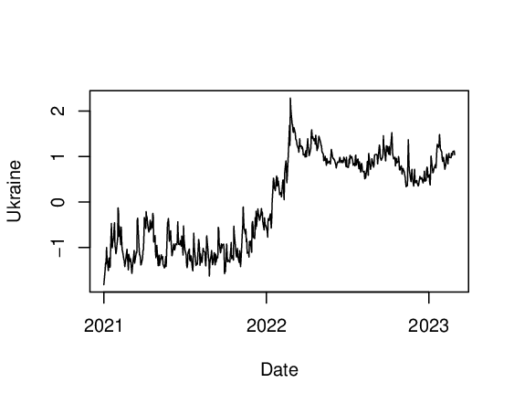
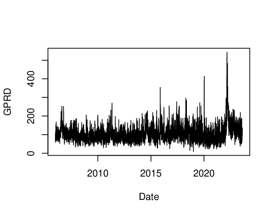
To show the fluctuations behind the Ukraine index and GPRD index, we present two plots in Figs. 4 and 5 below. As one can see from there, these two indices fluctuate severely around the beginning of 2022 which corresponds with the real-world event. Later, we attempt to use this information to forecast the stock market volatility of three countries.

We first consider the forecasting exercise with the short period (1st January, 2021 to 28th February, 2023) data described in Section 5.1. Then, the analysis of three long returns series is given in Section 5.2.2.

References

- Angus, (1994) Angus, J. E. (1994). The probability integral transform and related results. SIAM review, 36(4):652–654.
- Bollerslev, (1986) Bollerslev, T. (1986). Generalized autoregressive conditional heteroskedasticity. Journal of Econometrics, 31(3):307–327.
- Bouri et al., (2020) Bouri, E., Cepni, O., Gupta, R., and Jalkh, N. (2020). Geopolitical risks and stock market volatility in the g7 countries: A century of evidence from a time-varying nonparametric panel data model. Edited by Atin Basuchoudhary and Gunther G. Schulze.
- Box et al., (2015) Box, G. E., Jenkins, G. M., Reinsel, G. C., and Ljung, G. M. (2015). Time Series Analysis: Forecasting and Control. John Wiley & Sons.
- Caldara and Iacoviello, (2022) Caldara, D. and Iacoviello, M. (2022). Measuring geopolitical risk. American Economic Review, 112(4):1194–1225.
- Chen and Politis, (2019) Chen, J. and Politis, D. N. (2019). Optimal Multi-step-ahead Prediction of ARCH/GARCH Models and NoVaS Transformation. Econometrics, 7(3):1–23.
- Christos et al., (2019) Christos, B., Christina, C., Rangan, G., and Tahir, S. (2019). Geopolitical risks, returns, and volatility in emerging stock markets: Evidence from a panel garch model. Emerging Markets Finance and Trade, 55(8):1841–1856.
- Chudý et al., (2020) Chudý, M., Karmakar, S., and Wu, W. B. (2020). Long-term prediction intervals of economic time series. Empirical Economics, 58(1):191–222.
- Diebold and Mariano, (2002) Diebold, F. X. and Mariano, R. S. (2002). Comparing predictive accuracy. Journal of Business & economic statistics, 20(1):134–144.
- Engle and Patton, (2001) Engle, R. and Patton, A. (2001). What good is a volatility model? Quantitative Finance, 1:47–63.
- Engle, (1982) Engle, R. F. (1982). Autoregressive conditional heteroscedasticity with estimates of the variance of united kingdom inflation. Econometrica: Journal of the econometric society, pages 987–1007.
- Engle et al., (2013) Engle, R. F., Ghysels, E., and Sohn, B. (2013). Stock market volatility and macroeconomic fundamentals. Review of Economics and Statistics, 95(3):776–797.
- Engle and Patton, (2007) Engle, R. F. and Patton, A. J. (2007). What good is a volatility model? In Forecasting volatility in the financial markets, pages 47–63. Elsevier.
- Francq et al., (2019) Francq, C. et al. (2019). Qml inference for volatility models with covariates. Econometric Theory, 35(1):37–72.
- Fryzlewicz et al., (2008) Fryzlewicz, P., Sapatinas, T., Rao, S. S., et al. (2008). Normalized least-squares estimation in time-varying ARCH models. The Annals of Statistics, 36(2):742–786.
- González-Rivera et al., (2004) González-Rivera, G., Lee, T.-H., and Mishra, S. (2004). Forecasting volatility: A reality check based on option pricing, utility function, value-at-risk, and predictive likelihood. International Journal of Forecasting, 20(4):629–645.
- Grebe et al., (2024) Grebe, M., Kandemir, S., and Tillmann, P. (2024). Uncertainty about the war in ukraine: Measurement and effects on the german economy. Journal of Economic Behavior & Organization, 217(C):493–506.
- Gulay and Emec, (2018) Gulay, E. and Emec, H. (2018). Comparison of forecasting performances: Does normalization and variance stabilization method beat garch (1, 1)-type models? empirical evidence from the stock markets. Journal of Forecasting, 37(2):133–150.
- Herrera et al., (2018) Herrera, A. M., Hu, L., and Pastor, D. (2018). Forecasting crude oil price volatility. International Journal of Forecasting, 34(4):622–635.
- Karmakar et al., (2022) Karmakar, S., Chudý, M., and Wu, W. B. (2022). Long-term prediction intervals with many covariates. Journal of Time Series Analysis, 43(4):587–609.
- Karmakar and Roy, (2021) Karmakar, S. and Roy, A. (2021). Bayesian Modelling of Time-Varying Conditional Heteroscedasticity. Bayesian Analysis, 1(1):1–29.
- Lim and Sek, (2013) Lim, C. M. and Sek, S. K. (2013). Comparing the Performances of GARCH-type Models in Capturing the Stock Market Volatility in Malaysia. Procedia Economics and Finance, 5:478–487.
- Mehmet et al., (2018) Mehmet, B., Rangan, G., Christian, P., and E, W. M. (2018). Terror attacks and stock-market fluctuations: Evidence based on a nonparametric causality-in-quantiles test for the g7 countries. The European Journal of Finance, 24(4):333–346.
- Peters, (2001) Peters, J.-P. (2001). Estimating and forecasting volatility of stock indices using asymmetric GARCH models and (Skewed) Student-t densities. Preprint, University of Liege, Belgium, 3:19–34.
- Politis, (2003) Politis, D. N. (2003). A normalizing and variance-stabilizing transformation for financial time series. In Recent Advances and Trends in Nonparametric Statistics, pages 335–347. Elsevier Inc.
- Politis, (2015) Politis, D. N. (2015). The model-free prediction principle. In Model-Free Prediction and Regression, pages 13–30. Springer.
- R Core Team, (2023) R Core Team (2023). R: A Language and Environment for Statistical Computing. R Foundation for Statistical Computing, Vienna, Austria.
- Salisu et al., (2022) Salisu, A. A., Ogbonna, A. E., Lasisi, L., and Olaniran, A. (2022). Geopolitical risk and stock market volatility in emerging markets: A garch–midas approach. The North American Journal of Economics and Finance, 62:101755.
- Sucarrat, (2020) Sucarrat, G. (2020). garchx: Flexible and robust garch-x modelling.
- Wang and Politis, (2022) Wang, Y. and Politis, D. N. (2022). Model-free bootstrap for a general class of stationary time series. Bernoulli, 28(2):744–770.
- Wu and Karmakar, (2021) Wu, K. and Karmakar, S. (2021). Model-free time-aggregated predictions for econometric datasets. Forecasting, 3(4):920–933.
- Wu and Karmakar, (2023) Wu, K. and Karmakar, S. (2023). A model-free approach to do long-term volatility forecasting and its variants. Financial Innovation, 9(1):1–38.
- Wu and Politis, (2023) Wu, K. and Politis, D. N. (2023). Bootstrap prediction inference of non-linear autoregressive models. arXiv preprint arXiv:2306.04126.
- Wuertz et al., (2013) Wuertz, D., RUnit, S., and Chalabi, M. Y. (2013). Package ‘fgarch’. Technical report, Technical report, working paper/manual, 09.11. 2009. URL http://cran. r ….
- Ypma et al., (2014) Ypma, J., Borchers, H. W., and Eddelbuettel, D. (2014). nloptr: R interface to nlopt. R package version, 1(4).
- Yule, (1927) Yule, G. U. (1927). Vii. on a method of investigating periodicities disturbed series, with special reference to wolfer’s sunspot numbers. Philosophical Transactions of the Royal Society of London. Series A, Containing Papers of a Mathematical or Physical Character, 226(636-646):267–298.
- Zhang et al., (2023) Zhang, Y., He, J., He, M., and Li, S. (2023). Geopolitical risk and stock market volatility: A global perspective. Finance Research Letters, 53:103620.