Genome replication in asynchronously growing microbial populations
Abstract
Biological cells replicate their genomes in a well-planned manner. The DNA replication program of an organism determines the timing at which different genomic regions are replicated, with fundamental consequences for cell homeostasis and genome stability. Qualitatively, in a growing cell culture, one expects that genomic regions that are replicated early should be more abundant than regions that are replicated late. This abundance pattern can be experimentally measured using deep sequencing. However, a general quantitative theory to explain these data is still lacking. In this paper, we predict the abundance of DNA fragments in asynchronously growing cultures from any given stochastic model of the DNA replication program. As key examples, we present stochastic models of the DNA replication programs in Escherichia coli and in budding yeast. In both cases, our approach leads to analytical predictions that are in excellent agreement with experimental data and permit to infer key information about the replication program. In particular, our method is able to infer the locations of known replication origins in budding yeast with high accuracy. These examples demonstrate that our method can provide insight into a broad range of organisms, from bacteria to eukaryotes.
I Introduction
The genome of an organism contains precious information about its functioning. Genomes need to be reliably and quickly replicated for cells to pass biological information to the next generation. Replication of a genome proceeds according to a certain plan, termed the “replication program” Bechhoefer and Rhind 2012; Baker et al. 2012; Gispan et al. 2017; Hulke et al. 2020. For example, most bacteria have a circular genome, where two replisomes initiate replication by binding at the same origin site Xu and Dixon 2018. They replicate the genome in opposite directions. Replication is completed when they meet, after each of them has copied approximately half of the genome. The replication program is carefully orchestrated, but not completely deterministic. Stochasticity is particularly relevant in eukaryotes and archaea, where many origin sites are present in each chromosome Gilbert 2001; Costa and Diffley 2022. Replication can initiate at these origin sites at different times. These times are characterized by some degree of randomness Yang et al. 2010; Rhind 2022 and, depending on the circumstances, some origin sites may not be activated at all Bechhoefer and Rhind 2012.
Replication programs must be coordinated with the cell cycle in some way. For example, in bacteria, the moment in the cell cycle in which replication is initiated is carefully timed Cooper and Helmstetter 1968; Fu et al. 2023; Berger and ten Wolde 2023. In eukaryotes, replication takes place at a well-defined stage of the cell cycle (the S phase), during which different genomic regions are replicated at different times in a controlled manner Yang et al. 2010. The interplay between the replication program and the cell cycle is crucial when trying to infer the replication program from experimental observations. Many experiments study samples in which all cells are approximately at the same stage of the cell cycle. This can be achieved by either arresting the cell cycle at a certain stage or by cell sorting Hulke et al. 2020. The fraction of these synchronized cells that have copied each genome location can be then measured using deep sequencing. This approach has been extensively used to study the eukaryotic replication program Raghuraman et al. 2001; Daigaku et al. 2015; Hulke et al. 2020.
An alternative method is to measure the abundance of DNA fragments in asynchronous, exponentially growing populations. This approach, traditionally called marker frequency analysis Sueoka and Yoshikawa 1965, has been extensively applied to bacterial replication, for example to study Escherichia coli mutant lacking genes that assist DNA replication Wendel et al. 2014; Wendel et al. 2018; Midgley-Smith et al. 2018 and artificially engineered E.coli strains with multiple replication origins Dimude et al. 2018. The asynchronous approach is experimentally much simpler and avoids potential artifacts caused by the cell cycle arrest or cell sorting Hulke et al. 2020. Progress in DNA sequencing have made these experiments high-throughput and relatively inexpensive. However, the DNA sampled in these experiments originates from a mixture of cells at different stages in their life cycle, rendering the theoretical interpretation of such data problematic Rhind et al. 2010.
Theoretical approaches have attempted to describe measurements in asynchronous populations. However, these approaches either neglect stochasticity, or are limited to specific model systems. For example, we recently proposed a stochastic model describing DNA replication in growing E.coli populations Bhat et al. 2022. A broader range of bacterial systems have been studied assuming a deterministic replication program Huang et al. 2022a; Huang et al. 2022b. Finally, a model of the replication program in budding yeast adopted the working hypothesis that cells in an asynchronous population are at random, uniformly distributed stages in their cell cycle Gispan et al. 2017.
In this paper, we develop a general theory to infer the replication program from sequencing of an asynchronously growing population of cells. Our theory builds upon classic results on age-structured populations Powell 1956; Yoshikawa and Sueoka 1963; Sueoka and Yoshikawa 1965; Chandler and Pritchard 1975; Jafarpour et al. 2018, that we extend to populations of stochastically replicating genomes. Our approach requires minimal assumptions on the replication dynamics. In particular, it allows for a stochastic replication program and equally applies to bacteria and eukaryotes. We apply our method to experimental data from E. coli and budding yeast. In the case of E. coli, we propose and exactly solve a model of DNA replication that incorporates stochastic stalling. The fit of the solution to experimental data sheds light on recently observed oscillations of bacterial replisome speed. In the case of yeast, our approach permits to reliably infer the location of replication origins.
The paper is organized as follows. In Section II, we present our general theory. In Section III, we apply our framework to DNA replication in E. coli. In Section IV, we consider eukaryotic DNA replication, with budding yeast as an example. In Section V, we present possible extensions of our theory. Section VI is devoted to conclusions and future perspectives.
II DNA replication in asynchronously growing populations
II.1 General theory
(a)
(b)
 (c)
(c)
 (d)
(d)
We consider a large, growing population of cells. We call the number of cells that are present in the population at time . Each cell may contain multiple genomes, some complete and other undergoing synthesis (incomplete). We denote by the the total number of complete and incomplete genomes in the population.
Our theory is based on the following assumptions. The number of cells grows exponentially: , where is the exponential growth rate. The population grows in a steady, asynchronous manner. This assumption implies that the average number of genomes per cell must remain constant, and therefore . Genomes in the population are immortal, i.e. we neglect the rate at which they might be degraded. All genomes in the population are statistically identical, in the sense that they are all characterized by the same stochastic replication program. These assumptions are realistic in common experimental situations. Moreover, as we shall discuss in Section V, some of them can be readily relaxed, if necessary.
We now assign an age to each genome in the population. To this aim, we conventionally set the birth time of a daughter genome at the start of the replication process that generates it from a parent genome, see Fig. 1a. We note that the distinction between a “parent” and a “daughter” genome is somewhat arbitrary, as each of them is made up of a preexisting strand and a newly copied complementary one. Since genomes are immortal, the probability density of new genomes is proportional to , which is proportional to as well. It follows that the distribution of ages of genomes in the population must be proportional to . From this fact, we conclude that the distribution of genome ages in the population is
| (1) |
We now look into the DNA replication program in more details. In bacteria, replication is carried out by a pair of replisomes, that bind at a specific genome site (the origin) and proceed in opposite directions, each replicating both strands. DNA replication is substantially more complex in eukaryotes, where a large number of replisomes replicate the same chromosome, and initiation site might be activated stochastically. We summarize the effect of all these complex processes into the probability that the genome location has already been copied in a genome of age . By definition, is a non-decreasing function of . Our assumption that genomes are statistically identical means that all genomes are characterized by the same . Examples of deterministic and stochastic replication programs are represented in Fig. 1b and 1c, respectively.
We now define the probability that a randomly chosen genome in the population contains the genome location . We remark that is not necessarily normalized to one when integrated over the entire genome. Its normalized counterpart represents the probability density that a randomly chosen genome fragment in the population originates from genomic location . For this reason, we call the DNA abundance distribution. The DNA abundance distribution can be experimentally measured using deep sequencing.
By using Eq. (1) and integrating over all genome ages, we find that is related with by
| (2) |
see Fig. 1d. To find a more transparent expression, we introduce the probability density . Substituting this definition into Eq. (2) and integrating by parts we obtain
| (3) |
where is the average over the distribution of replication ages. Equation (2), or equivalently Eq. (3), is the basis of our approach.
In our derivation, we intentionally avoided modeling the specific dynamics of the cell cycle, how it is regulated, and how it is coordinated with the DNA replication program. Our theory is rigorously valid independently of these aspects, provided that our initial assumptions hold.
II.2 Deterministic limit
In the simple case where replication proceeds deterministically and the replisome speed is a function of its position on the DNA, one has
| (4) |
where is the replisome speed at position , is the coordinate of the replication origin for the replisome that copied position , and is the firing age for that origin. The speed might take positive or negative values depending on whether the replisome proceeds in the positive genome direction. It follows from Eqs. (3) and (4) that
| (5) |
Solving for the speed, we obtain
| (6) |
i.e., the replication speed is inversely proportional to the logarithmic slope of Huang et al. 2022b; Huang et al. 2022a. An advantage of the deterministic assumption is that it leads to a one-to-one correspondence between DNA abundance and local replisome speed thanks to Eq. (6). However, in many realistic cases, neglecting stochasticity might lead to inaccurate predictions.
Unfortunately, in the general stochastic case, different replication programs might give rise to the same DNA abundance distribution. This implies that one can not directly invert Eq. (3) to express in terms of . In these situations, one has to complement the information contained in with modeling assumptions, as exemplified in the following.
III Bacterial DNA replication
(a)
(b)
 (d)
(c)
(e)
(d)
(c)
(e)
III.1 Model
In this Section, we introduce a stochastic model for the DNA replication of the bacterium E. coli. The model accounts for variations in the speed of replication, as recently observed Bhat et al. 2022. In addition, replisomes in the model can stochastically stall, as observed in single molecule experiments Morin et al. 2012; Morin et al. 2015.
Most bacteria, including E. coli, have a single circular chromosome that is replicated by two replisomes. The two replisomes start from the same origin site, one proceeding clockwise and the other counterclockwise. Replication is completed when the two replisomes meet. We assume that the two replisomes do not backtrack and that they act independently from one another until they meet. A base is therefore replicated by whichever replisome reaches it first. The joint replication program of two replisomes is therefore , where and are their individual replication programs, i.e. the probabilities that position has been replicated at age by the respective replisome. Substituting this expression in Eq. (2) we obtain
| (7) |
We define the genome coordinate where is the genome length. We set the coordinate of the replication origin at (and equivalently , since the genome is circular). We call and the positions of the two replisomes along this coordinate as a function of age. The first replisome starts at and moves in the direction of increasing , whereas the second starts at and moves in the direction of decreasing .
We express the replisome dynamics in terms of two Langevin equations
| (8) |
where and are Gaussian white noise sources satisfying . In Eq. (III.1), we have assumed that the instantaneous average speeds of the two replisomes are opposite in sign. These instantaneous speeds are modulated in time by a function , as result of varying conditions during the cell cycle (see Bhat et al. 2022). We have assumed that the noise amplitude is modulated in time by same the function as the instantaneous average speed. This assumption is also convenient to mathematically solve the model.
(a) (b) (c) (d) (e)
The physics of Eq. (III.1) can be interpreted as follows. Whenever attains a new maximal distance from its origin, then is moving forward and it coincides with . If, instead, is making a negative excursion from its past maximal distance, then remains frozen at the value of the last maximal distance of . We interpret these stochastic pausing as replisome stalling events. The amplitude of the noise terms in Eqs. (III.1) controls the commonness of long stalling events. Stochastic trajectories generated by the model are qualitatively similar of those observed in single-molecule experiments with DNA polymerases Morin et al. 2012; Morin et al. 2015, see Fig. 2a.
The balance between replisome progress and stalling is governed by the dimensionless Peclet number . For large , the dynamics are nearly deterministic and long stalling events are infrequent.
A consequence of Eq. (III.1) is that the individual replication program is equal to the first-passage probability of the associated process through . This first-passage probability is expressed by
where and
| (10) |
Eqs. (III.1) and (III.1) are derived in Appendix A. We compute the DNA abundance by substituting Eq. (III.1) into Eq. (7), see Fig. 2b. We numerically evaluate the final integral over appearing in Eq. (7).
The main effect of diffusivity is to smoothen the DNA abundance distribution predicted by the model, see Fig. 2c. This effect is particularly pronounced at the expected meeting point of the two replisomes, where the DNA abundance exhibits a cusp for but is smooth for positive , see Figure 2c. In contrast, far from the meeting point diffusivity does not affect the DNA abundance much, see Appendix B. We now quantify the effect of diffusivity by means of Eq. (III.1). In the case of constant speed , the relative curvature of at the expected meeting point is approximated by
| (11) |
see Fig. 2d and Appendix B. In principle, Eq. (11) can be used to estimate the diffusion coefficient from the curvature in the terminus region, without having to fit the entire distribution.
III.2 Comparison with E.coli sequencing data
| [∘C] | [] | [] | [rad/h] | [rad] | [kbp] | ||
|---|---|---|---|---|---|---|---|
| 17 | 230 30 | 1.6 1.4 | 0.29 0.1 | 5.8 4.2 | 1.3 1.5 | 100 100 | 130 50 |
| 22 | 350 21 | 0.5 0.8 | 0.19 0.07 | 3.9 0.6 | 3.1 0.5 | 200 30 | 110 7 |
| 27 | 530 20 | 1.0 1.2 | 0.19 0.03 | 8.7 0.4 | 2.0 0.2 | 400 400 | 80 40 |
| 32 | 810 57 | 1.7 1.8 | 0.12 0.04 | 16 1.3 | 1.5 0.2 | 500 400 | 80 30 |
| 37 | 950 24 | 1.2 2.3 | 0.19 0.03 | 15 0.4 | 2.9 0.2 | 500 600 | 70 50 |
We now fit our model of replisome dynamics to experimentally measured DNA abundance from wild type E. coli grown at different temperatures (from Ref. Bhat et al. 2022). We assume that the speed and diffusion coefficient are modulated in time by a function
| (13) |
see Fig. 2. In the fit, we treat , and as free parameters (see Appendix E).
The model fits the experimental DNA abundances very well, see Fig. 3a. The estimates of the mean speed are highly consistent among replicates across all temperatures, see Table 1. At temperatures above C we find robust evidence of speed fluctuations. The model provides consistent estimates of , and in these cases, with an improvement of the quality of fit ranging between 20% to 40% percent compared to the constant-speed case (Fig. 3b). At C, the effect of the speed fluctuations on is small and, consequently, the uncertainty in the associated parameters and is high. Regardless of temperature, model selection appears to prefer a vanishing value of for some replicates. The reason is likely that the estimates of correspond to Peclet numbers in the range from to , which lies close to the detection threshold; see Appendix E.
The frequency of speed oscillations appears linked with the population doubling time. In fact, the oscillations for C to C align well when time is rescaled according to the duration of a cell cycle, see Fig. 3c. The speed consistently attains a minimum after one doubling time when the next replication cycle starts and the number of active forks is thus increased. As comparisons, when plotting the oscillations against absolute time since replication initiation (Fig. 3d) or against replication progress (Fig. 3e) the alignment is substantially worse.
The speed oscillations were first observed and quantified using a model in which speed is modulated in space, rather than in time Bhat et al. 2022. Our approach permits to analytically solve also a spatially modulated speed model in the small-noise limit. The resulting parameter values well match those of Ref. Bhat et al. 2022, and are consistent with our temporally modulated model, see Appendix D for details. The model with temporal speed oscillations yields a better fit for the majority of samples, consistently with the idea that the speed variations are linked with the doubling time. The improvement in likelihood is, however, small (Fig. 7b in Appendix D).
IV Eukaryotic DNA replication
IV.1 Model
(a)
(b)
 (c)
(c)
In this Section, we apply our approach to eukaryotic DNA replication. The eukaryotic case is substantially more complex than the bacterial one, because of the presence of multiple, randomly activated replication origins. Also in this case, when an origin fires, two replisomes start moving from that origin in opposite directions. In this case, theoretical progress Jun et al. 2005; Jun and Bechhoefer 2005 has made use of an analogy with the physics of freezing/crystallization kinetics, as described by the so-called Kolmogorov-Johnson-Mehl-Avrami model Kolmogorov 1937; William and Mehl 1939; Avrami 1939, see also Sekimoto 1986; Sekimoto 1991. We briefly summarize this idea and then extend it to asynchronously growing populations.
To fix the ideas, we consider a given location at an age in a eukaryotic genome. A main problem of the eukaryotic case is that, in principle, a location could have been replicated by different replisome starting from different origins. The replication program can be seen as the probability that the past “light-cone” of the space-time point contains at least one origin firing event, see Fig. 4a. This elegant argument circumvents the problem of determining from which origin did the replisome that replicated the genome location start.
Assuming that replisomes progress deterministically with constant speed , the past light-cone is the set of space-time points from which is reachable by a replisome within a time , i.e.,
| (14) |
see Fig. 4a. Following Bechhoefer and Rhind 2012; Baker and Bechhoefer 2014, we now assume that origins fire independently from one another in space and time with position- and age-dependent rates . This assumption implies that the space-time points at which origins fire form a two-dimensional Poisson point process.
The probability that location has been replicated by age is then expressed by
| (15) |
We note that Eq. (15) would remain valid if we chose a different replisome dynamics, corresponding to a form of the light-cone other than that expressed by Eq. (14). Using Eq. (2), we formally express the DNA abundance distribution as
| (16) |
We now focus on budding yeast, where origins correlate with specific DNA motifs and are therefore thought to be at well-defined locations on the chromosomes Gilbert 2001. We therefore assume . We further assume that firing rates are constant in time, so that
| (17) |
In budding yeast, the origin firing rate was observed to be time-dependent Yang et al. 2010. This means that this second assumption is not fully accurate and should be considered as a simplifying approximation.
To express the DNA abundance for firing rates as in Eq. 17, we consider the travel time from origin to a given position ,
| (18) |
At fixed , we reorder the origins so that . We then define the effective replication times
| (19) |
which collectively take into account the effect of all origins. We also introduce the effective cumulative weights
| (20) |
with the convention that . Using these definitions, we express the DNA abundance by
| (21) |
We implemented a simulated annealing algorithm to infer the origin number, location, and intensities based on DNA abundance data via Eq. (21). Our inference procedure treats , the number of origins , the origin positions , and the re-scaled firing rates as free parameters. We call the compound parameter the intensity of origin . Our algorithm uses the Akaike information criterion (AIC) as the cost function to avoid over-fitting (details in Appendix G).
We first tested this inference procedure on artificial data, in which the genome length (1.6Mbp) and origins distribution are comparable to those of the longest chromosome of budding yeast (chromosome IV). Our inference algorithm detected the location and intensity of 26 out of 39 true origins with high accuracy (Fig. 4c; median distance to true origin 1.5kb, median relative error of intensity 40% if non-resolved clusters of true origins are merged; true intensities range over two orders of magnitude). The 13 non-recovered origins either have low intensity or were merged with another origin in close proximity.
IV.2 Application to experimental data
(a)
(b) (c) (d)
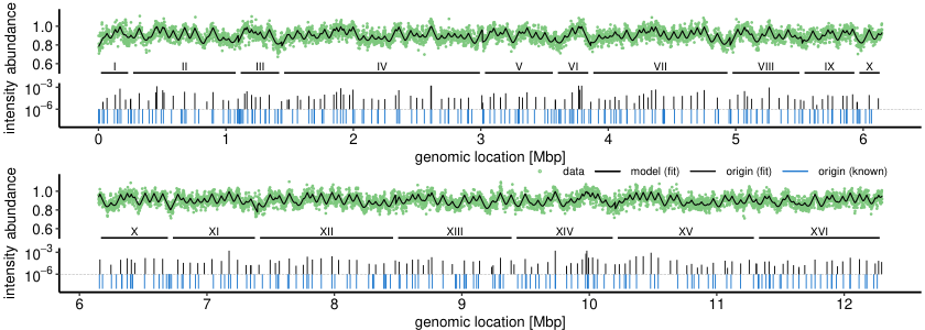
We now apply our model and inference procedure to experimentally measured DNA abundance in an asynchronous populations of budding yeast (S. cerevisiae W303) Müller et al. 2013. Our algorithm infers origins across the 16 yeast chromosomes. The predicted DNA abundance well matches the experimental one, see Fig. 5a.
Our method well predicts origins of replication with a resolution on the order of a few kilobases, and without using additional experimental information other than the DNA abundance distribution. The inferred origins locations correlate with known origins of S. cerevisiae when binned on a length scale of about 7kb, see Fig. 5b. A second correlation peak at 100kb suggests a large-scale pattern in the distribution of origins. As expected, the peak at 7kb vanishes when known origin locations are randomly shifted by , or shuffled by randomly reordering chromosomes. The results of the correlation analysis are corroborated by matching each inferred origin to the closed known origin (figure 5c; median distance 3.9kb) respectively each known origin to the closest inferred origin (figure 5d; median distance 6.6kb). In both cases, the average distances are significantly increased if the known origins are shifted or shuffled.
V Extensions of the theory
V.1 Non-exponential growth
Our approach can be generalized to populations that do not grow exponentially. We here assume that the number of genomes grows with time according to an arbitrary function . In this case, following the same logic of Section II, we find that Eq. (2) becomes
| (22) |
where . The proportionality constant can be determined by imposing normalization of . After integrating Eq. 22 by parts, we obtain
| (23) |
This generalization can be applied, for example, to bacterial or eukaryotic populations that grow in a partially synchronous manner. In such cases, might exhibit temporal peaks.
We note that, in Eqs. (22) and (23) we implicitly made the assumption that the replication program does not depend on . The validity of this assumption should be verified for populations that are out of steady growth. Moreover, a practical limiting factor can be the accuracy at which can be estimated.
V.2 Non-immortal genomes
For the purpose of computing the DNA abundance distribution, our assumption of immortal genomes is justified as long as typical genome lifetimes are much longer than the doubling time . This is usually a realistic assumption, but in some cases one may want to generalize our approach to include genome degradation. In such case, the exponential distribution in Eq. (2) should be replaced with the age distribution of surviving genomes. In particular, if genomes survive until age with probability , the age distribution is expressed by
| (24) |
up to a normalization constant.
V.3 Multiple genome types
The theory we developed so far applies to statistically identical genomes. This assumption is sometimes referred to as “identity at birth” in the literature on renewal processes Boldin et al. 2023: all genomes are born identical, and the differences that they might develop as they synthesize can be seen as independent outcomes of the same stochastic process.
There might be cases in which this assumption does not hold. For example, certain knockout mutations of E. coli lead to defective genome types that are inheritable Sinha et al. 2018. To address these scenarios, we extend our theory to cases in which different genome types coexist in the population, each characterized by a different replication program.
We call the number of genomes of type at time in the population, with . The total number of genomes is . Each genome of type can be replicated into a genome of type according a certain stochastic process. We assume that this stochastic process satisfies the Perron-Frobenius theorem, so that at long time the number of genomes are given by
| (25) |
Here is the leading eigenvalue of the dynamics, corresponding to the exponential growth rate of the population. The vector is the leading eigenvector, having non-negative real entries according to the Perron-Frobenius theorem, and normalized such that . The resulting replication program can then be obtained as an average over the genome types:
| (26) |
This average replication program can be substituted into Eq. (2) to determine the DNA abundance distribution.
V.4 Numerical simulations and analogy with stochastic resetting
The models we considered in Sections III and IV are analytically solvable. However, this might not be the case for more complex models. In this Section, we briefly present an interpretation of the DNA abundance distribution as the steady-state of a dynamical process implementing stochastic resetting Evans and Majumdar 2011; Evans et al. 2020. This analogy can be used for efficient numerical simulations.
The models introduced in Sections III and IV are described by linear equations. Formally, we assume that we can always write the stochastic process associated with a certain DNA replication program in terms of linear evolution operator , so that
| (27) |
We now introduce a modified version of this equation:
| (28) |
Equation 28 can be interpreted as describing a replication program equivalent to that of Eq. (27), but that is stochastically reset to its beginning at rate . Stochastic simulations of this process can be easily implemented numerically.
We note that is a steady solution of Eq. (28), i.e., it satisfies
| (29) |
This means that we can determine , up to an appropriate normalization constant, by sampling the stochastic dynamics described Eq. (28) at steady state. Such stochastic simulations can be efficiently implemented numerically Bhat et al. 2022.
VI Conclusions
In this paper, we introduced a general theory that connects the DNA replication program with the abundance of DNA fragments that one should expect in an asynchronously growing population of cells. Our theory builds on previous approaches Yoshikawa and Sueoka 1963; Sueoka and Yoshikawa 1965; Gispan et al. 2017; Bhat et al. 2022; Huang et al. 2022a and has the advantage of being based on a minimal set of realistic assumptions and allowing for stochastic replication programs. As we have demonstrated, these key properties make our theory applicable to a broad range of organisms, from bacteria to eukaryotes.
In the case of bacterial DNA replication, we proposed a model in which the replisome speed is modulated in time and replisomes can stochastically stall. We solved the model exactly and fitted its prediction against sequencing data of E.coli growing at different temperatures Bhat et al. 2022. The fits show that the period of speed oscillations matches the population doubling time, or equivalently the time interval between consecutive fork firing. Our model with time-periodic speed variations fits the data slightly better than the one with space-periodic variations as postulated in Bhat et al. 2022. Taken together, these observations support that the causes of oscillations are linked with the cell cycle, or alternatively with the fork firing rate. A possible candidate would be competition among multiple forks on the same genome Bhat et al. 2022. At variance with Ref. Bhat et al. 2022, the approach introduced in this paper leads to an analytical expression for the DNA abundance distribution, which considerably simplifies the inference procedure and provides additional physical insight.
The fits of the E.coli data reveal that the Peclet number characterizing the replisome dynamics is rather large. On the one hand, this observation confirms that simpler approaches that neglect stochasticity Huang et al. 2022b; Huang et al. 2022a provide reliable results, at least in the case of wild type E.coli. On the other hand, the diffusion constant, albeit small, provides important information about the uncertainty of the replisome meeting point. In E.coli, the Tus-Ter system is know to set bounds on the region in which replisomes can meet Elshenawy et al. 2015, thereby likely affecting this accuracy. It will be interesting for future studies to apply our approach to mutant strains, to see whether they are characterized by a different degree of uncertainty.
Stochasticity is definitely crucial in the eukaryotic case. We have used our approach to estimate the origins location and intensities for budding yeast from the DNA abundance distribution measured in Nieduszynski et al. 2006. Our approach is based on seminal work by Bechhoefer and coworkers Bechhoefer and Rhind 2012; Baker and Bechhoefer 2014, that we extended to asynchronously growing populations. A previous study Gispan et al. 2017 also attempted at extending the approach from Bechhoefer and Rhind 2012; Baker and Bechhoefer 2014 to asynchronously growing budding yeast. Our results differ from those of Ref. Gispan et al. 2017 in two different aspects. First, Ref. Gispan et al. 2017 assumed as a working hypothesis a uniform distribution for the distribution . In contrast, our central result in Section II shows that the distribution should be exponential under very general conditions. Second, in fitting the model to the data, Ref. Gispan et al. 2017 used experimental knowledge of the origin coordinates. Instead, our method was able to directly infer these coordinates, without requiring any additional experimental information other than the DNA abundance distribution.
In our eukaryotic model, we assumed for simplicity that replisome speed is constant; that origins are placed at well defined sites; and that they fire at an origin-dependent rate that is constant in time. The last assumption, in particular, is a drastic approximation, since origin firing rates in yeast are known to be markedly time-dependent Yang et al. 2010. Relaxing these assumptions constitutes an important challenge for future research and will permit to recover origin timing behaviour, beside locations, and thus provide a more complete picture of the replication program.
In any case, despite these simplifying assumptions, our algorithm successfully recovers the locations of the majority of known origins in budding yeast, with an accuracy on the order of kilobases. The accuracy can likely be further increased by exploiting advances in sequencing technology, in particular increased sequencing depth and read lengths, and by further improving the optimization algorithm. Our results demonstrate that the combination of deep sequencing of asynchronous populations and our inference approach provides a cost-effective way of discovering the replication origins of any single-cell eukaryotic species which can be cultured and sequenced.
Acknowledgements.
We thank S. Hauf, C. Plessy, and Y. Yokobayashi for fruitful discussions. We thank A. Alsina, J. Bechoefer, N. Rhind, P. Sartori, and A. Sassi for feedback on a preliminary manuscript. This work was supported by JSPS KAKENHI Grant No. 23H01146 (to SP). DB thanks Vellore Institute of Technology, Vellore for providing VIT SEED Grant-RGEMS Fund (SG20220060) for carrying out this research work.Appendix A Bacterial DNA replication with time-dependent speed
We consider the Langevin Eqs. (III.1). We write the associated Fokker-Planck equation for the first replisome:
| (30) |
Equation (30) shows that the function acts as global time rescaling. Therefore, if is a solution of the Fokker-Planck equation with constant drift and diffusion terms
| (31) |
under certain boundary and initial conditions, then
| (32) |
solves the original Fokker-Planck Eq. (30) with the same boundary and initial conditions, where . We impose, in particular, an absorbing boundary condition at , and an initial condition . The flux through the absorbing boundary is given by an inverse Gaussian distribution:
| (33) |
Since the first-passage density of Eq. (30) equals the flux , we have
| (34) |
The same approach can be used for the second replisome after a suitable change of coordinates and initial conditions. Integrating Eq. (34) over , and similarly for the second replisome, directly leads to Eqs. (III.1) and (III.1).
Appendix B Effect of diffusivity on the shape of the bacterial DNA abundance distribution
We here study the effect of increasing the diffusivity on the shape of the DNA abundance distribution . We first focus on the the meeting point region, and then consider the region far from the expected meeting point. We call the expected meeting point the “replication terminus”. Since this is the last location on the genome to be replicated, attains its global minimum there. For , exhibits a cusp at the terminus, and thus infinite curvature. For , the cusp vanishes, the curvature is finite and decreases with (Fig. 2c-d).
To quantitatively link with this curvature, we first use that Eq. (III.1) is symmetric under the swap of replisomes and mirroring of the genomic coordinate: . As a consequence, vanishes for all time and therefore according to Eq. 2. The curvature at is thus simply . We focus on the relative curvature expressed by
| (35) |
To make progress, we approximate the replication time distribution with a Gaussian:
| (36) |
where the mean and the variance have to be determined. It then follows from Eq. (3) that
| (37) |
Here, we have approximated the integral by extending the lower extreme to . We expect the error caused by this approximation to be negligible, since the Gaussian distribution that approximates must be concentrated on the positive real numbers. By using that and thus , and assuming that the dependence of on is small enough to be ignored, we obtain
| (38) |
We now have to evaluate . To make this tractable, we now further approximate the individual inverse Gaussian laws of , from Eq. (III.1) with Gaussian distributions. For these individual laws, the means and variances are given by Eq. (III.1) which yields
| (39) |
where we have for simplicity assumed that the replisome speed is constant, i.e. . Therefore:
| (40) |
and by inserting into Eq. (38) we obtain Eq. (11) for the normalized curvature of the DNA abundance at the terminus.
Eq. 37 also permits to approximate the value of itself at the terminus. We use that
| (41) |
and
| (42) |
Approximating and in Eq. (37) yields
| (43) | ||||
| close to the replication terminus. The curvature at is therefore | ||||
| (44) | ||||
We now study the shape of the DNA abundance far from the terminus region. Within these regions, only one of the two replisomes plays a relevant role. For simplicity, we focus on the region replicated by replisome 1. Also in this case, we assume constant replisome speed, i.e. . Since replisome 2 has virtually no chance of reaching the area of interest before replisome 1, we assume . The DNA abundance can then be explicitly found from the characteristic function of the inverse Gaussian distribution; the expansion yields for small
| (45) |
The change in the exponential decay rate due to is therefore of order .
Appendix C Uncertainty on the meeting point
We now consider the random point at which the two replisomes meet and its uncertainty . We call and the random times at which replisomes 1 and 2 reach location , respectively. Then, for all points to the left of the meeting point , and for all points to the right of . Therefore
| (46) |
We note that the means and variances in Eq. (III.1) are the means and variances of . Since increases monotonically, we substitute it into Eq. (46):
| (47) |
By using that and are independent, and substituting the means and variances from Eq. (III.1), we find the mean and variance of to be and , respectively. By approximating the distribution of the difference between the two replication times with a Gaussian, we obtain
| (48) |
where is the cumulative function of the Gaussian distribution. The uncertainly about the meeting point is therefore given by Eq. (12).
Appendix D Bacterial DNA replication with position-dependent speed
| [] | [] | [rad/Mbp] | [rad] | ||
|---|---|---|---|---|---|
| 17 | 230 22 | 1.0 1.2 | 0.18 0.07 | 6.2 6.7 | 2.3 1.6 |
| 22 | 350 37 | 1.0 1.6 | 0.23 0.15 | 2.8 0.73 | 3.4 0.72 |
| 27 | 540 17 | 0.4 0.5 | 0.18 0.04 | 4.6 0.11 | 2.1 0.11 |
| 32 | 820 57 | 1.4 2.3 | 0.12 0.04 | 5.5 0.13 | 1.6 0.16 |
| 37 | 970 25 | 2.9 2.3 | 0.18 0.02 | 4.3 0.15 | 3.0 0.14 |
(a) (b)
(a) (b)
In this Appendix, we solve a model with position-dependent speeds and in the limit of small diffusivity. This will allow us to directly compare time-dependent and position-dependent speed models. We allow the diffusion constants , to vary in space as well. The Langevin equations are:
| (49) |
where and . As in the case of Eq. (III.1), the initial conditions are , and we define replication programs , via the first-passage times of and , respectively, through position .
We now assume that (i) , change only slowly, (ii) , are small in comparison, and (iii) is not too close to the replication origin. Under these assumptions, replication times are approximately additive, meaning that if is the (random) time a replisome originating from takes to reach , then and are independent, and . For large enough , we invoke the central limit theorem for the sum and conclude that and are approximately Gaussian, implying
| (50) |
To find the position-dependent mean and variance , we rely on changing sufficiently slowly relative to so that we can find a subdivision where is approximately constant in each interval. By approximating the mean and variance of with the constant-speed solution, we obtain
| (51) |
We now compute and for the position-dependent speed fluctuations from Ref. Bhat et al. 2022 of the form
| (52) |
where is the distance of the replisome from the origin. We note that because we express in terms of distance travelled, the speed of the two replisomes when they traverse the same physical location will in general differ. Since integration of and is cumbersome, we first compute the following integrals of powers of , which are valid for :
| (53) | ||||
| We also introduce the definite integrals | ||||
| (54) | ||||
| Writing for the nearest integer we obtain | ||||
| (55) | ||||
and in terms of we finally have
| (56) |
By setting , and in Eq. (51) and inserting the means and variances into Eq. (50), we arrive at the replication program
| (57) |
Comparison of parameter estimates
Most parameter estimates for the position-dependent speed model obtained using the procedure outlined in Appendix E agree well with the values reported in Ref. Bhat et al. 2022, see Fig. 6a. Estimates that deviate also exhibit large uncertainties between replicates, see Table 2. These large uncertainties can be explained in a similar way as for the time-dependent model presented in Section III.
Parameter estimates also agree well between time- and position-modulated models, see Fig.6b. The oscillation frequency is not directly comparable between the two models, but when plotted against replication progress both models yield similar oscillations, see Fig. 7a. When the two models are compared across samples, we find that, for a large majority of samples, the time-dependent speed model yields a slightly higher likelihood than the position-dependent speed model, see Fig. 7b.
Appendix E Parameter estimation
(a)
(b)
(c)
 (d)
(d)
We compute the position-wise bias-corrected abundances and their uncertainties as
| (58) |
given the experimentally observed read counts at genomic locations in an exponentially growing () and stationary () populations Bhat et al. 2022. Since the counts and are typically large, we approximate the error distributions as Gaussian. Defining the parameter vector , we express the log likelihood by
| (59) |
where is a scaling factor.
We evaluate by a numerical integration of Eq.(3). This procedure requires a limited computational effort compared with Ref. Bhat et al. 2022, that evaluated the likelihood using stochastic simulations. We fit two different models corresponding to two different replication programs with are both instances of the general bacterial program from Eq. (7): (1) the time-dependent speed model in Eq. (III.1) with the modulating function given in Eq.(13). (2) the position-dependent speed model of Ref. Bhat et al. 2022 with replication program Eq. (57), see Appendix D (parameters are in this case, the parameter takes the place of ).
The likelihood surfaces of these models are quite rough, in particular with respect to and . This causes combined gradient-ascent optimization of all five parameters to remain stuck in local maxima, unless the initial estimate is close to the global optimum. On the other hand, exhaustive exploration of the parameter space for all 5 parameters at sufficient resolution is computationally expensive. We thus used the following procedure:
- 1.
We fit the constant-speed, no-diffusion (, ) regime by optimizing while keeping and . Initial value is .
- 2.
We fit the oscillatory no-diffusion (, ) regime by optimizing , , and while keeping . Initial values lie on a grid formed by the constant-speed, no-diffusion estimate of , , 25 logarithmically spaced values for from to ( being the genome length), and 5 uniformly spaced values for from to .
- 3.
We fit the constant-speed diffusive (, ) regime by optimizing and while keeping . Initial values lie on a grid formed by the constant-speed, no-diffusion estimate of , and 21 logarithmically spaced values for from to .
- 4.
We find the initial parameters for the oscillatory diffusive (, ) regime by optimizing , , and while fixing to the constant-speed diffusive estimate. Initial values are the same as in (2), except that for we now use the constant-speed diffusive estimate.
- 5.
We fit the oscillatory diffusive regime by optimizing , , , and , using the estimates found in (1)-(4) as initial values.
- 6.
We select the parameter regime with the lowest AIC score.
Identifiability
To study the identifiability of parameters , , , , of the bacterial replication program Eq. III.1 with we generated artificial DNA abundance distributions and estimated the parameters values using the procedure outlined in Appendix E. We randomly selected 2000 sets of parameters (Fig. 8a), and computed their predicted abundance profiles by simulating genomes using a fixed growth rate of ). We then generated Poisson-distributed read counts (and similarly for , using a flat abundance profile) from these abundance profiles, and ran the estimation procedure described in appendix E. All parameters except were recovered well (Fig. 8b).
Diffusivities below a certain value are unlikely to pass the Akaike information criterion and are therefore estimated to be zero. This occurs frequently for parameter sets corresponding to a Peclet number larger than 300 (Fig. 8c-d).
Appendix F Eukaryotic DNA replication
In this Appendix, we derive Eq. (21) for the DNA abundance in the case of origins at well-defined locations and with time-homogeneous firing rates, see Eq. (17). The general eukaryotic replication program is given by
| (60) |
see Bechhoefer and Rhind 2012; Baker and Bechhoefer 2014. Equation (60) is equivalent to Eq. (15), but with an explicit expression for the past light cone. We note that
| (61) |
We use Eq. (2) to obtain
| (62) |
Setting , i.e. assuming discrete origins , yields
| (63) |
and in the time homogeneous case we find
| (64) |
The integral can be then done by breaking it into different time intervals in which only a certain set of the theta functions are non-zero. This yields
| (65) |
where are the times it takes a replisome formed at the -th origin to reach position , and are ordered for g iven in such a way that . Therefore, we have
| (66) |
Equation (21) is obtained from Eq. (66) by substituting and as defined in Eqs. (19) and (20) and grouping terms with the same exponent.
Appendix G Eukaryotic origin inference by simulated annealing
We fit the solution of our eukaryotic model, Eq. (21), to experimentally measured DNA abundances in an exponentially growing asynchronous population of budding yest (S. cerevisiae W303)Müller et al. 2013. Also in this case, we correct for sequencing bias using the DNA abundance measured in a stationary population. Our input data are thus the ratios of number of reads in the exponential vs. stationary population found within each 1kb window along the W303 genome (GenBank accession CM007964.1). To estimate number and positions of origins and their fork firing rates, we use simulated annealing Bertsimas and Tsitsiklis 1993.
Our free parameters are the number of origins ; their positions and intensities , with ; and the ratio of growth rate to speed . We collectively refer to the vector of free parameters (excluding itself) as . To prevent over fitting, we use the Akaike information criterion (AIC) as the cost function, defined as
| (67) |
The first term on the right hand side of Eq. (67) penalizes a large number of origins, while the second term penalizes small log-likelihoods. The quantity is computed as in Eq. (59). The noise in the data appears larger than expected by Poissonian sampling. We therefore use the empirical noise estimate instead of the Poissonian error estimates from Eq. (58). Our estimate is based on the assumption that the systematic contribution to the quantity is negligible compared to the noise. We confirmed post-hoc this assumption by replacing the with the fitted model predictions. The resulting value is an order of magnitude smaller; therefore indeed mainly represents measurement errors rather than systematic effects.
Our simulated annealing algorithm comprises the following steps:
- 1.
We set the Monte-Carlo temperature to and generate an initial parameter vector . We draw uniformly from [, ] and place two origins randomly on each chromosomes with intensities drawn uniformly from [, ] .
- 2.
We generate a parameter proposal by executing one of the following moves with the indicated probability:
- •
Relocating an origin (prob. 24%). We choose one among the origins randomly and relocate it to a uniformly drawn position on the same chromosome. The origin firing rate remains unchanged.
- •
Altering one origin intensity (prob. 24%). We randomly choose one of the origins and replace its intensity rate with a value drawn uniformly from [, ] .
- •
Removing an origin (prob. 24%). We choose one among the origins and remove it unless it is the only origin on the chromosome.
- •
Adding an origin (prob. 24%). We add an origin at a uniformly drawn location on the genome with an intensity uniformly drawn from [, ] .
- •
Altering the growth rate (prob. 4%). We draw a new value of uniformly from [, ] .
The ranges of free parameters are chosen to cover replisome speeds () from to , doubling times between 50 minutes to 150 minutes, and fork firing delays between 1 minute and 150 minutes.
- •
- 3.
We accept with Metropolis probability
(68) - 4.
We reduce the Monte-Carlo temperature by a factor and reiterate from step (2). The total number of iterations is . With this choice, the final temperature is equal to .
After half the number of iterations (), the number of origins is already close to the final value (222 vs. the final number of 234), and repeating the procedure 10 times yield similar final numbers of origins (225 6). We take this as evidence that the algorithm has converged after iterations.
References
- Bechhoefer and Rhind (2012) J. Bechhoefer and N. Rhind, Replication timing and its emergence from stochastic processes, Trends in Genetics 28, 374 (2012).
- Baker et al. (2012) A. Baker, B. Audit, S.-H. Yang, J. Bechhoefer, A. Arneodo, et al., Inferring where and when replication initiates from genome-wide replication timing data, Physical review letters 108, 268101 (2012).
- Gispan et al. (2017) A. Gispan, M. Carmi, and N. Barkai, Model-based analysis of DNA replication profiles: predicting replication fork velocity and initiation rate by profiling free-cycling cells, Genome Research 27, 310 (2017).
- Hulke et al. (2020) M. L. Hulke, D. J. Massey, and A. Koren, Genomic methods for measuring DNA replication dynamics, Chromosome Research 28, 49 (2020).
- Xu and Dixon (2018) Z.-Q. Xu and N. E. Dixon, Bacterial replisomes, Current opinion in structural biology 53, 159 (2018).
- Gilbert (2001) D. M. Gilbert, Making sense of eukaryotic DNA replication origins, Science 294, 96 (2001).
- Costa and Diffley (2022) A. Costa and J. F. Diffley, The initiation of eukaryotic DNA replication, Annual Review of Biochemistry 91, 107 (2022).
- Yang et al. (2010) S. C.-H. Yang, N. Rhind, and J. Bechhoefer, Modeling genome-wide replication kinetics reveals a mechanism for regulation of replication timing, Molecular systems biology 6, 404 (2010).
- Rhind (2022) N. Rhind, DNA replication timing: Biochemical mechanisms and biological significance, BioEssays 44, 2200097 (2022).
- Cooper and Helmstetter (1968) S. Cooper and C. E. Helmstetter, Chromosome replication and the division cycle of Escherichia coli, Journal of Molecular Biology 31, 519 (1968).
- Fu et al. (2023) H. Fu, F. Xiao, and S. Jun, Bacterial replication initiation as precision control by protein counting, PRX Life 1, 013011 (2023).
- Berger and ten Wolde (2023) M. Berger and P. R. ten Wolde, Synchronous replication initiation of multiple origins, PRX Life 1, 013007 (2023).
- Raghuraman et al. (2001) M. K. Raghuraman, E. A. Winzeler, D. Collingwood, S. Hunt, L. Wodicka, A. Conway, D. J. Lockhart, R. W. Davis, B. J. Brewer, and W. L. Fangman, Replication dynamics of the yeast genome, science 294, 115 (2001).
- Daigaku et al. (2015) Y. Daigaku, A. Keszthelyi, C. A. Müller, I. Miyabe, T. Brooks, R. Retkute, M. Hubank, C. A. Nieduszynski, and A. M. Carr, A global profile of replicative polymerase usage, Nature structural & molecular biology 22, 192 (2015).
- Sueoka and Yoshikawa (1965) N. Sueoka and H. Yoshikawa, The chromosome of Bacillus subtilis. I. Theory of marker frequency analysis, Genetics 52, 747 (1965).
- Wendel et al. (2014) B. M. Wendel, C. T. Courcelle, and J. Courcelle, Completion of DNA replication in Escherichia coli, Proceedings of the National Academy of Sciences 111, 16454 (2014).
- Wendel et al. (2018) B. M. Wendel, J. M. Cole, C. T. Courcelle, and J. Courcelle, SbcC-SbcD and ExoI process convergent forks to complete chromosome replication, Proceedings of the National Academy of Sciences 115, 349 (2018).
- Midgley-Smith et al. (2018) S. L. Midgley-Smith, J. U. Dimude, T. Taylor, N. M. Forrester, A. L. Upton, R. G. Lloyd, and C. J. Rudolph, Chromosomal over-replication in Escherichia coli recG cells is triggered by replication fork fusion and amplified if replichore symmetry is disturbed, Nucleic acids research 46, 7701 (2018).
- Dimude et al. (2018) J. U. Dimude, M. Stein, E. E. Andrzejewska, M. S. Khalifa, A. Gajdosova, R. Retkute, O. Skovgaard, and C. J. Rudolph, Origins left, right, and centre: increasing the number of initiation sites in the Escherichia coli chromosome, Genes 9, 376 (2018).
- Rhind et al. (2010) N. Rhind, S. C.-H. Yang, and J. Bechhoefer, Reconciling stochastic origin firing with defined replication timing, Chromosome Research 18, 35 (2010).
- Bhat et al. (2022) D. Bhat, S. Hauf, C. Plessy, Y. Yokobayashi, and S. Pigolotti, Speed variations of bacterial replisomes, Elife 11, e75884 (2022).
- Huang et al. (2022a) D. Huang, A. E. Johnson, B. S. Sim, T. Lo, H. Merrikh, and P. A. Wiggins, The high-resolution in vivo measurement of replication fork velocity and pausing, Nature Communications 14, 1762 (2022a).
- Huang et al. (2022b) D. Huang, T. Lo, H. Merrikh, and P. A. Wiggins, Characterizing stochastic cell-cycle dynamics in exponential growth, Physical Review E 105, 014420 (2022b).
- Powell (1956) E. Powell, Growth rate and generation time of bacteria, with special reference to continuous culture, Microbiology 15, 492 (1956).
- Yoshikawa and Sueoka (1963) H. Yoshikawa and N. Sueoka, Sequential replication of Bacillus subtilis chromosome, I. Comparison of marker frequencies in exponential and stationary growth phases, Proceedings of the National Academy of Sciences 49, 559 (1963).
- Chandler and Pritchard (1975) M. Chandler and R. Pritchard, The effect of gene concentration and relative gene dosage on gene output in Escherichia coli, Molecular and General Genetics MGG 138, 127 (1975).
- Jafarpour et al. (2018) F. Jafarpour, C. S. Wright, H. Gudjonson, J. Riebling, E. Dawson, K. Lo, A. Fiebig, S. Crosson, A. R. Dinner, and S. Iyer-Biswas, Bridging the timescales of single-cell and population dynamics, Physical Review X 8, 021007 (2018).
- Morin et al. (2012) J. A. Morin, F. J. Cao, J. M. Lázaro, J. R. Arias-Gonzalez, J. M. Valpuesta, J. L. Carrascosa, M. Salas, and B. Ibarra, Active DNA unwinding dynamics during processive DNA replication, Proceedings of the National Academy of Sciences 109, 8115 (2012).
- Morin et al. (2015) J. A. Morin, F. J. Cao, J. M. Lázaro, J. R. Arias-Gonzalez, J. M. Valpuesta, J. L. Carrascosa, M. Salas, and B. Ibarra, Mechano-chemical kinetics of DNA replication: identification of the translocation step of a replicative DNA polymerase, Nucleic acids research 43, 3643 (2015).
- Jun et al. (2005) S. Jun, H. Zhang, and J. Bechhoefer, Nucleation and growth in one dimension. I. The generalized Kolmogorov-Johnson-Mehl-Avrami model, Physical Review E 71, 011908 (2005).
- Jun and Bechhoefer (2005) S. Jun and J. Bechhoefer, Nucleation and growth in one dimension. II. Application to DNA replication kinetics, Physical Review E 71, 011909 (2005).
- Kolmogorov (1937) A. Kolmogorov, Statistical theory of nucleation processes., Izu. Akad. Nauk SSSR 3, 355 (1937).
- William and Mehl (1939) J. William and R. Mehl, Reaction kinetics in processes of nucleation and growth, Trans. Metall. Soc. AIME 135, 416 (1939).
- Avrami (1939) M. Avrami, Kinetics of phase change. I General theory, The Journal of chemical physics 7, 1103 (1939).
- Sekimoto (1986) K. Sekimoto, Evolution of the domain structure during the nucleation-and-growth process with non-conserved order parameter, Physica A: Statistical Mechanics and its Applications 135, 328 (1986).
- Sekimoto (1991) K. Sekimoto, Evolution of the domain structure during the nucleation-and-growth process with non-conserved order parameter, International Journal of Modern Physics B 5, 1843 (1991).
- Baker and Bechhoefer (2014) A. Baker and J. Bechhoefer, Inferring the spatiotemporal DNA replication program from noisy data, Physical Review E 89, 032703 (2014).
- Müller et al. (2013) C. A. Müller, M. Hawkins, R. Retkute, S. Malla, R. Wilson, M. J. Blythe, R. Nakato, M. Komata, K. Shirahige, A. P. de Moura, and C. A. Nieduszynski, The dynamics of genome replication using deep sequencing, Nucleic Acids Research 42, e3 (2013).
- Shumate and Salzberg (2021) A. Shumate and S. L. Salzberg, Liftoff: accurate mapping of gene annotations, Bioinformatics 37, 1639 (2021).
- Boldin et al. (2023) B. Boldin, O. Diekmann, and J. Metz, Population growth in discrete time: a renewal equation oriented survey, arXiv preprint arXiv:2306.09193 (2023).
- Sinha et al. (2018) A. K. Sinha, C. Possoz, A. Durand, J.-M. Desfontaines, F.-X. Barre, D. R. Leach, and B. Michel, Broken replication forks trigger heritable DNA breaks in the terminus of a circular chromosome, PLoS genetics 14, e1007256 (2018).
- Evans and Majumdar (2011) M. R. Evans and S. N. Majumdar, Diffusion with stochastic resetting, Physical review letters 106, 160601 (2011).
- Evans et al. (2020) M. R. Evans, S. N. Majumdar, and G. Schehr, Stochastic resetting and applications, Journal of Physics A: Mathematical and Theoretical 53, 193001 (2020).
- Elshenawy et al. (2015) M. M. Elshenawy, S. Jergic, Z.-Q. Xu, M. A. Sobhy, M. Takahashi, A. J. Oakley, N. E. Dixon, and S. M. Hamdan, Replisome speed determines the efficiency of the Tus- Ter replication termination barrier, Nature 525, 394 (2015).
- Nieduszynski et al. (2006) C. A. Nieduszynski, Y. Knox, and A. D. Donaldson, Genome-wide identification of replication origins in yeast by comparative genomics, Genes & Development 20, 1874 (2006).
- Bertsimas and Tsitsiklis (1993) D. Bertsimas and J. Tsitsiklis, Simulated Annealing, Statistical Science 8, 10 (1993).