Electromagnetic Casimir-Polder Interaction for a Conducting Cone

The Casimir-Polder interaction between an uncharged conducting object on a polarizable particle Casimir and Polder 1948; Sukenik et al. 1993; Harber et al. 2005 provides one of the simplest examples of a mesoscopic fluctuation-based force. Since the particle can be treated as a delta-function potential, its effects can be evaluated in any basis. As a result, in the scattering formalism, the interaction energy between the particle and conducting object can be determined directly from the full electromagnetic Green’s function in the presence of the object. In contrast, for the Casimir force between two objects, one needs the scattering $T$-matrices for each object connected by the free Green’s function expressed in each object’s scattering basis to propagate fluctuations between objects Langbein 1974; Lambrecht et al. 2006; Emig et al. 2006; Kenneth and Klich 2006; Emig et al. 2007; Rahi et al. 2009.

Along with the standard plane, cylinder, and sphere geometries for which there exist analytic expressions in terms of scattering modes for the Green’s function in the presence of a perfect conductor, the conducting wedge Deutsch and Candelas 1979; Brevik and Lygren 1996, which also models a cosmic string Helliwell and Konkowski 1986, is a case where the Green’s function can be obtained analytically as a mode sum, by imposing the wedge boundary conditions through a discrete, fractional angular momentum index. However, one can also use analytic continuation to a continuous, complex angular momentum to express this Green’s function in terms of the $T$-matrix for scattering in the angular (rather than radial) variable Oberhettinger 1954; Carslaw 1914; Felsen 1957; Maghrebi et al. 2011, an approach that then extends to the case of the cone Maghrebi et al. 2011 and puts the Green’s function into a form that is more directly analogous to the sphere, cylinder, and plane results. Mathematically, this approach is based on the Mehler-Fock and Kontorovich-Lebedev transforms Yakubovich 1996. The complex angular momentum approach requires that we consider only imaginary frequencies, however, so while it is well-suited to equilibrium problems at both zero and nonzero temperature, it cannot be applied to heat transfer Krüger et al. 2012, which must be computed on the real axis.

All of these calculations allow for investigation of the Casimir-Polder interaction near a sharp edge or tip, where the derivative expansion approach Fosco et al. 2011; Bimonte et al. 2014; Bimonte et al. 2012a; Bimonte et al. 2016; Bimonte et al. 2012b is not applicable, yielding semi-analytic results in terms of a small number of integrals and sums. But this approach is limited to perfect conductors, and as a result complements calculations based on surface current methods Rodriguez et al. 2007; Reid et al. 2009; Reid et al. 2013; Bimonte and Emig 2021, which are more complex numerically but applicable to more general geometries and materials. Recent work using the multiple scattering surface method, in which one combines expansions in scattering between and within objects Emig and Bimonte 2023 provides a particularly relevant comparison by demonstrating the Casimir force between a dielectric wedge and plane.

Here we use the analytically continued scattering formalism to calculate the Casimir-Polder force of a conducting cone on a polarizable atom, as might arise, for example, in the case of a particle beam passing by an atomic force microscope. We begin by reviewing the wedge calculation in the discrete angular momentum approach, and show how to obtain the same result using the analytic continuation approach. We then extend this calculation to the case of the cone, obtaining a result in terms of a sum and integral over angular momentum variables. For the special case where the particle lies on the cone axis, the calculation simplifies to a single integral. This calculation can be straightforwardly extended to frequency-dependent polarizability and nonzero temperature, although in those cases an additional sum or integral over frequency must be done numerically.

We begin by reviewing the Casimir-Polder interaction energy for a conducting wedge, which was computed in Refs. Deutsch and Candelas 1979; Brevik et al. 1998 and considered in the context of repulsive forces in Refs. Milton et al. 2011; Milton et al. 2012. Let the wedge run parallel to the $z$-axis and have half-opening angle $0<\theta_{0}<\pi$ around $\theta=0$ with the wedge vertex located at $x=y=0$, and consider imaginary wavenumber $k=i\kappa$ with $\kappa>0$. Note that by allowing $\displaystyle\theta_{0}>\frac{\pi}{2}$, we will be able to consider the case where the particle is inside the wedge. For a particle located at angle $\theta\in[0,2\pi]$ obeying $\theta_{0}<\theta<2\pi-\theta_{0}$, one can write the full Green’s function for the wedge in terms of ordinary cylindrical wavefunctions of fractional order, Deutsch and Candelas 1979; Brevik and Lygren 1996

in terms of the magnetic (transverse electric) and electric (transverse magnetic) modes respectively,

with $\displaystyle p=\frac{\pi}{2(\pi-\theta_{0})}$, where the regular (outgoing) function is evaluated at the point $\bm{r}_{1}$ or $\bm{r}_{2}$ with the smaller (larger) value of the cylindrical radius $r$ and the radial functions are given in terms of Bessel functions for regular and outgoing modes as

This Green’s function then obeys

in the presence of the conducting wedge, while the free Green’s function $\mathfrak{G}_{0}(\bm{r}_{1},\bm{r}_{2},\kappa)$, given by setting $p=1$ and replacing the trigonometric functions $\sin(\ell p(\theta-\theta_{0}))$ and $\cos(\ell p(\theta-\theta_{0}))$ in Eq. (3) with $\displaystyle\frac{1}{\sqrt{2}}e^{i\ell\theta}$, obeys the same equation in empty space.

One can then use the “TGTG” Langbein 1974; Emig et al. 2006; Lambrecht et al. 2006; Kenneth and Klich 2006; Emig et al. 2007; Rahi et al. 2009 formulation of the Casimir energy, considering only the lowest-order interaction with the potential for a particle with polarizability ${\bm{\alpha}}$ at position $\bm{r}$,

which can be expressed in any basis since it is a delta-function. The result for the interaction energy of a particle with isotropic polarizability $\alpha$ becomes Deutsch and Candelas 1979; Brevik et al. 1998

where  Tr includes the trace over the spatial coordinate while  tr is the trace only over polarizations. In this approach, there is not a straightforward way to subtract the free contribution mode-by-mode, so one instead uses a point-splitting argument to subtract the entire contribution from the free Green’s function at once.

For the case of the cone, there does not exist an analog of this full Green’s function, written in terms of a rescaled order. As a result, we next recompute the result for the wedge using a different form of the Green’s function, which will generalize more readily to the case of the cone. In this approach, the angular momentum sum is replaced via analytic continuation by an integral, yielding for the free Green’s function Oberhettinger 1954; Maghrebi et al. 2011

where the transverse modes are

and we now take $\theta\in[-\pi,\pi]$. We have both even and odd modes, with regular modes given by

and outgoing modes given by

where the regular (outgoing) functions are evaluated at the point $\bm{r}_{1}$ or $\bm{r}_{2}$ with the smaller (larger) value of $|\theta|$. Note that the star indicates conjugation of the complex exponential part of the function only.

Although not needed for the computation, the corresponding longitudinal mode is

If its contribution is added to the free Green’s function, the result is equal to the scalar Green’s function
$\displaystyle\frac{1}{2\pi}\int_{-\infty}^{\infty}\frac{dk_{z}}{2\pi}K_{0}\left(\sqrt{\kappa^{2}+k_{z}^{2}}\left|r_{1}e^{i\theta_{1}}-r_{2}e^{i\theta_{2}}\right|\right)e^{ik_{z}(z_{>}-z_{<})}$ times the identity matrix; without this contribution, we obtain the same scalar times the projection matrix onto the transverse components. Here $z_{>}$ ($z_{<}$) is the $z$ coordinate associated with the point with the larger (smaller) value of $|\theta|$.

In this approach, we will take the wedge to be located at $\theta=\pm\theta_{0}$ and the particle’s location will always have $|\theta|>\theta_{0}$. We can then obtain the full Green’s function by replacing the regular solution with a combination of regular and outgoing solutions given in terms of the $T$-matrix

so that it now obeys the conducting boundary conditions on the wedge, yielding

In this form we can easily subtract the free Green’s function mode by mode, leaving only the terms with outgoing waves multiplied by the $T$-matrix. We obtain for the energy

where we have integrated over $\kappa$ and $k_{z}$ using polar coordinates. After carrying out the $\lambda$ integral, we obtain agreement with Eq. (9).

We now construct the Green’s function for the perfectly conducting cone with half-opening angle $0<\theta_{0}<\pi$, centered on the $z$-axis with the cone vertex at $z=0$, as shown in Fig. 1. We again consider imaginary wavenumber $k=i\kappa$ with $\kappa>0$. Note that by allowing $\displaystyle\theta_{0}>\frac{\pi}{2}$, we can consider the case where the particle is inside the cone. From Ref. Maghrebi et al. 2011, we have magnetic (transverse electric) and electric (transverse magnetic) transverse modes

with

where $P_{i\lambda-\frac{1}{2}}^{m}(\cos\theta)$ is the Legendre function of the first kind and $\displaystyle k_{i\lambda-\frac{1}{2}}(\kappa r)=\sqrt{\frac{2}{\pi\kappa r}}K_{i\lambda}(\kappa r)$ is the modified spherical Bessel function of the third kind, both with complex degree/order $\displaystyle\ell=i\lambda-\frac{1}{2}$. The “ghost” mode Maghrebi et al. 2011 is

where the $\pm$ sign is for regular and outgoing modes respectively. Its contribution arises from the contour integral used to turn the sum over the angular momentum quantum number $\ell$ into the integral over its analytic continuation $\lambda$, in which it cancels the contribution from the $\ell=0$ mode since that mode does not exist in electromagnetism. As a result, it is only ever evaluated at $\displaystyle\lambda=\frac{1}{2i}$, corresponding to $\ell=0$.

In this basis, the free Green’s function is Maghrebi et al. 2011

where the regular (outgoing) function is evaluated at the point $\bm{r}_{1}$ or $\bm{r}_{2}$ with the smaller (larger) value of $|\theta|$. Note that, as before, star indicates conjugation of the complex exponential part of the function only. Here the integral over $\displaystyle\lambda=\frac{1}{i}\left(\ell+\frac{1}{2}\right)$ represents the analytic continuation of the sum over $\ell$.

For completeness, we also give the longitudinal mode

for this geometry. If its contribution is added to the free Green’s function, the result is equal to the scalar Green’s function $\displaystyle\frac{\kappa}{4\pi}k_{0}\left(\kappa|\bm{r}_{1}-\bm{r}_{2}|\right)$ times the identity matrix; without this contribution we obtain the same scalar times the projection matrix onto the transverse components.

The full Green’s function in the presence of the conducting boundary $\mathfrak{G}$ is then given by the same expression with the replacement $\bm{\chi}^{\rm regular}{}^{*}\to\bm{\chi}^{\rm regular}{}^{*}+{\cal T}_{\lambda m}^{\chi}\bm{\chi}^{\rm outgoing}{}^{*}$, where $\bm{\chi}=\bm{M},\bm{N},\bm{R}$, again star indicates conjugation of the complex exponential part of the function only, and ${\cal T}_{\lambda m}^{\chi}$ is the corresponding $T$-matrix element Maghrebi et al. 2011

in terms of $\theta_{0}$, the half-opening angle of the cone. Subtracting the contribution from the free Green’s function then cancels the term with the regular solution, leaving only the product of outgoing solutions in the interaction energy.

After some algebra and simplification, we obtain the Casimir-Polder interaction energy for an atom with isotropic and frequency-independent polarizability $\alpha$ at distance $r$ from the cone vertex and angle $\theta$ from the cone axis, with $|\theta|>\theta_{0}$, as

where the last term arises from the “ghost” mode contribution. Here we have used Gradshteyn and Ryzhik 2007

to carry out the integral over $\kappa$, with integrals involving derivatives with respect to $r$ obtained by differentiating under the integral sign. The ghost term can be computed using the derivative of a geometric series,

along with an elementary $\kappa$ integral.

We can check this result numerically in the case of $\displaystyle\theta_{0}=\frac{\pi}{2}$, when it becomes the Casimir-Polder energy of a particle at a distance $d=r|\cos\theta|$ from a conducting plane, $\displaystyle U(\bm{r})=-\frac{3\alpha\hbar c}{8\pi d^{4}}$. We also note that we can simplify the difference of $T$-matrices to

by using the Wronskian relation between $P_{\ell}^{m}(z)$ and $P_{\ell}^{m}(-z)$.

Carefully taking the limit $\theta\to\pi$, we obtain the special case where the particle lies on the cone axis. Here the only contributions arise from $m=-1,0,+1$, leading to a result that simplifies to

for the cone-particle interaction energy when $\theta=\pi$. Here it is helpful to obtain the result in the first line, before integration over $\kappa$, because that result can straightforwardly be extended to nonzero temperature and frequency-dependent polarization, as will be described in more detail below.

Within this special case, it is illustrative to consider $\displaystyle\theta_{0}=\frac{\pi}{2}$, where the cone becomes a plane, for which we have ${\cal T}_{\lambda 0}^{N}=-1$ and $\displaystyle{\cal T}_{\lambda 1}^{N}=-{\cal T}_{\lambda 1}^{M}=-\frac{1}{\left(\lambda^{2}+\frac{1}{4}\right)}$. We can then use the $\kappa$ integrals above along with the integrals Gradshteyn and Ryzhik 2007; Oberhettinger and Higgins 1961¹¹ 1 The second integral does not appear to have been obtained previously.

where again integrals involving derivatives with respect to $r$ are obtained by differentiating under the integral sign, to do both the $\kappa$ and $\lambda$ integrals explicitly and in either order and obtain the standard results for the plane,

where in the second line we have done the $\lambda$ integral first, while in the third line we have done the $\kappa$ integral first. The former expression shows that if the ghost contribution is grouped with the electric modes, the contributions from the electric and magnetic modes match the planar calculation individually as functions of $\kappa$, and as a result reproduce the 5:1 ratio of their total contributions Milton 2019.

By repeating the above calculation in the case where $\alpha$ is a matrix, we can extend these results to the case of an anisotropic particle. We write the polarizability in the general form

where we have included both the symmetric and antisymmetric (nonreciprocal) off-diagonal components. Without loss of generality, we take the particle to be at $\phi=0$, so that it lies in the $xz$-plane. In terms of these parameters, we obtain for the energy

which on the axis $\theta=\pi$ simplifies to

Of particular interest is the $\gamma_{z}$ term, which generates a nonreciprocal torque around the $z$-axis. Comparing the $\alpha_{zz}$ and $\alpha_{\perp}$ contributions also enables us to compare whether a particle with a single polarization axis prefers to be aligned with or perpendicular to the axis of the cone.

To visualize these results numerically, in Fig. 2 we plot the Casimir-Polder interaction energy of an isotropic particle scaled by the fourth power of $r\sin(\theta-\theta_{0})$, which gives the perpendicular distance from the particle to the plane in the case where $\displaystyle\theta-\theta_{0}<\frac{\pi}{2}$. For $\displaystyle\theta_{0}=\frac{\pi}{2}$, the result in units of $\alpha\hbar c$ is $\displaystyle-\frac{3}{8\pi}\approx-0.1194$, and past this inflection point as the the cone envelops the particle, its interaction becomes much stronger.

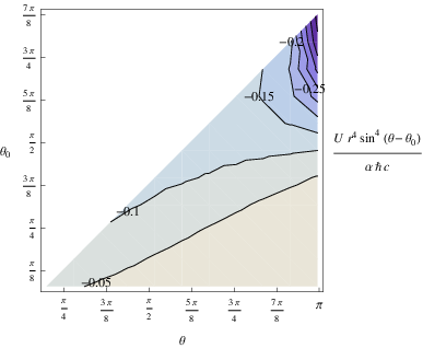
We note that all of these calculations can be extended to nonzero equilibrium temperature $T$, in which case the integral over $\kappa$ from $0$ to $\infty$ is replaced by $\displaystyle\frac{2\pi k_{B}T}{\hbar c}$ times the sum over Matsubara frequencies $\displaystyle\kappa_{n}=\frac{2\pi nk_{B}T}{\hbar c}$ for all $n=0,1,2,3,\ldots$, where the $n=0$ contribution is counted with a weight of $\displaystyle\frac{1}{2}$. This term must be considered carefully, since the Bessel function has a logarithmic singularity as $\kappa\to 0$ for fixed $\lambda$. For the special case of $\displaystyle\theta_{0}=\frac{\pi}{2}$, we can see explicitly from the above that this singularity disappears when the integral over $\lambda$ is done first, which should remain the case in general. In all of these calculations, one can also straightforwardly move $\alpha$ inside the $\kappa$ integral or sum to model a frequency-dependent polarizability. However, introducing either or both nonzero temperature and frequency-dependent polarizability then requires the $\kappa$ sum or integral to be carried out numerically.

It is a pleasure to thank M. Kardar for suggesting this problem and, along with K. Asheichyk, T. Emig, D. Gelbwaser, and M. Krüger, for helpful conversations and feedback. N. G. is supported in part by the National Science Foundation (NSF) through grant PHY-2209582.

References

- Casimir and Polder (1948) H. B. G. Casimir and D. Polder, Phys. Rev. 73, 360 (1948).
- Sukenik et al. (1993) C. I. Sukenik, M. G. Boshier, D. Cho, V. Sandoghdar, and E. A. Hinds, Phys. Rev. Lett. 70, 560 (1993).
- Harber et al. (2005) D. M. Harber, J. M. Obrecht, J. M. McGuirk, and E. A. Cornell, Phys. Rev. A 72, 033610 (2005).
- Langbein (1974) D. Langbein, Theory of Van der Waals Attraction (Springer-Verlag, Berlin, Heidelberg, 1974).
- Lambrecht et al. (2006) A. Lambrecht, P. A. Maia Neto, and S. Reynaud, New J. Phys. 8, 243 (2006).
- Emig et al. (2006) T. Emig, R. L. Jaffe, M. Kardar, and A. Scardicchio, Phys. Rev. Lett. 96, 080403 (2006).
- Kenneth and Klich (2006) O. Kenneth and I. Klich, Phys. Rev. Lett. 97, 160401 (2006).
- Emig et al. (2007) T. Emig, N. Graham, R. Jaffe, and M. Kardar, Phys. Rev. Lett. 99, 170403 (2007).
- Rahi et al. (2009) S. J. Rahi, T. Emig, N. Graham, R. L. Jaffe, and M. Kardar, Phys. Rev. D 80, 085021 (2009).
- Deutsch and Candelas (1979) D. Deutsch and P. Candelas, Phys. Rev. D 20, 3063 (1979).
- Brevik and Lygren (1996) I. Brevik and M. Lygren, Annals of Physics 251, 157 (1996).
- Helliwell and Konkowski (1986) T. M. Helliwell and D. A. Konkowski, Phys. Rev. D 34, 1918 (1986).
- Oberhettinger (1954) F. Oberhettinger, Communications on Pure and Applied Mathematics 7, 551 (1954).
- Carslaw (1914) H. S. Carslaw, Mathematische Annalen 75, 133 (1914).
- Felsen (1957) L. Felsen, IEEE Transactions on Antennas and Propagation 5, 121 (1957).
- Maghrebi et al. (2011) M. F. Maghrebi, S. J. Rahi, T. Emig, N. Graham, R. L. Jaffe, and M. Kardar, Proceedings of the National Academy of Sciences 108, 6867 (2011).
- Yakubovich (1996) S. B. Yakubovich, Index Transforms (World Scientific, 1996).
- Krüger et al. (2012) M. Krüger, G. Bimonte, T. Emig, and M. Kardar, Phys. Rev. B 86, 115423 (2012).
- Fosco et al. (2011) C. D. Fosco, F. C. Lombardo, and F. D. Mazzitelli, Phys. Rev. D 84, 105031 (2011).
- Bimonte et al. (2014) G. Bimonte, T. Emig, and M. Kardar, Phys. Rev. D 90, 081702 (2014).
- Bimonte et al. (2012a) G. Bimonte, T. Emig, R. L. Jaffe, and M. Kardar, EPL (Europhysics Letters) 97, 50001 (2012a).
- Bimonte et al. (2016) G. Bimonte, T. Emig, R. L. Jaffe, and M. Kardar, Phys. Rev. A 94, 022509 (2016).
- Bimonte et al. (2012b) G. Bimonte, T. Emig, and M. Kardar, Applied Phys. Lett. 100, 074110 (2012b).
- Rodriguez et al. (2007) A. Rodriguez, M. Ibanescu, D. Iannuzzi, J. D. Joannopoulos, and S. G. Johnson, Phys. Rev. A 76, 032106 (2007).
- Reid et al. (2009) M. T. H. Reid, A. W. Rodriguez, J. White, and S. G. Johnson, Phys. Rev. Lett. 103, 040401 (2009).
- Reid et al. (2013) M. T. H. Reid, J. White, and S. G. Johnson, Phys. Rev. A 88, 022514 (2013).
- Bimonte and Emig (2021) G. Bimonte and T. Emig, Universe 7, 225 (2021), ISSN 2218-1997.
- Emig and Bimonte (2023) T. Emig and G. Bimonte, Phys. Rev. Lett. 130, 200401 (2023).
- Brevik et al. (1998) I. Brevik, M. Lygren, and V. Marachevsky, Annals of Physics 267, 134 (1998).
- Milton et al. (2011) K. A. Milton, E. K. Abalo, P. Parashar, N. Pourtolami, I. Brevik, and S. Å. Ellingsen, Phys. Rev. A 83, 062507 (2011).
- Milton et al. (2012) K. A. Milton, E. K. Abalo, P. Parashar, N. Pourtolami, I. Brevik, and S. Å. Ellingsen, Journal of Physics A: Mathematical and Theoretical 45, 374006 (2012).
- Gradshteyn and Ryzhik (2007) I. S. Gradshteyn and I. M. Ryzhik, Table of Integrals, Series, and Products (Academic Press, San Diego, 2007), seventh ed.
- Oberhettinger and Higgins (1961) F. Oberhettinger and T. P. Higgins, Tables of Lebedev, Mehler and Generalized Mehler Transforms, no. 246 in Mathematical Note (Boeing Scientific Research Laboratories, Washington, 1961).
- Milton (2019) K. A. Milton, J. Opt. Soc. Am. B 36, C41 (2019).