Calculation of lepton magnetic moments in quantum electrodynamics: a justification of the flexible divergence elimination method

We work in the unit system where $\hbar=c=1$, the factors of $4\pi$ appear in the fine-structure constant: $\alpha=e^{2}/(4\pi)$, the tensor $g_{\mu\nu}$ corresponds to the signature $(+,-,-,-)$, the Dirac matrices satisfy the condition $\gamma_{\mu}\gamma_{\nu}+\gamma_{\nu}\gamma_{\mu}=2g_{\mu\nu}$. We also suppose $e=1$ for the lepton electric charge; since we work with each term of the perturbation series separately, it changes nothing, but makes the expressions shorter.

We extract the lepton AMM from QED Feynman graphs with $N_{l}=2$, $N_{\gamma}=1$, where by $N_{l}$ and $N_{\gamma}$ we denote the number of external lepton and photon lines in the graph; each graph may contain electron, muon, tau-lepton lines. We also assume that all graphs are one-particle irreducible and have no odd lepton loops (Furry’s theorem).

We work in the Feynman gauge with the propagators (1) for leptons and photons, respectively, where $m$ is the lepton mass.

There are the following types of UV-divergent subgraphs⁹⁹ 9 We consider only those subgraphs which are one-particle irreducible and contain all lines connecting the vertexes of the given subgraph; since odd lepton loops are forbidden, a UV-divergent subgraph is one-particle irreducible if and only if it is amputated. in QED Feynman graphs: lepton self-energy subgraphs ($N_{l}=2$, $N_{\gamma}=0$), vertexlike subgraphs ($N_{l}=2$, $N_{\gamma}=1$), photon self-energy subgraphs ($N_{l}=0$, $N_{\gamma}=2$), photon-photon scattering subgraphs¹⁰¹⁰ 10 Photon-photon scattering subgraph divergences cancel in the final result without subtraction, but they remain in the individual graphs. ($N_{l}=0$, $N_{\gamma}=4$).

Two subgraphs are said to overlap if they are not contained in each other and the intersection of their line sets is not empty.

A set of subgraphs of a graph is called a forest if any two elements of this set do not overlap.

For a vertexlike graph $G$, we denote by $\mathfrak{F}[G]$ the set of all forests $F$ consisting of UV-divergent subgraphs of $G$ and satisfying the condition $G\in F$. The lepton path of a graph $G$ connecting its external lepton lines is called the main path of $G$. By $\mathcal{I}[G]$ we denote¹¹¹¹ 11 The definition differs from that in Volkov 2016. the set of all vertexlike subgraphs of $G$ (including $G$) which have the vertex incident to the external photon of $G$ and at least one vertex of the main path of $G$.

To define the subtraction procedure, we use the linear operators labeled $A$, $U_{0},U_{1},U_{2},U_{3}$, $L$; sometimes the same names are used for operators applied to the Feynman amplitudes of subgraphs of different types. The definitions are:

• •

  $A$ is applied to vertexlike Feynman amplitudes¹²¹² 12 $p-\frac{q}{2}$, $p+\frac{q}{2}$ are incoming and outgoing lepton momenta, $q$ is the photon momentum. $\Gamma_{\mu}(p,q)$ and is defined as

  $$(A\Gamma)_{\mu}(p,q)=[A^{\prime}\Gamma]\gamma_{\mu},$$

  where $A^{\prime}$ is the projector of the AMM. See the definition of the projector in Volkov 2016; Volkov 2017.

• •

  $L$ is the standard on-shell renormalization operator for vertexlike graphs; it is defined as

  $$(L\Gamma)_{\mu}(p,q)=[L^{\prime}\Gamma]\gamma_{\mu},\quad L^{\prime}\Gamma=a(m^{2})+mb(m^{2})+m^{2}c(m^{2}),$$

  where

  $$\Gamma_{\mu}(p,0)=a(p^{2})\gamma_{\mu}+b(p^{2})p_{\mu}+c(p^{2})\not{p}p_{\mu}+d(p^{2})(\not{p}\gamma_{\mu}-\gamma_{\mu}\not{p}).$$

  (8)

• •

  $U_{0}$ is applied to photon self-energy and photon-photon scattering subgraphs and works as in standard renormalization. For the Feynman amplitude $\Pi_{\mu\nu}(p^{2})$ of the photon self-energy, we can take, for example,

  $$(U_{0}\Pi)_{\mu\nu}(p^{2})=[U_{0}^{\prime}\Pi][g_{\mu\nu},p^{2}g_{\mu\nu},p_{\mu}p_{\nu}],$$

  (9)

  where

  $$U_{0}^{\prime}\Pi=\left[h_{1}(0),\left.\frac{\partial h_{1}(p^{2})}{\partial p^{2}}\right|_{p^{2}=0},h_{2}(0)\right],$$

  (10)

  a scalar product is implied, and

  $$\Pi_{\mu\nu}(p^{2})=h_{1}(p^{2})g_{\mu\nu}+h_{2}(p^{2})p_{\mu}p_{\nu}.$$

  (11)

  Optimizations as described in Cvitanović and Kinoshita 1974b can also be used for photon self-energy graphs; the choice of the photon self-energy renormalization method does not play an important role in our subtraction procedure. For example, a more efficient method was used for the calculations; see Section V. However, the definition given here is convenient for proofs.

  For the Feynman amplitudes of photon-photon scattering, we can take

  $$(U_{0}\Pi)_{\mu_{1}\mu_{2}\mu_{3}\mu_{4}}(p_{1},p_{2},p_{3},p_{4})=\Pi_{\mu_{1}\mu_{2}\mu_{3}\mu_{4}}(0,0,0,0),$$

  where zero 4-momenta are denoted by $0$. It also can be defined with vector-valued operators $U_{0}^{\prime}$ as it was done for photon self-energy Feynman amplitudes.

• •

  $U_{j}$, $j=1,2$ are applied to vertexlike and lepton self-energy Feynman amplitudes; $U_{3}$ is applied only to vertexlike amplitudes. They are defined as

  $$(U_{j}\Gamma)_{\mu}(p,q)=[U_{j}^{\prime}\Gamma]\gamma_{\mu},$$

  $$(U_{j}\Sigma)(p)=M^{\prime}\Sigma+(U_{j}^{\prime}\Sigma)\times(\not{p}-m)$$

  (12)

  where $\Gamma_{\mu}(p,q)$ and $\Sigma(p)$ are vertexlike and lepton self-energy Feynman amplitudes, $U_{j}^{\prime}$ are number-valued linear operators,

  $$\Sigma(p)=r(p^{2})+s(p^{2})\not{p}.$$

  (13)

  $$M^{\prime}\Sigma=r(m^{2})+s(m^{2})m.$$

  (14)

  We require that:

  1. 1.

     $U_{j}$ ($j=1,2$) preserve the Ward identity: if $\Gamma_{\mu}$ and $\Sigma$ satisfy

     $$\Gamma_{\mu}(p,0)=-\frac{\partial\Sigma(p)}{\partial p^{\mu}},$$

     then

     $$(U_{j}\Gamma)_{\mu}(p,0)=-\frac{\partial[(U_{j}\Sigma)(p)]}{\partial p^{\mu}}$$

     is also satisfied. The latter can be rewritten as

     $$U_{j}^{\prime}\Gamma=-U_{j}^{\prime}\Sigma.$$

  2. 2.

     If $\Gamma_{\mu}(p,0)=0$, then $U^{\prime}_{j}\Gamma=0$ ($j=1,2,3$).

  We emphasize that the same symbol $U_{j}$ is used for lepton self-energy and vertexlike Feynman amplitudes; the definitions for the different types are independent from each other, the requirements connect them.

  These conditions are sufficient to prove combinatorially that the subtraction procedure defined below is equivalent to on-shell renormalization, provided that all regularization issues are resolved.

  To obtain finite integrals for each graph, more stringent requirements are needed. We take

  $$U_{j}^{\prime}\Gamma=a(M^{2}),\quad U_{j}^{\prime}\Sigma=-s(M^{2}),\quad j=1,2,$$

  where (8), (13) are satisfied, $M^{2}$ is an arbitrary real number (it may be different for different operators). As $U_{3}^{\prime}\Gamma$ we can take $a(M^{2})$ or $L^{\prime}\Gamma$.

  Being an operator means that it is applied to a function and depends only on this function (it does not depend on the internal structure of the corresponding subgraph). However, the same symbol $U_{j}$ is used for linear operators that are applied to Feynman amplitudes of different types (a type is the set of the external line types); the linear operators under the same symbol $U_{j}$ for different types can be chosen independently. Of course, $U_{j}$ can be chosen independently for different $j$. $U_{1}$ and $U_{3}$ are defined only for the Feynman amplitudes with the external leptons coinciding with those whose AMM is calculated; $U_{2}$ are defined for all types of external leptons (for example, it can be chosen independently for the Feynman amplitudes with external electrons, muons and tau-leptons).

The expression for the subtraction and extraction of the AMM corresponding to a Feynman graph $G$ is

where

here

the index of an operator denotes the subgraph to whose Feynman amplitude it is applied; $G_{1}\subset G_{2}$ or $G_{1}\subseteq G_{2}$ means $V(G_{1})\subset V(G_{2})$ or $V(G_{1})\subseteq V(G_{2})$, where $V(G)$ denotes the set of vertices of $G$. We emphasize that the whole graph $G$ is used in the definition of $\xi$; thus, $\xi$ does not depend on $G^{\prime}$ and $G^{\prime\prime}$. At the level of Feynman amplitudes, each term of the expression sequentially transforms the Feynman amplitudes of subgraphs using corresponding linear operators (the subgraphs should be ordered by inclusion in this sequence, from smaller to larger). Finally, the coefficient before $\gamma_{\mu}$ should be taken.

For example, for the graph $G$ from Fig. 1 the expression is

where $G_{e}=aa_{1}a_{2}b_{1}b_{2}c_{1}c_{2}c_{3}c_{4}d_{1}d_{2}d_{3}e_{1}e_{2}e_{3}e_{4}e_{5}$, $G_{d}=\{aa_{1}a_{2}b_{1}b_{2}c_{1}c_{2}c_{3}c_{4}d_{1}d_{2}d_{3}\}$, $G_{c}=aa_{1}a_{2}b_{1}b_{2}c_{1}c_{2}c_{3}c_{4}$, $\mathcal{I}[G]=\{G_{e},G\}$, subdiagrams are denoted by enumeration of their internal vertices; we should expand the parentheses to obtain the forest formula. The expression for this example does not depend on the type of leptons on the lepton loops ($U_{2}$ may be defined differently for different types of leptons, however).

Another example is the graph $G$ from Fig. 2. In this case, $\mathcal{I}[G]=\{G\}$, the expression is

The operator $U_{1}$ is applied to the subgraph $cdefghi$, because its external leptons are on the main path of $G$.

To obtain finite Feynman parametric integrals, all terms should be placed in the same Feynman parametric space. The algorithm for obtaining integrals from expressions is briefly explained in Volkov 2023 and in detail in Volkov 2016. The needed value of $A_{l}^{(2n)}$ is simply the sum of the integrals corresponding to the Feynman graphs involved.

The principle of divergence elimination in the method is similar to that explained in Volkov 2016 for the old method. Here we describe schematically how this choice of linear operators allows us to separate divergences and how it leads to divergence cancellation.

Let us consider the 1-loop unrenormalized vertexlike Feynman amplitude¹³¹³ 13 We ignore coefficients in this consideration.

Its IR-divergent part at $p^{2}=m^{2}$ is equal to

With

and the fact that $p_{\mu}$ commutes with all other multipliers that may appear in the expression, we obtain

where $A$ and $B$ some IR-divergent values¹⁴¹⁴ 14 We mean that a regularization is introduced, but we omit it for simplicity.. Thus, $U_{1}\Gamma_{1}$ and $U_{2}\Gamma_{1}$ are IR-finite. On the other hand, the UV-divergent part of $\Gamma_{1,\mu}(p,q)$ does not depend on $p,q$ and is therefore proportional to $\gamma_{\mu}$. Thus, $(L-U_{j})\Gamma_{1}$, $j=1,2$ are UV-finite.

There is a general observation:

• •

  $(L-U_{j})\Gamma$, $j=1,2,3$ has no overall UV divergence for any vertexlike Feynman amplitude $\Gamma$ (of any order);

• •

  $U_{j}\Gamma$, $j=1,2$ does not have IR divergences at all, provided that the mass renormalization has been done properly (see below);

• •

  this is also true for $U_{j}\Sigma$, $j=1,2$, where $\Sigma$ is a lepton self-energy Feynman amplitude.

In particular, this means that $U_{1},U_{2}$ can be used to subtract UV divergences without generating additional IR divergences (unlike $L$).

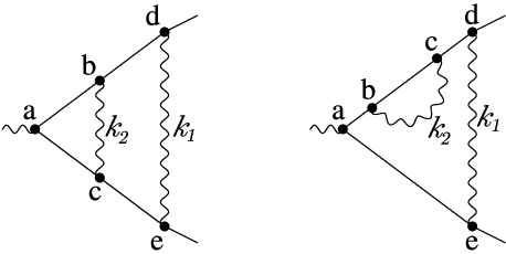
Consider the 2-loop ladder graph $G$ in Fig. 3,left¹⁵¹⁵ 15 Since changing the lepton line directions on a path or loop does not change the contribution, we will sometimes work with undirected Feynman graphs.. The corresponding expression is

In this case, we have only logarithmic divergences. The overall UV divergence corresponds to $k_{1},k_{2}\rightarrow\infty$; it is proportional to $\gamma_{\mu}$ and is cancelled in each term by $A$ or $L-U_{1}$. The overall IR divergence corresponds to $k_{1},k_{2}\rightarrow 0$. In all terms it is cancelled by $A$ since it is proportional to the Born amplitude $(A\gamma)_{\mu}=0$, where by $\gamma$ we denote the 4-vector of Dirac gamma matrices; this can be shown using standard methods for studying IR divergences in QED. There is also a mixed UV-IR divergence in this graph: $k_{1}\rightarrow 0,k_{2}\rightarrow\infty$; in this case, the UV divergence corresponding to $abc$ is IR-infinitely enhanced by the remaining propagators. In the first 2 terms it is cancelled by $A$, because the UV-divergent part of $abc$ is proportional to $\gamma_{\mu}$, so the “enhanced” value is proportional to $(A\gamma)_{\mu}=0$. In the remaining term, it is cancelled in $A_{abc}$ for the same reason. The remaining divergences¹⁶¹⁶ 16 This investigation is intended to demonstrate ideas only; a rigorous proof is not the goal in this case. are the UV divergence $k_{2}\rightarrow\infty$ and the IR divergence $k_{1}\rightarrow 0$. The first is cancelled in the sum of two terms by $1-U_{1}$ applied to the amplitude of $abc$ and in the last term by $A_{abc}$. The second does not exist in $A_{G}(U_{1})_{abc}$, in $A_{G}$ it enhances the amplitude generated by $A_{abc}$ by an IR-infinite multiplier, and it is cancelled by $(L-U_{1})_{G}A_{abc}$, because $L-U_{1}$ completely extracts the IR-divergent part of the enhancing multiplier.

Let us examine the graph $G$ on Fig. 3,right. The expression is

The difficulty in this case is the power-type IR-divergence corresponding to $k_{1}\rightarrow 0$ and a fixed $k_{2}\neq 0$. However, it is eliminated by the mass subtraction part in $U_{1}$. To make this possible, we give no freedom to the definition (14) of $M^{\prime}$ in (12). After the mass subtraction, the IR divergence becomes logarithmic and is removed by $A$, as is the overall UV divergence. The UV subdivergence of $bc$ is removed by $1-U_{1}$, and no additional IR divergence is generated.

Let us consider the graph $G$ on Fig. 4 . The expression is

The last multiplier eliminates the UV divergence corresponding to $fghi$; in this case there are no problems with IR divergences. The last term of the first multiplier removes the IR divergence corresponding to $k_{ae}\rightarrow 0$ (the subscript denotes the graph line by its ends). The term $A_{G}(U_{3})_{bcdfghi}$ removes the UV divergence corresponding to $bcdfghi$. It is important to note that it does not create any additional IR divergence, although $U_{3}$ has more freedom in definition than $U_{1}$ and $U_{2}$ (we can take $U_{3}=L$, for example). The reason is that the on-shell Feynman amplitude of $bcdfghi$ has no IR divergence, because its external photon is on a lepton loop.

The cancellation of divergences in Feynman parametric space for an arbitrary graph $G$ can be shown in a similar way as in Volkov 2016, but $U$ should be replaced everywhere by the corresponding $U_{j}$. Let us note one more small change. Following Volkov 2016, Appendix C, we assume that $G_{1}\subset\ldots\subset G_{n}\subset G_{n+1}=G$ are all elements of $\mathcal{I}[G]$. If $\xi=1$, where (15) is implied, we also assume that $G_{0}$ is the graph consisting of only one vertex of $G$ joining the external photon (if $\xi=3$, we use $G_{0}$ as the empty graph). By $z_{l}$ we denote the Feynman parameter corresponding to the internal line $l$. With the help of power counting, we investigate the case

where $\beta_{l}\geq 0$ are some numbers corresponding to the internal lines. By $P_{j}$ we denote¹⁷¹⁷ 17 In Volkov 2016 it is denoted by $P_{j}^{\prime}\cup P_{j}^{\prime\prime}$. the set of all lines $l$ on the main path of $G$ such that $l\in G_{j+1}$ and $l\notin G_{j}$. The cancellation of UV divergences and UV parts of mixed divergences is demonstrated in the same way¹⁸¹⁸ 18 The expression is organized in a very similar way to Zimmermann’s forest formula; this makes it possible to handle UV divergences. as in Volkov 2016. If all divergences not belonging to $\mathcal{I}[G]$ are properly subtracted, a potentially IR divergent case corresponds to a vector of divergences $[v_{0},\ldots,v_{n};w_{0},\ldots,w_{n}]$, where $v_{j}\geq w_{j}\geq 0$, $2v_{0}-w_{0}=2v_{1}-w_{1}=\ldots=2v_{n}-w_{n}>0$, there exists $j$ such that $w_{j}=0$. This vector gives the values

We will refer to the index $j$, $1\leq j\leq n$ as a transition index for the divergence vector $[v,w]$ if $v_{j}>v_{j-1}$. Correspondingly, the index $j$ is called an inverse transition index if $v_{j}<v_{j-1}$. The difference with the investigation in Volkov 2016 is the following:

1. 1.

   An index $j$ is called separating in a term of the expression if there is an operator $A_{G_{j}}$, $L_{G_{j}}$ or $(U_{3})_{G_{j}}$ ($U_{3}=L$) in this term. The difference with Volkov 2016 is the possibility to take $U_{3}$ (if it is equal to $L$).

2. 2.

   If $\xi=3$, then no consideration of the case $v_{0}>w_{0}$ is necessary; this case cannot produce divergence in a term, because $G_{1}$ has its external photon on a lepton loop.

3. 3.

   If $\xi=3$ and $U_{3}=L$, we rewrite the expression differently for a given index $H$ of the inverse transition in $[v,w]$:

   $$-\sum_{1\leq l<H}\left(L_{G}-(U_{1})_{G})(1-L_{G_{n}})\ldots(1-L_{G_{l+1}})A_{G_{l}}(1-L_{G_{l-1}})\ldots(1-L_{G_{1}})\right)$$

   $$+\sum_{H<l\leq n}\left((L_{G}-(U_{1})_{G})(1-L_{G_{n}})\ldots(1-L_{G_{l+1}})[L_{G_{l}}A_{G_{H}}-A_{G_{l}}](1-L_{G_{H-1}})\ldots(1-L_{G_{1}})\right)$$

   $$+[A_{G}-(L_{G}-(U_{1})_{G})A_{G_{H}}](1-L_{G_{H-1}})\ldots(1-L_{G_{1}})$$

   $$+\sum_{H<l\leq n}\left[\left(A_{G}(1-L_{G_{n}})\ldots(1-L_{G_{l+1}})-(L_{G}-(U_{1})_{G})\sum_{l<k\leq n}\left(A_{G_{k}}\prod_{\begin{subarray}{c}l<r\leq n\\ r\neq k\end{subarray}}(1-L_{G_{r}})\right)\right)\right.$$

   $$\times\left.\vphantom{\prod_{\begin{subarray}{c}l<r\leq n\\ r\neq k\end{subarray}}\left[\left(A_{G}(1-L_{G_{n}})\right)\right]}[L_{G_{l}}L_{G_{H}}-L_{G_{l}}](1-L_{G_{H-1}})\ldots(1-L_{G_{1}})\right].$$

   The last term was added to (C.7) in Volkov 2016, inappropriate $(1-U)$ multipliers were removed. The factor $L_{G_{l}}L_{G_{H}}-L_{G_{l}}$ cancels the divergence in this term, analogous to the other terms.

This argument shows how it works, but a full rigorous examination seems difficult and cumbersome; we rely on a numerical check (see Section V).