Linear stability of Poiseuille flow over a steady spanwise Stokes layer
Abstract
The temporal linear stability of plane Poiseuille flow modified by spanwise forcing applied at the walls is considered. The forcing consists of a stationary streamwise distribution of spanwise velocity that generates a steady transversal Stokes layer, known to reduce skin-friction drag in a turbulent flow with little energetic cost. A large numerical study is carried out, where the effects of both the physical and the discretization parameters are thoroughly explored, for three representative subcritical values of the Reynolds number . Results show that the spanwise Stokes layer significantly affects the linear stability of the system. For example, at the wall forcing is found to more than double the negative real part of the least-stable eigenvalue, and to decrease by nearly a factor of four the maximum transient growth of perturbation energy. These observations are -dependent and further improve at higher . Comments on the physical implications of the obtained results are provided, suggesting that spanwise forcing might be effective to obtain at the same time a delayed transition to turbulence and a reduced turbulent friction.
I Introduction
Decreasing the aerodynamic drag is a formidable scientific and technological challenge in configurations dominated by a relative motion between a solid body and a surrounding fluid. In particular, the skin-friction drag — in the laminar or in the turbulent regime — often represents a major portion of the total drag in the air transport sector, and can be of paramount importance in naval and submarine transport. Skin friction can be reduced either by keeping the flow laminar as long as possible, thus exploiting the intrinsically lower friction levels typical of the laminar regime, or by accepting the transition to turbulence, and reducing the level of turbulent friction below its natural level. A viable flow control approach that achieves both objectives would be very desirable, as it would first take advantage of laminarity as long as possible, and then continue to reduce turbulent friction.
Among the several active techniques for the reduction of turbulent drag, we are interested in spanwise-forcing techniques, and the present work in particular considers streamwise-traveling waves of spanwise wall-velocity as introduced by Quadrio et al. (2009) 1 1. Comprehensive reviews on this technique for turbulent drag reduction are available (2 2; 3 3; 4 4). The streamwise-traveling waves, which include as a special case the spanwise-oscillating wall (5 5) but achieve far higher energetic efficiency, abate the levels of turbulent skin-friction drag with interesting energetic effectiveness, with one energy unit spent on the control saving up to 30 units of pumping energy. Furthermore, recent evidence has shown that spanwise forcing can bring indirect benefits in terms of the reduction of pressure drag (6 6); in addition, it may be highly beneficial by interacting with the shock wave over an aerofoil in transonic flow (7 7) and reducing significantly the aerodynamic drag of the entire airplane with negligible energy expenditure. Within this context, the present work is motivated by the following simple question: Can spanwise forcing favorably affect transition to turbulence? Since the forcing is known to weaken near-wall streaks in a turbulent flow (8 8), a similar effect on laminar streaks might alter their growth, thus causing a delay of, or perhaps preventing altogether, transition to turbulence. It must be kept in mind that, at the moment, satisfactory actuators for implementing traveling waves in a real-world application are still lacking, even though some interesting developments exist, including mechanical movement of the wall (9 9; 10 10), electroactive polymers (11 11; 12 12) and the use of Kagome lattices (13 13). However, the prospect of instrumenting e.g. an airplane wing with one actuator that, in the wing fore part, would delay transition while, in the aft, would decrease turbulent skin-friction drag is certainly appealing, and motivates further research efforts into this direction.
This work is not the first to investigate the stability properties of a wall-bounded flow modified by spanwise forcing, and the available body of literature provides important guidance. Most of the current knowledge concerns spatially uniform wall oscillations. Jovanović (2008) 14 14 demonstrated the capability of properly designed wall oscillations to reduce receptivity of the linearized Navier–Stokes equations to small stochastic disturbances in laminar Poiseuille flow. Ricco (2011)15 15 showed in a linearized study that a substantial reduction in the intensity of laminar streaks under steady spatial oscillations is possible, with reductions up to 90% of the peak value of velocity fluctuations. Rabin et al. (2014) 16 16 studied plane Couette flow under spatially-uniform wall oscillations: by solving a fully non-linear problem, they demonstrated and quantified how the critical disturbance energy required for the onset of turbulence increases due to spanwise forcing. Hack et al. (2012) 17 17, using a linearized analysis of temporal harmonic wall oscillations, provided further evidence for near-wall shear filtering as an effective tool. In a follow-up study 18 18, the influence of spanwise forcing on by-pass transition in the boundary layer over a flat plate was examined. They found that oscillations, when properly tuned, can substantially delay transition, with overall energy gains. This DNS-based study was later corroborated by a corresponding Floquet stability analysis (19 19), where the changes in the linear modal and non-modal instability mechanisms operating in the pre-transitional boundary layer induced by the spanwise forcing were studied. This investigation confirmed important stabilization mechanisms due to weaker non-modal growth, but found that transition is enhanced, owing to a reinforcement of modal instabilities, at larger forcing amplitudes. Similarly, Wang et al. (2019) 20 20 found that spanwise oscillations of the wall can act as precursors to the transition process in a boundary layer.
For the spatially-varying case, where no stability study is presently available, Duque-Daza et al. (2012) 21 21 numerically solved a linearized version of the Navier–Stokes equations for a plane channel setting to investigate how streamwise-traveling waves impact the growth of near-wall low-speed streaks. They found that the computed relative change in streak amplification due to traveling waves varies with the parameters defining the wave in a way that strictly resembles the DNS-measured drag reduction data in the turbulent regime. Negi et al. (2015) 22 22 simulated via DNS a single low-speed streak forced by a standing wave of spanwise wall forcing in the laminar regime, and found that the skin friction can drop below the laminar reference value. They also reported a delay in the characteristic rise of skin friction during transition. Negi et al. (2019) 23 23 used LES to study bypass transition in a spatially evolving boundary layer. Temporal and spatial oscillations of the wall forcing were considered, and transition delay could be observed in both cases. A qualitative explanation was offered, attributing the transition delay to the additional filtering of the disturbance by the Stokes layer. An optimum forcing amplitude for transition delay was identified, while acknowledging that at larger wavelength the delay appears to increase monotonically with amplitude.
Motivated by the above studies, this work focuses on plane channel flow as a model problem and studies the modal and non-modal stability of the laminar, pressure-driven Poiseuille flow modified by streamwise-distributed spanwise forcing in the form of a steady Stokes layer, or SSL (24 24). The SSL is created by a (spanwise-uniform) stationary spanwise velocity at the wall that is sinusoidally distributed along the streamwise direction. The streamwise-varying base flow prohibits the direct application of a classic Orr–Sommerfeld–Squire (OSS) linear stability analysis, since the resulting system of differential equations contains streamwise-varying coefficients and thus requires a global approach. Here, extending an approach introduced by Floryan 25 25; 26 26, we exploit the particular form of the base flow to avoid a global stability analysis. The study is conceptually close to a classical secondary instability analysis, in which finite amplitude disturbances saturate and establish a new base flow, whose linear stability is then studied (27 27); in the present case, it is the superimposed sinusoidal spanwise flow that alters the Poiseuille streamwise base flow.
The structure of this paper is as follows. In §II the mathematical formulation is presented, emphasizing analogies and differences with respect to a classic OSS analysis; the numerical tools are validated against direct numerical simulations. Next in §III the physical parameters of the problem are discussed (the discussion of the discretization-related parameters is deferred to Appendix A), and the computational procedures employed in the execution of a large parameter study are described. In §IV the main results of the modal and non-modal stability analysis are discussed, and concluding remarks are offered in §V, together with a critical discussion of the main findings.
II Mathematical formulation
This section describes the setup of the linear stability analysis, based on the well-known Orr–Sommerfeld–Squire (OSS) problem for Poiseuille flow augmented by terms that model the presence of a spanwise base flow induced by the forcing.
The governing equations are the incompressible Navier–Stokes (NS) equations, which in non–dimensional form read:
| (1) |
where is the non-dimensional velocity field, is the non-dimensional pressure, and denotes the Reynolds number, defined with the kinematic viscosity of the fluid, the length scale in our case the channel half-height, and the velocity scale , in our case the centerline velocity of the laminar Poiseuille profile. The length and velocity scales and are used to express any quantity in dimensionless form. The NS equations are then expressed in a Cartesian coordinate system for the plane channel flow, with (and ) indicating the streamwise, wall-normal and spanwise directions (and corresponding velocity components). A sketch of the flow with the employed reference system is shown in Fig. 1.

The boundary conditions for the velocity at the wall are and , but, in contrast to standard Poiseuille flow, the spanwise component is non-zero. Within the general class of streamwise-traveling waves (1 1), the purely spatially modulated standing wave considered by Viotti et al. (2009) 24 24 is considered, so that the wall forcing applied at both walls is:
| (2) |
where denotes the maximum forcing amplitude, and stands for the forcing wavenumber.
II.1 The base flow
It was shown by Viotti et al. (2009) 24 24 (and later by Quadrio et al. (2011) 28 28 in the wider context of traveling-wave forcing) that in the laminar regime the spanwise wall-velocity does not affect the streamwise flow, which still follows the parabolic Poiseuille solution, but creates a wall-normal distribution of spanwise velocity. Hence, the base flow (indicated with an overbar) in the streamwise direction is identical to the no-forcing case , whereas the spanwise base flow , unaffected by the streamwise flow, corresponds to ; it is computed from the spanwise component of the momentum equation:
| (3) |
with the non-dimensional boundary condition
| (4) |
where is the imaginary unit. Equation (3) is linear with streamwise-constant coefficients. By enforcing periodicity and using separation of variables, the base flow has the form
| (5) |
where indicates the real part of a complex quantity, and the asterisk indicates complex conjugation. The function is computed numerically from the following parabolic cylinder equation, obtained by substituting (5) into (3) with :
| (6) |
Under the hypothesis that the thickness of the transverse Stokes layer is small compared to , and that streamwise diffusion is negligible with respect to the wall-normal diffusion, Viotti et al. (2009) 24 24 have determined the following solution:
in which Ai represents the Airy function (29 29), and is a representative wall-normal scale of the SSL, defined in terms of the fluid viscosity , the forcing wavenumber , and the longitudinal wall shear .
II.2 Linearized equations for the perturbations
Our interest lies on the dynamics of small perturbations to the base flow. After substituting the following decompositions:
| (7) |
into the NS equations (1), and subtracting the base flow equations from the linearized perturbation equations, obtained by dropping the quadratic terms in the small perturbations, one obtains
| (8) |
where the prime indicates the wall-normal derivative.
II.3 The formulation
The usual steps leading to the OSS equations (27 27) can be followed here to obtain a compact expression of the linear dynamics, under the incompressibility constraint, in terms of two evolution equations for the wall-normal components and of the perturbation velocity and vorticity vectors, respectively. The former equation reads
| (9) |
while the latter equation can be stated as
| (10) |
with boundary conditions of the form
| (11) |
As in the standard case, these two equations are complemented by a differential system which relates and to and via the continuity equation and the definition of the wall-normal vorticity. In contrast to the no-forcing OSS case, the two equations are fully coupled via , and several coefficients are varying along the streamwise direction.
II.4 Fourier transform
The standard OSS system is conveniently Fourier-transformed along the two homogeneous wall-parallel directions. In our case, this step can be straightforwardly applied in the spanwise -direction, giving rise to an expansion with spanwise wavenumber , since equations (9) and (10) consist of -independent coefficients. The coefficients’ streamwise dependence in equations (9) and (10) prevents a straightforward Fourier transform in that direction. However, their functional variation is not generic, as it derives from the functional form of the base flow (5) only; hence the coefficients must be harmonic functions of with wavenumber . We follow an approach introduced in Ref. 25 25 for the study of the stability of a parallel wall flow modified by periodic blowing and suction, and leverage the sinusoidal variation of the base flow. The flow variables are expanded in a (finite) Fourier series along the streamwise direction as:
| (12) |
with as the degree of the spectral expansion of the flow variables, as an integer index, and as a real number defining the actual expansion wavenumber . The parameter is referred to as the detuning parameter, since it is used to detune the perturbation against the base flow. In this preliminary work, we set . Note that Ref. 25 25 considered , whereas in this work is much larger and, like the other discretization parameters, is dynamically adapted to each case after a sensitivity analysis. The procedure for setting the discretization parameters is described in Appendix A.
Equations (9) and (10) can now be Fourier-transformed along the -direction, introducing the streamwise wavenumber in the process. A generic -dependent term is Fourier-transformed as follows:
Since in equations (9) and (10) terms with complex exponentials are of the kind and , Fourier-transforming in the -direction leads to integrals of the following general form:
Owing to the orthogonality of the trigonometric functions, they are proportional to , i.e. they are always zero unless . By introducing the operator , the equation governing the evolution of is
| (13) |
Analogously, the equation for reads
| (14) |
where .
When compared to the standard OSS problem, equations (13) and (14) contain several additional terms related to the spanwise base flow, described by the function . Terms containing and evaluated at are identical to the OSS equations, whereas the remaining terms represent effects of disturbances at wavenumbers .
II.5 Numerical discretization
From here on, a change in notation is introduced. In fact, the governing equations (13) and (14) can be equivalently derived by substituting the modal expansions (12) into the – equations and by Fourier-transforming against a testing function of the form , where is an integer such that .
Starting from this form, the -dependent terms are discretized via Chebyshev polynomials on a grid of Gauss-Lobatto nodes (30 30; 31 31; 32 32). The unknown is thus written as:
| (15) |
or, in matrix form, , with as a square matrix. Similar matrices , and represent the first, second and fourth derivative.
For a given , equations (13) and (14) can be written compactly in the following block form:
| (16) |
where is a diagonal matrix, describes the interaction of and , for a given wavenumber , with themselves (red blocks in Fig.2); and (green and yellow blocks in Fig.2) describe the interactions with the previous and subsequent streamwise wavenumbers, respectively, and contain the effect of the spanwise base flow.

Equation (16) must be solved for all of the truncated modal expansion . Therefore, after grouping the unknowns and into a single array of unknowns q, one obtains the following block form:
| (17) |
where q is a vector composed of pairs of – components, each at a different value, so with dimension ; and are block-tridiagonal square matrices, whose dimensions are . The structure of the system matrix is shown in Fig.2, which emphasizes its block-tridiagonal structure, with block size .
The boundary conditions (11) at the two walls are rewritten as:
| (18) |
They are readily enforced via appropriate modifications of the matrices , , and . Following Ref. 27 27, the boundary values for and are set not to exact zero, but to a very small value, i.e. ; the extremely fast dynamics associated to this non-zero values does not interfere with the flow dynamics, but the accuracy in computing eigenvalues is improved as the spurious modes associated to the discrete boundary condition are mapped far away in the complex plane.
II.6 Modal and non-modal stability characteristics
In what follows, the modal stability of the system will be assessed by computing the eigenvalues of the system matrix which describes the linearized dynamics of the system. Due to the size and sparsity of the matrix, its eigenvalues are most efficiently computed with the Arnoldi method (33 33). The number of eigenvalues totals , but only a modest fraction of them is of interest here, hence only a subset is computed. This is achieved by a truncation operator T, a matrix with dimensions . The relation transforms equation (17) as
| (19) |
where is a diagonal matrix containing the computed eigenvalues and T contains the corresponding eigenvectors.
While computing the largest eigenvalue would in principle suffice for deciding on modal stability or instability, choosing the right size of the truncation operator is essential to studying the non-modal stability of the flow (see e.g. Refs. 34 34; 27 27; 35 35). The kinetic energy density of an infinitesimal perturbation for a given is written as
| (20) |
with ; the superscript stands for Hermitian, i.e., the complex conjugate transpose.
After a Chebyshev expansion of and after computing the integral weights using the Clenshaw-Curtis quadrature formula (36 36; 37 37; 38 38; 39 39), one obtains
| (21) |
where W is a diagonal matrix containing the integral weights, and represents the energy weight matrix.
Once the full modal expansion is considered, the square of the energy norm of q becomes:
where is the block-diagonal positive definite energy weight matrix for all indices in the modal expansion. The energy norm can be rewritten using the truncation operator T:
where can be further decomposed via a Cholesky decomposition to result in
The transient energy growth eventually becomes
| (22) |
Lastly, the spatial shape of the optimal perturbation , and the corresponding spatial shape at the time of the largest energy growth , are given by:
| (23) |
where and are the first right and left singular vectors of the matrix , respectively.
II.7 Validation
The MATLAB numerical toolkit developed for the stability analysis is first validated against the results of a non-linear DNS solver. The code, introduced in Ref. 40 40, where full details are available, solves the incompressible Navier–Stokes equations with mixed spatial discretization, with Fourier expansions in the homogeneous directions (where the pseudo-spectral approach is used) and compact, fourth-order explicit finite-difference schemes in the wall-normal direction.
The transient energy growth function computed by the stability code is compared with the DNS-computed temporal evolution of the energy of the optimal initial condition. The test is carried out for , , . According to the discretization criteria described later in Sec.III and Appendix A, the discretization parameters are set to , and or . The DNS is carried out with 101 points in the wall-normal direction, Fourier modes in the streamwise direction, and 16 modes in the spanwise direction; the size of the temporal step is computed via the Courant-Friedrich-Lewy (CFL) condition, by enforcing ; it is verified that the outcome of the DNS is insensitive to further refinements in the temporal and/or spatial discretizations. The initial field for the DNS is made by the base flow, to which the optimal initial condition obtained by the non-modal stability code is added, after rescaling the amplitude to remain within the limits of linearity. Figure 3 compares the temporal history of the DNS-computed energy with the transient growth function for the uncontrolled and controlled cases. It can be observed that, as required by their definition, at all times; the two functions coincide at time . The controlled case with this particular choice of parameters exhibits a reduced maximum transient growth.
III Parameters and computational procedures
The present multi-parameter study considers the effects of the following nine parameters, either physical or related to the discretization of the problem:
- 1.
, the Reynolds number of the flow;
- 2.
, the maximum amplitude of the wall forcing in equation (2);
- 3.
, the streamwise wavenumber of the wall forcing in equation (2);
- 4.
, the spanwise wavenumber of the perturbation;
- 5.
, the number of Chebyshev polynomials in equation (15)
- 6.
, the truncation factor in the modal expansion (12)
- 7.
, the number of eigenvalues retained in the Arnoldi algorithm after truncation;
- 8.
, the temporal step for the discrete evaluation of ;
- 9.
, the time at which the computation of is stopped.
The first four parameters listed above are of a physical nature, and their range defines the breadth of the study. The remaining parameters are discretization parameters which impact the reliability of the results and the computational cost of the study. The vast range of explored physical parameters, together with the anticipated variable behavior of the system within it, requires efficiency and sensitivity considerations with regard to the chosen discretization.
Description of the choice of the discretization parameters is deferred to Appendix A. As far as the physical parameters are concerned, only three subcritical values of the Reynolds number are considered in this study, namely , and . The wall forcing is defined by two parameters: its dimensionless amplitude is varied between 0 and 1 in increments of 0.1 (resulting in 11 values), and its dimensionless wavenumber is varied between 0.5 and 5 in increments of 0.25 (yielding 19 values). The spanwise wavenumber is varied between 0 and 5, with 18 non-equispaced values specifically selected to focus on the most interesting regions. Note that corresponds to the most unstable two-dimensional waves predicted by the modal theory. implies a maximum spanwise velocity equal to the centerline Poiseuille velocity, and implies a forcing wavelength that is times the channel heigth. Overall, 11,286 cases are computed. The total computational cost is thus considerable, and exceeds 10000 core hours; a workstation equipped with an Intel i7 CPU with 6 cores has been used.
IV Results
IV.1 Modal stability
The modal stability characteristics of the flow are evaluated in terms of the real part of the least stable eigenvalue of the system matrix . The effect of wall forcing, represented through the physical parameters , , and , on the modal stability properties is quantified via the attenuation-rate increase, expressed via the ratio , defined as:
where is the least-stable eigenvalue of the unforced Poiseuille flow. Since the considered -numbers are subcritical, , and a positive effect of the forcing in the direction of increased stability margin implies , in analogy with the drag reduction rate used in the turbulent case to assess the effectiveness of the forcing. The discretization parameters are set according to the criteria described in Appendix A.
| 500 | 2.25 | 0.7 | 1 | 1.9380 |
| 1000 | 2.00 | 0.5 | 1 | 2.1725 |
| 2000 | 3.00 | 0.5 | 1 | 2.3636 |
For the various values of , table 1 reports the values of , and which have been found to yield the largest increase of . The results are -dependent, with going from at ( decreases from -0.00591 to -0.01146) to at ( decreases from -0.00135 to -0.00321). The stabilizing effect of spanwise forcing is significant, since at the negative real part of the least-stable eigenvalue increases (in absolute value) by more than 2.3 times. It should come as no surprise that the effectiveness of the forcing depends on its amplitude : indeed, in table 1 the largest are consistently obtained for the largest forcing amplitude tested, i.e. . Once the optimal values of and are determined, figure 4 depicts how changes as a function of . For all Reynolds number studied, is quite similar to the turbulent drag reduction rate, and exhibits a monotonic growth from the uncontrolled case with , then saturating at large amplitudes. Especially at higher , the effect of forcing is already noticeable at rather small forcing intensity: for example, at a forcing with provides more than 85% of the benefit achievable at . This observation is important in view of the rapid increase of the energetic cost of the forcing.

To examine how the results depend on , we first observe that, in table 1, the optimal does not vary much with . Indeed, the optimum with respect to is rather flat. As an example, at figure 5 plots in --planes taken at three selected values of , namely , and . The plot demonstrates the weak dependence of on the forcing wavenumber, especially in the vicinity of the optimum value .
IV.2 Non-modal stability
| 500 | 1.25 | 1.5 | 1 | 2.8877 |
| 1000 | 0.75 | 2.5 | 1 | 3.3670 |
| 2000 | 0.75 | 1.5 | 1 | 3.6140 |
To shed light on the forcing-induced modifications to the short-term stability properties of the flow, we now proceed to consider the transient growth function and its maximum . is the maximum possible relative amplification of the initial perturbation energy, occurring at time for a specific initial condition referred to as the optimal input. We quantify the effect of the forcing on the non-modal stability by computing the ratio defined as:
where is the maximum transient growth for the reference Poiseuille flow. As in the modal analysis, the discretization parameters are set according to the criteria discussed in Appendix A. Table 2 presents the optimal parameters , and which have been found to provide the largest . As for modal stability, changes in are Reynolds-number-dependent, and the maximum reduction of the transient energy growth ranges from at (with decreasing from 43.39 to 15.03) to at (with decreasing from 689.52 to 190.80).
At the optimal values reported in table 2, the transient energy growth with and without forcing is compared in figure 6 (left). The transient growth is clearly inhibited by the spanwise forcing, and indeed the maximum energy amplification decreases from about 700 times the initial energy to less than 200 times; moreover, the maximum amplification occurs at an earlier time. At least for this specific case, for the forced case is above the reference curve for very short times.
The role of the two parameters and defining the wall forcing, is similar to the one discussed previously for modal stability. The forcing amplitude directly affects the amount of transient growth reduction, as clearly shown in figure 6 (right), while the forcing wavenumber has a lesser effect: as the wavenumber exceeds the optimal values identified in table 2 (which are close to the minimum value of considered in the present study), the effectiveness of the forcing does not exhibit a significant or rapid decrease.
Nonmodal stability theory readily provides access to the shape of the perturbation that triggers the maximum transient energy growth. The optimal input (and the corresponding optimal output), discussed in section II and obtained by means of a singular values decomposition, are examined in physical space in figures 7 and 8.
In particular, figure 7 describes how the optimal initial condition is affected by the forcing. The top row refers to the reference case with and confirms that, for plane Poiseuille flow, the optimal initial condition is a streamwise-constant pair of large-scale space-filling rolls. Indeed, in Fourier space such a perturbation is fully represented by the mode , leading to an effective streamwise wavenumber . When the spanwise forcing is active with (bottom row), the optimal initial condition is characterized by different streamwise wavenumbers. In particular, the morphology of the streamwise component of the optimal initial condition reveals the fundamental mode of the forcing, with superimposed higher harmonics. A striking difference to the unforced case is that the -component, although not entirely two-dimensional, is predominantly structured along the spanwise direction, i.e. orthogonal to the unforced case. Another significant difference is the fact that the perturbation becomes highly localized near the wall, and remains confined within the high-shear region produced by the spanwise Stokes layer described by the base flow. Though barely visible at this , a streamwise modulation can be observed in the spanwise component as well, whose overall shape however still resembles very much that of the unforced flow. The vertical component appears to be essentially unaffected by the forcing. In terms of relative intensity, the three velocity components are comparable with/without control; while the amplitudes of the wall-normal and spanwise components are unchanged, that of the longitudinal component, which is the smallest, grows by about six times in the controlled case.


If attention is drawn to the temporal evolution of the optimal initial condition, shown in figure 8 at the time of maximum energy amplification, similar effects are evident regarding its spatial shape; the spanwise forcing at the wall introduces a streamwise modulation with higher harmonic components. The modulation is however more reduced in comparison to the initial condition, and – at least for the case under consideration – it appears that at the perturbation has developed the same qualitative shape in both cases. The reorientation of the -component from the spanwise to the streamwise direction is attributed to an Orr-type mechanism (41 41): the initial disturbance is characterized by a flow pattern opposed to the mean shear which, as time evolves, is tilted into the shear direction.
To explain how the transient growth is altered, one has to consider the energy levels of the perturbation. Within the present linear setting the absolute value of the perturbation amplitude is inconsequential, and perturbations are normalized to unit maximum absolute value. However, the relative values of the various components and their growth rates can be informative. In the reference flow, the three velocity components of the initial condition at are relatively balanced, but the transient growth affects them very differently. In fact, the relative increment of the amplitude of the streamwise component is 481 times the initial value (this figure is obviously -number-dependent), whereas the and components decrease by factors of 0.47 and 0.46, respectively. With spanwise forcing, however, the picture is drastically changed. The evolution of the - and -components is similar to the unforced case, as they reduce to 0.51 and 0.46 of their initial value for and respectively. However, the growth of the streamwise component is severely inhibited, and at the increase of the streamwise velocity component is only 44 times, instead of 481 times.
IV.3 Discussion
The largest and identified in this study correspond to the best performance observed in the parameter space (, , ) for a given . However, it is important to realize that the amplitude and wavenumber are indeed specifiable parameters of the forcing, but the spanwise wavenumber of the perturbation, describing a generic small disturbance, is not a control parameter. Furthermore, background disturbances are realistically assumed to contain all frequencies. Hence, to appreciate the true potential of spanwise forcing, one should compare the neutral curve of the unmanipulated Poiseuille flow with a neutral curve for the controlled Poiseuille flow, where all values of are considered and the worst-case scenario is selected. This is shown in figure 9 (left), where a forcing defined by and is selected from the optimal parameters identified above. For the neutral curve we scan through from 5750 to 5850 by increments of 5, and through the wavenumber from 0.8 to 1.2 by increments of 0.05. Every point in the - plane for the forced flow results from a scan over all available spanwise wavenumbers . For the unforced flow the critical value of the Reynolds number is the well-known ; for , this threshold is increased, but only marginally so, to . The increment is not particularly relevant, in contrast to the optimal situation discussed above in IV.1. In line with the minimal change of , the shape of the most unstable eigenmode, i.e. the linearly unstable Tollmien–Schlichting wave, is also not altered significantly by the forcing. This means that the spanwise forcing is indeed capable of hindering the growth of certain spanwise perturbations, but not of all of them. Once the global effect of the forcing is considered in a scenario where perturbations of any wavenumber are present, the improvement is significantly smaller.
However, in the context of highly subcritical flows the significance of this result is limited, since the non-modal stability characteristics are way more important. With non-modal stability, the overall picture improves substantially. The maximum transient growth is significantly inhibited by spanwise forcing, regardless of the considered perturbation. As shown in table 2, the ratio increases from at to at . Following the discussion above, it is interesting to assess how the forcing improves the stability characteristics by finding the value of which yields the minimum . Figure 9 (right) plots how depends on , at and for the three Reynolds numbers, after selecting the that yields the worst performance. Unlike the modal case, the beneficial effects of the spanwise forcing on the nonmodal stability characteristics are significant. Figure 9 (right) confirms again that, once remains at or above the optimal values, the forcing remains rather effective, and consistently guarantees at least halving the transient energy growth, regardless of and the wavenumber of the spanwise perturbation. The case is the worst scenario only in the uncontrolled case; for each data point presented in Figure 9, a comprehensive parametric study is conducted to determine the value of that yields the worst modal/non-modal improvement. Overall, the spanwise forcing appears to have little or no effect on the linearly unstable Tollmien–Schlichting waves detected by modal stability, but interacts favourably with the lift-up effect.
It is also interesting to explore in more detail how results depend on the Reynolds number. It is known (42 42) that the transient growth is a phenomenon whose dynamical importance increases with ; in particular, the maximum transient growth increases as for a canonical Poiseuille flow. When the flow is controlled by spanwise forcing, the dependence is similar but not identical, as shown in 10, which neatly confirms the increase for the case with , and shows for the controlled case a slightly slower increase, fitted well by the power law .
We conclude by mentioning the outcome of the same study repeated with the spanwise forcing applied to one wall only. It is confirmed that the control remains effective, but significantly less so compared to the case with forcing applied on both walls. For example, at and , i.e. the case depicted in figure 6, applying the control on both walls yields and , which reduce to and when a sole wall is activated. This is somewhat expected, since the flow dynamics over the two walls are decoupled, while the quantities and refer to the entire volume; in other words, when control is applied to one wall only, instability is nearly unaffected on the other. This observation should not be overemphasized, though, as the fact that spanwise forcing remains fully effective in a boundary for both delaying transition and decreasing the friction drag is fully assessed 23 23; 43 43.
V Concluding discussion
The present work explores the potential of a flow control technique, originally conceived for the reduction of skin-friction drag in the turbulent regime, to alter the linear stability characteristics of a wall-bounded shear flow. In the simplest geometry of a plane parallel channel, we have studied the modal and nonmodal temporal stability of laminar, pressure-driven Poiseuille flow modified by spanwise wall forcing. Specifically, the spanwise velocity enforced at the wall is steady, spanwise-uniform and sinusoidally modulated along the streamwise direction. A spanwise Stokes layer develops, the so-called steady Stokes layer (SSL) described by Viotti et al. (2009) 24 24: owing to the convective nature of Poiseuille flow, the steady forcing is effectively unsteady as seen by the convecting near-wall turbulence structures, and is known to provide large skin-friction drag reduction as well as interesting net energy savings in the turbulent regime.
The mathematical formulation of the stability problem is not straightforward, owing to the streamwise-varying base flow. The sinusoidal streamwise variations of the base flow is used to arrive at a formulation with a block-coupled system matrix. A numerical study has investigated a large number of parameters, both physical (, , , ) and related to the numerical discretization (, , , , ). Overall, a total of 11,286 cases have been computed and processed. Special care has been taken to properly select the discretization parameters for discretization-independent solutions, while keeping the computational cost under control.
The main results fully support the finding that a turbulent skin-friction drag reduction technique can be employed to improve the stability characteristics of a laminar flow. In this respect, this conclusion reinforces similar results recently obtained numerically (see e.g. Ref. 23 23) in terms of transition delay. Looking at the asymptotic behavior of the perturbation (modal stability), the least stable eigenvalue has been found in our study to increase its stability margin in comparison to its Orr–Sommerfeld counterpart (figure 4), in a way that is directly related to the forcing intensity. Similarly, the potential for short-time growth of energy of small perturbations is significantly hampered in comparison to the unforced case. The relative stability improvements are -dependent, and across the tested values of the Reynolds number the real part of the least stable eigenvalue has been shown to more than double, as shown in table 1: the ratio increases from at to at . The maximum energy growth decreases by 65% at and by 72% at .
Although work is still needed to improve our understanding of the entire picture and to approach realistic applications, especially in terms of suitable actuators which must be able to satisfy the required demanding specifications, the present results convincingly support the claim that spanwise forcing (at least in the stationary and spatially non-uniform case considered here) is an effective way to improve the linear stability characteristics of plane Poiseuille flow.
Acknowledgements.
Preliminary results of this research were presented (44 44) at the XIII EUROMECH Turbulence Conference in Warsaw. Dr. Carlo Sovardi is thanked for his support work during his Master thesis.Conflict of interest
The authors report no conflict of interest.
Appendix A Discretization parameters
For each set of physical parameters, the discretization parameters must be chosen. Some are simply set beforehand after a preliminary study, while others are dynamically adapted during the calculation on a case-by-case basis to consistently satisfy certain criteria across the whole study. In the following, we describe how the discretization parameters have been chosen to ensure consistent, high-fidelity solutions.
A.1 Number of Chebyshev polynomials
The number of Chebyshev polynomials used to discretize the wall-normal direction must be sufficiently large to provide accurate values of the most unstable eigenvalues and of the maximum of the function For standard Poiseuille flow, ample literature is available (see e.g. Refs. 45 45; 27 27; 46 46; 47 47) to inform the choice of a suitable ; here, however, the presence of an additional spanwise base flow calls for a further systematic analysis.
| 0.5 | -0.71597 | -0.71589 | -0.71589 | -0.71589 | 89.2768 | 221.0830 | 236.2375 | 240.5213 |
| 0.75 | -0.69655 | -0.69662 | -0.69662 | -0.69662 | 56.6170 | 78.4394 | 80.0837 | 80.2476 |
| 1 | -0.68968 | -0.68974 | -0.68974 | -0.68974 | 53.1008 | 53.2548 | 53.2840 | 53.2953 |
| 1.5 | -0.68762 | -0.68745 | -0.68745 | -0.68745 | 63.3796 | 63.4602 | 63.4707 | 63.4793 |
| 2.5 | -0.75017 | -0.75032 | -0.75032 | -0.75032 | 67.9628 | 67.9501 | 67.9571 | 67.9720 |
| 3.5 | -0.80562 | -0.80556 | -0.80556 | -0.80556 | 66.5897 | 66.6047 | 66.6061 | 66.6080 |
| 5 | -0.83934 | -0.83936 | -0.83936 | -0.83936 | 65.7172 | 65.6933 | 65.6931 | 65.6934 |
A preliminary resolution study is thus carried out for a typical case, with , and , where the wavenumber is varied from to . The effect of changing is observed on the main modal and non-modal stability characteristics: table 3 reports on the left the real part of the least stable eigenvalue , and on the right the maximum value of the transient growth function. is varied from to . The modal stability characteristics are weakly sensitive to the value of , with already providing the first eigenvalue accurate up five digits regardless of the value of . The non-modal results, however, show a strong dependence on , especially for the lowest values of . When the effects are minor, and provides -values that are stable to the fourth digit or higher. At lower , the accuracy degrades, and the largest value of still does not provide resolution-independent results for . Fortunately, as will be shown below, this case at the lowest shows changes in of less than 2% when moving from to and is of no practical interest. Moreover, the subsequent case with displays far lower sensitivity to , reduced by one order of magnitude.
The above considerations lead to our operational choice of using Chebyshev polynomials when , but increasing this number to when . The selected resolution is further checked on the most demanding situation, i.e. non-modal stability calculations at the highest considered in the present work (). For polynomials, we compute a maximum transient growth at of , which is to be compared with a value of obtained with polynomials.
A.2 Truncation factor
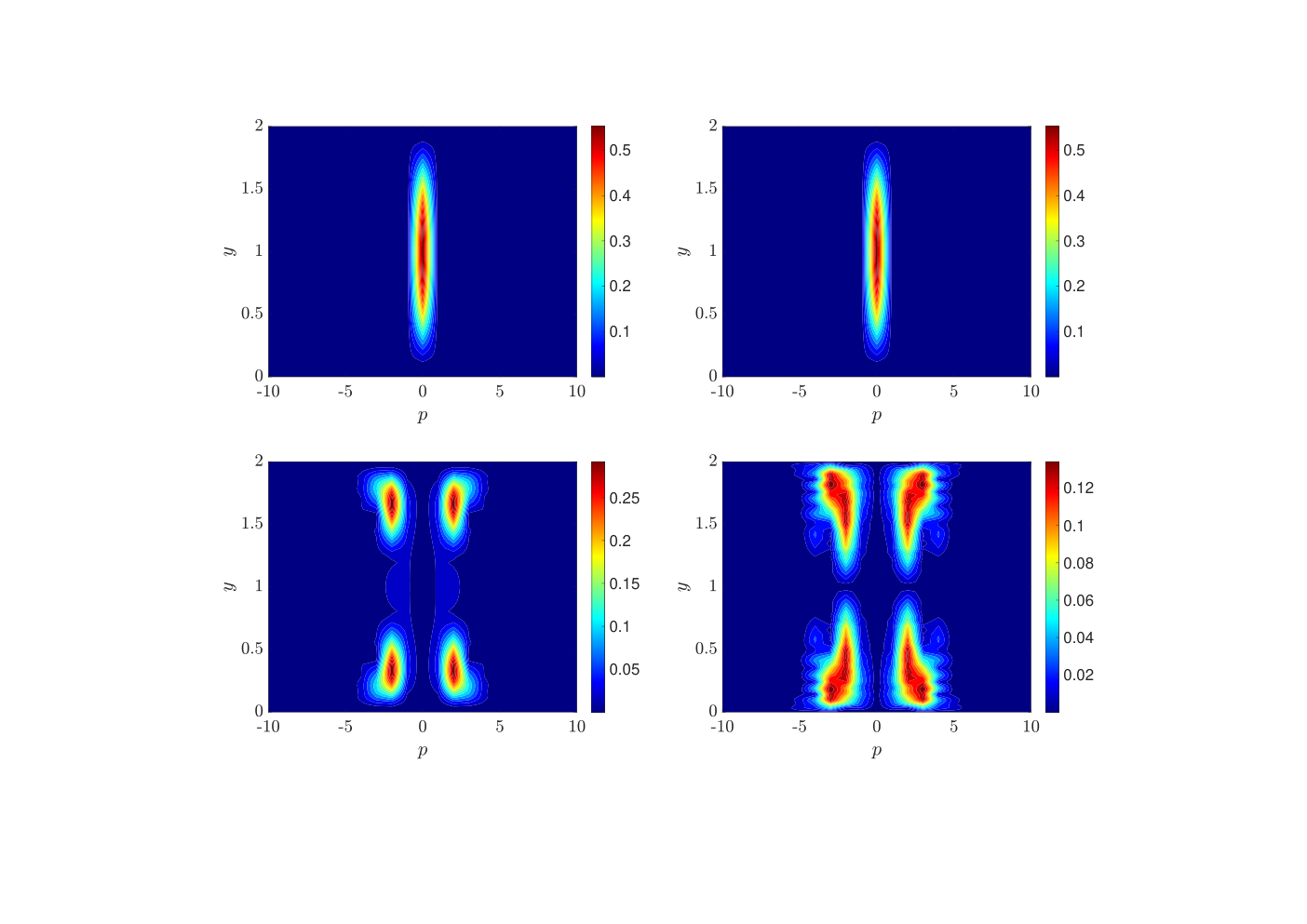
The truncation factor in Eq.(12) defines the spectral expansion of the flow variables in the streamwise direction. The computed values of both and should be robust to the chosen value of — a parameter which also strongly affects the computational cost.
Since in non-modal stability analyses the optimal perturbation is not constrained to a single streamwise wavenumber, should be sufficiently large to guarantee a compact support for the optimal initial condition, while also accurately capturing its evolution up to the time of maximum energy growth. We have empirically established that the optimal initial conditions obtained by varying the problem parameters can be grouped into two broad classes with qualitatively different characteristics in terms of spectral content. Figure 11 shows, for the two classes of optimal initial conditions, how their amplitude depends on the wall-normal coordinate and on the modal expansion index . In the first class (top row of figure 11), the -component is largest at , i.e. , whereas the -component is largest near the walls at . In the second class (bottom row), both and show maxima at a wavenumber inversely proportional to . The temporal evolutions of perturbations from either class are qualitatively similar.
Owing to the procedural complexity of properly selecting the parameter , our operational choice is to enforce a dynamical and automated adjustment of . Each simulation is started with a reasonable first guess , and then is incremented by unitary steps until a most unstable eigenvalue is computed that satisfies the criterion
| (24) |
The initial guess is selected by empirically accounting for the two distributions discussed above, according to the following heuristics that depends on the forcing parameters:
| (25) |
Once is set, an iterative increase of is started until the termination criterion (24) is satisfied (or a maximum value of is reached). Across the entire study, this iteration always terminated before the limit is reached, and the largest value used within our study was .
| 231.1303 | 231.1788 | 231.2086 | 231.2300 | 231.2390 |
Provided that is not too low, the values of are not particularly sensitive to , as shown in table 4. For this case, our procedure leads to , and the relative change of for value of between and is bounded by .
A.3 Number of eigenvalues
The fraction of the entire set of eigenvalues of the system matrix retained in the iterative Arnoldi procedure must ensure that the dynamics of the optimal initial condition is well represented. The number of retained eigenvalues defines the truncation operator T, which reduces the size of the matrix and with it the cost of computing the transient growth rate (22).
The worst-case scenario corresponds to optimal initial conditions of the type illustrated in the bottom row of Figure 11. For one such case (namely , and ), table 5 reports the computed value of as is changed, for selected values of . The sensitivity is certainly non-negligible, especially at the lower . By examining this case as well as other representative cases, we arrive at the operational choice of setting when , and otherwise.
| 0.5 | 20.2629 | 20.7811 | 20.8603 | 20.8655 | 20.8657 | 20.8657 | |
| 0.75 | 15.0971 | 15.1162 | 15.1261 | 15.1266 | 15.1266 | 15.1266 | |
| 1 | 13.1278 | 13.1681 | 13.1957 | 13.2004 | 13.2013 | 13.2015 | |
| 1.5 | 12.4396 | 12.4427 | 12.4431 | 12.4432 | 12.4433 | 12.4437 | |
| 2.5 | 10.0582 | 10.0583 | 10.0584 | 10.0585 | 10.0588 | 10.0590 | |
| 3.5 | 10.4932 | 10.4934 | 10.4937 | 10.4938 | 10.4941 | 10.4943 | |
| 5 | 10.9079 | 10.9081 | 10.9084 | 10.9084 | 10.9087 | 10.9089 |
A.4 Temporal discretization
A temporal integration step must be chosen to evaluate (22) and to identify the maximum and the time at which it occurs. In classic, unforced Poiseuille flow, the transient growth function monotonically increases from a unit value at (as long as is above the critical value for monotonic stability) up to , and then steadily decreases. However, when the flow is modified by the SSL, the ensuing presents two local maxima: one is similar to the unforced maximum, the other is directly linked to the SSL. The latter is centered on a considerably narrow peak of the function, and typically occurs at shorter times. The absolute maximum can pertain to either peak, depending on the specific case.

The location of the two peaks varies significantly with the physical parameters of the problem. Figure 12 shows, for a typical case with dominating first peak ( and ), the temporal position of the peak as a function of and . It is seen that, especially at small , occurs at very short times, whereas for small the time scale of the maximum increases, and the unforced peak is recovered. It is also noticed that the first peak of is always located at . Hence our operational choice is to employ a variable time discretization by setting for and increasing it to for .
References
- (1)
- (2) Quadrio, M. ; Ricco, P. ; Viotti, C.: Streamwise-Traveling Waves of Spanwise Wall Velocity for Turbulent Drag Reduction. In: J. Fluid Mech. 627 (2009), S. 161–178
- (3) Quadrio, M.: Drag Reduction in Turbulent Boundary Layers by In-Plane Wall Motion. In: Phil. Trans. R. Soc. A 369 (2011), Nr. 1940, S. 1428–1442
- (4) Leschziner, M. A.: Friction-Drag Reduction by Transverse Wall Motion – A Review. In: J. Mech. 36 (2020), Nr. 5, S. 649–663. – ISSN 1727–7191, 1811–8216
- (5) Ricco, P. ; Skote, M. ; Leschziner, M. A.: A Review of Turbulent Skin-Friction Drag Reduction by near-Wall Transverse Forcing. In: Prog. Aero. Sci. 123 (2021), S. 100713. – ISSN 0376–0421
- (6) Quadrio, M. ; Ricco, P.: Critical Assessment of Turbulent Drag Reduction through Spanwise Wall Oscillation. In: J. Fluid Mech. 521 (2004), S. 251–271
- (7) Banchetti, J. ; Luchini, P. ; Quadrio, M.: Turbulent Drag Reduction over Curved Walls. In: J. Fluid Mech. 896 (2020), S. 1–23
- (8) Quadrio, M. ; Chiarini, A. ; Banchetti, J. ; Gatti, D. ; Memmolo, A. ; Pirozzoli, S.: Drag Reduction on a Transonic Airfoil. In: J. Fluid. Mech. 942 (2022), S. R2, 1–10. – ISSN 0022–1120, 1469–7645
- (9) Yakeno, A.: Drag Reduction and Transient Growth of a Streak in a Spanwise Wall-Oscillatory Turbulent Channel Flow. In: Phys. Fluids 33 (2021), Nr. 6, S. 065122. – ISSN 1070–6631
- (10) Auteri, F. ; Baron, A. ; Belan, M. ; Campanardi, G. ; Quadrio, M.: Experimental Assessment of Drag Reduction by Traveling Waves in a Turbulent Pipe Flow. In: Phys. Fluids 22 (2010), Nr. 11, S. 115103/14
- (11) Marusic, I. ; Chandran, D. ; Rouhi, A. ; Fu, M.K. ; Wine, D. ; Holloway, B. ; Chung, D. ; Smits, A.J.: An Energy-Efficient Pathway to Turbulent Drag Reduction. In: Nat Commun 12 (2021), Nr. 1, S. 5805. – ISSN 2041–1723
- (12) Gouder, K. ; Potter, M. ; Morrison, J.F.: Turbulent Friction Drag Reduction Using Electroactive Polymer and Electromagnetically Driven Surfaces. In: Exp. Fluids 54 (2013), Nr. 1, S. 1441
- (13) Gatti, D. ; Güttler, A. ; Frohnapfel, B. ; Tropea, C.: Experimental Assessment of Spanwise-Oscillating Dielectric Electroactive Surfaces for Turbulent Drag Reduction in an Air Channel Flow. In: Exp. Fluids 56 (2015), Nr. 5, S. 1–15
- (14) Bird, J. ; Santer, M. ; Morrison, J.F.: Experimental Control of Turbulent Boundary Layers with In-plane Travelling Waves. In: Flow Turbulence Combust 100 (2018), Nr. 4, S. 1015–1035. – ISSN 1573–1987
- (15) Jovanović, M.R.: Turbulence Suppression in Channel Flows by Small Amplitude Transverse Wall Oscillations. In: Physics of Fluids 20 (2008), Nr. 1, S. 014101. – ISSN 1070–6631
- (16) Ricco, P.: Laminar Streaks with Spanwise Wall Forcing. In: Phys. Fluids 23 (2011), Nr. 064103
- (17) Rabin, S.M.E. ; Caulfield, C.P. ; Kerswell, R.R.: Designing a More Nonlinearly Stable Laminar Flow via Boundary Manipulation. In: J. Fluid Mech. 738 (2014), Nr. R1, S. 1–12
- (18) Hack, M. J. P. ; Zaki, T. A.: The Continuous Spectrum of Time-Harmonic Shear Layers. In: Phys. Fluids 24 (2012), Nr. 3, S. 034101
- (19) Hack, M.J.P. ; Zaki, T.A.: The Influence of Harmonic Wall Motion on Transitional Boundary Layers. In: J. Fluid Mech. 760 (2014), S. 63–94
- (20) Hack, M.J.P. ; Zaki, T.A.: Modal and Non-Modal Stability of Boundary Layers Forced by Spanwise Wall Oscillations. In: J. Fluid Mech. 778 (2015), S. 389–427
- (21) Wang, Y. ; Liu, C.: Liutex (Vortex) Cores in Transitional Boundary Layer with Spanwise-Wall Oscillation. In: J Hydrodyn. 31 (2019), Nr. 6, S. 1178–1189
- (22) Duque-Daza, C.A. ; Baig, M.F. ; Lockerby, D.A. ; Chernyshenko, S.I. ; Davies, C.: Modelling Turbulent Skin-Friction Control Using Linearised Navier-Stokes Equations. In: J. Fluid Mech. 702 (2012), S. 403–414
- (23) Negi, P. S. ; Mishra, M. ; Skote, M.: DNS of a Single Low-Speed Streak Subject to Spanwise Wall Oscillations. In: Flow Turbulence Combust 94 (2015), Juni, Nr. 4, S. 795–816. – ISSN 1573–1987
- (24) Negi, P. S. ; Mishra, M. ; Schlatter, P. ; Skote, M.: Bypass Transition Delay Using Oscillations of Spanwise Wall Velocity. In: Phys. Rev. Fluids 4 (2019), Juni, Nr. 6, S. 063904
- (25) Viotti, C. ; Quadrio, M. ; Luchini, P.: Streamwise Oscillation of Spanwise Velocity at the Wall of a Channel for Turbulent Drag Reduction. In: Phys. Fluids 21 (2009), S. 115109
- (26) Floryan, J.M.: Stability of Wall-Bounded Shear Layers in the Presence of Simulated Distributed Roughness. In: J. Fluid Mech. 335 (1997), S. 29–55
- (27) Szumbarski, J. ; Floryan, J. M.: Transient Disturbance Growth in a Corrugated Channel. In: J. Fluid Mech. 568 (2006), Dezember, S. 243–272. – ISSN 1469–7645, 0022–1120
- (28) Schmid, P.J. ; Henningson, D.S.: Stability and Transition in Shear Flows. Springer, 2001
- (29) Quadrio, M. ; Ricco, P.: The Laminar Generalized Stokes Layer and Turbulent Drag Reduction. In: J. Fluid Mech. 667 (2011), S. 135–157
- (30) Abramowitz, M. ; Stegun, I.A.: Handbook of Mathematical Functions. National Bureau of Standards, 1964 (Applied Mathematics Series 55)
- (31) Boyd, J.P.: Chebyshev and Fourier Spectral Methods. 1st. Springer-Verlag, 1989
- (32) Canuto, C. ; Hussaini, M. Y. ; Quarteroni, A. ; Zang, T. A.: Spectral Methods - Fundamentals in Single Domains. Springer, 2006
- (33) Canuto, C. ; Hussaini, M. Y. ; Quarteroni, A. ; Zang, T. A.: Spectral Methods. Evolution to Complex Geometries and Applications to Fluid Dynamics. Springer, 2007
- (34) Trefethen, L.N. ; Bau, D. I.: Numerical Linear Algebra. Siam, 1997
- (35) Reddy, S.C. ; Henningson, D.S.: Energy Growth in Viscous Channel Flows. In: J. Fluid Mech. 252 (1993), S. 209–238
- (36) Criminale, W.O. ; Jackson, T.L.: Theory and Computation of Hydrodynamic Stability. Cambridge University Press, 2003
- (37) Clenshaw, C.W. ; Curtis, A.R.: A Method for Numerical Integration on an Automatic Computer. In: Numer. Math. 2 (1960), Nr. 1, S. 197–205
- (38) Imhof, J.P.: On the Method for Numerical Integration of Clenshaw and Curtis. In: Numer. Math. 5 (1963), Nr. 1, S. 138–141
- (39) Hanifi, A. ; Schmid, P. ; Henningson, D.: Transient Growth in Compressible Boundary Layer Flow. In: Phys. Fluids (1996)
- (40) Maleknejad, K. ; Lotfi, T.: Numerical Expansion Methods for Solving Integral Equations by Interpolation and Gauss Quadrature Rules. In: Appl. Math. Comput. 168 (2005), Nr. 1, S. 111–124
- (41) Luchini, P. ; Quadrio, M.: A Low-Cost Parallel Implementation of Direct Numerical Simulation of Wall Turbulence. In: J. Comp. Phys. 211 (2006), Nr. 2, S. 551–571
- (42) Orr, W. M. F.: The Stability or Instability of the Steady Motions of a Perfect Liquid and of a Viscous Liquid. Part II. A Viscous Liquid. In: Proc R Ir. Acad Sect Math Phys Sci 27 (1907), S. 69–138
- (43) Schmid, P.: Nonmodal Stability Theory. In: Annu. Rev. Fluid Mech. 39 (2007), S. 129–162
- (44) Skote, M. ; Mishra, M. ; Wu, Y.: Wall Oscillation Induced Drag Reduction Zone in a Turbulent Boundary Layer. In: Flow Turbulence Combust 102 (2019), Nr. 3, S. 641–666. – ISSN 1573–1987
- (45) Martinelli, F. ; Quadrio, M. ; Schmid, P.J.: Linear Stability of Poiseuille Flow over the Generalized Stokes Layer. In: Euromech Turbulence Conference XIII, Warsaw (PL), Sept. 12-15, 2011, 2011
- (46) Orszag, S. A.: Accurate Solution of the Orr-Sommerfeld Stability Equation. In: J. Fluid Mech. 50 (1971), Nr. 4, S. 689–703
- (47) Reddy, S.C. ; Schmid, P.J. ; Henningson, D.S.: Pseudospectra of the Orr-Sommerfeld Operator. In: SIAM J. Appl. Math. 53 (1993), Nr. 1, S. 15–47
- (48) Harfash, A.J.: Numerical Methods for Solving Some Hydrodynamic Stability Problems. In: Int. J. Appl. Comput. Math. 1 (2015), Nr. 2, S. 293–326