ShadowNet for Data-Centric Quantum System Learning
Abstract
Understanding the dynamics of large quantum systems is hindered by the curse of dimensionality. Statistical learning offers new possibilities in this regime by neural-network protocols and classical shadows, while both methods have limitations: the former is plagued by the predictive uncertainty and the latter lacks the generalization ability. Here we propose a data-centric learning paradigm combining the strength of these two approaches to facilitate diverse quantum system learning (QSL) tasks. Particularly, our paradigm utilizes classical shadows along with other easily obtainable information of quantum systems to create the training dataset, which is then learnt by neural networks to unveil the underlying mapping rule of the explored QSL problem. Capitalizing on the generalization power of neural networks, this paradigm can be trained offline and excel at predicting previously unseen systems at the inference stage, even with few state copies. Besides, it inherits the characteristic of classical shadows, enabling memory-efficient storage and faithful prediction. These features underscore the immense potential of the proposed data-centric approach in discovering novel and large-scale quantum systems. For concreteness, we present the instantiation of our paradigm in quantum state tomography and direct fidelity estimation tasks and conduct numerical analysis up to 60 qubits. Our work showcases the profound prospects of data-centric artificial intelligence to advance QSL in a faithful and generalizable manner.
I Introduction
The precise characterization of quantum systems holds paramount significance in the development, validation, and evaluation of emerging quantum technologies eisert2020quantum; gebhart2023learning. However, the rapid progress of quantum technologies presents an escalating challenge in fully describing modern quantum devices, since a general -qubit state tomography necessitates exponential state replicas with for a reliable estimation gross2010quantum; blume2010optimal; flammia2012quantum; sugiyama2013precision; haah2016sample; o2016efficient; kueng2017low. Fortunately, many physical scenarios offer a ray of hope as the structural information about the target systems is known, allowing scenario-specific models to learn large-scale quantum systems efficiently. As a result, great efforts have been made to designing effective models for quantum system learning (QSL), encompassing tasks such as low-entangled state reconstruction cramer2010efficient; landon2012practical; lanyon2017efficient, randomized benchmarking knill2008randomized; magesan2012efficient; helsen2022general, direct fidelity estimation flammia2011direct; huang2020predicting; elben2022randomized, Hamiltonian learning granade2012robust; bairey2019learning; huang2023learning, and self-testing mayers2003self; montanaro2013survey; vsupic2020self. Although diverse in specific tasks, all models share a common target: fast acquire the interested information of the quantum system and minimize the number of required state copies.
Statistical learning algorithms are leading candidates to tackle QSL tasks, due to their intrinsic data-driven nature aaronson2007learnability; mohri2018foundations. Two prominent solutions in this context are shadow tomography aaronson2018shadow and neural-network-based QSL (NN-QSL) torlai2018neural; gao2018experimental; zhu2022flexible; wang2022predicting. Shadow tomography stands on the fact that many practical QSL tasks only require accurate predictions of specific properties of quantum systems, rather than their full classical descriptions. Myriad algorithms have been proposed to complete shadow tomography aaronson2018online; chen2022adaptive; lumbreras2022multi. Among them, the most viable one is classical shadows huang2020predicting, requiring only polynomial state copies to predict an exponential number of target functions. In parallel, NN-QSL makes use of the strong power of deep neural networks (DNNs) to learn a class of quantum states with similar structures by extracting their hidden features 11 1 The literature related to NN-QSL can be divided into two categories. This first class is using DNN to learn a specific state, which treats QSL as an optimization task and the optimized DNN cannot be used to other states. The second class is using DNN to learn a class of states, where the learnt information can be used to predict new states from the same class. See SM A for explanations.. Over the past years, varied architectures of DNNs have been proposed to tackle different QSL tasks, capitalizing on the enhanced efficiency carrasquilla2019reconstructing; torlai2019integrating; xin2019local; ahmed2021quantum; quek2021adaptive; morawetz2021u; cha2021attention; lange2022adaptive; koutny2022neural; schmale2022efficient; zhang2022efficient; an2023unified and generalization ability wu2023quantum; zhang2021direct; smith2021efficient; zhong2022quantum; lohani2023dimension.

Despite their promising potential, both classical shadows and NN-QSL exhibit manifest limitations. Classical shadows and its variants lack generalizability, hinting the inability of extracting the knowledge from a class of states to reduce the sample complexity towards the desired estimation accuracy. On the other hand, although some NN-QSL protocols address this issue assisted by the supervised learning framework, concerns arise regarding the faithfulness of its output at the inference stage gao2018experimental; zhu2022flexible. This deficiency poses a critical challenge of using NN-QSL to learn unseen quantum systems, as the predictions may deviate significantly from the ground truth.
In this study, we present a novel learning paradigm, dubbed ShadowNet, which combines the strength of classical shadows and NN-QSL to efficiently, faithfully, and generalizably solve various QSL tasks. A fundamental aspect of ShadowNet lies in establishing a generic construction rule for the dataset used to train NN-QSL, incorporating classical shadows with readily accessible information about the explored quantum system. The emphasis on the importance of the dataset aligns with the concept of data-centric AI, highlighting the crucial role of improving datasets to enhance performance in practical machine learning applications liang2022advances; mazumder2022dataperf. As depicted in Fig. 1(a), training on this dataset provides two attractive benefits: empowered by the generalization ability of DNNs, ShadowNet enables the offline training and fast predicting at the inference stage, even when limited state copies are available; the predictive faithfulness can be evaluated by the estimated properties of classical shadows. These distinctive features hint great potentials of ShadowNet in dealing with unseen quantum systems, and pave the way for using classical shadows as foundational elements in the development of data-centric QSL.
Although the core of QSL dataset is classical shadows and the system information, the detailed formalism of training data is contingent upon the specific problem being addressed, and the learning strategy employed by ShadowNet should be meticulously tailored to accommodate such specific data features. To exhibit the effectiveness of ShadowNet, we instantiate it to solve quantum state tomography and direct fidelity estimation tasks. Notably, the proposed formalism and learning strategy can be extended to tackle other substantial QSL tasks, which may be of independent interest. Numerical results exhibit the efficacy of ShadowNet in acquiring the desired information about the system using a reduced number of copies at the scale of up to 60 qubits.
II Data-centric quantum system learning and ShadowNet
The paradigm of data-centric quantum system learning (QSL) underscores the paramount significance of elevating datasets as a potential avenue to enhance both the efficiency and fidelity of learning models when tackling QSL tasks. This concept stands in contrast to the traditional model-centric QSL approach, which revolves around the utilization of diverse deep learning models for QSL. Precisely, in the realm of data-centric QSL, the construction of datasets should adhere to three fundamental requirements: datasets designed for QSL should be memory efficient; the dimension of data features cannot be the sole computational bottleneck for learning models; data features should contain ample information to facilitate predictive uncertainty estimation while enabling an efficient collection process. Guided by these guiding principles, ShadowNet creates the training dataset as follows. Let be the training dataset, containing examples sampled from the underlying distribution . For the -th example, includes the classical shadows of the target state with snapshots whose magnitude depends on the desired faith (see SM C for explanations), and other possible information that is easily obtained to describe the quantum system. The label depends on the QSL task at hand, e.g., it refers to in state tomography.
Once is prepared, ShadowNet employs a tailored DNN to learn the mapping rule from to (see Fig. 1). Denote as the prediction of DNN with being weights to be optimized. The objective function of ShadowNet is
| (1) |
where the per-sample loss quantifies the prediction error. Throughout the whole study, is specified to the mean-squared loss. The optimization of is completed by the gradient descent methods with in total epochs. The detailed formalism of and implementation of are problem-dependent and will be elucidated later.
During the inference procedure, the optimized ShadowNet can efficiently predict unseen examples , i.e., . A major difference between ShadowNet and prior supervised NN-QSL methods is enabling a faithful prediction of . The predictive faith is computed by its classical shadows, as shown in Fig. 1(c). That is, the prediction returned by ShadowNet should locate into the error bounds of its shadow estimation. Otherwise, the prediction is deemed to be unfaithful and the classical shadows’ estimation is preferred.

ShadowNet advances classical shadows by harnessing DNN’s capability of distilling knowledge from the training dataset. This acquired knowledge enables ShadowNet to achieve a lower estimation error compared to classical shadows, even when utilizing fewer state copies. The synergy of generalization ability, memory efficiency, and faithfulness positions ShadowNet as a powerful solution for learning novel and large-scale quantum systems.
As aforementioned, the formalism of training data and the design of DNN are flexible and dominate the performance of ShadowNet. To provide a concrete illustration, we next introduce the implementation details of ShadowNet for two substantial QSL tasks: quantum state tomography (QST) and direct fidelity estimation (DFE). Note that the proposed methods can be extended to solve other QSL tasks, especially those that can be addressed by classical shadows elben2022randomized.
III ShadowNet for quantum state tomography
QST is the process by which the density matrix of a quantum state is reconstructed using measurements on a set of identical state copies. Conventional QST methods typically optimize each state independently, disregarding the potential relationships among states that may exhibit similar structures and sample from the same underlying distribution . In contrast, ShadowNet handles QST by reframing it as a learning problem rather than an optimization problem. Its primary objective is to extract valuable knowledge of by learning the mapping rule from finite measurement data to the precise density matrix, and then exploits this knowledge to reduce the sample complexity . In this way, ShadowNet possesses the capability of efficiently predicting the density matrix of previously unseen states sampled from , using very few measurements.
When solving -qubit QST, the learning process of ShadowNet resembles the image-denoising task in computer vision buades2005review. Intuitively, the measured data of each state form a ‘noisy image’, and DNN is optimized to acquire a mapping rule for denoising, thereby recovering the ‘precise image’ (i.e., the density matrix). More formally, the learning procedure involves utilizing the reconstructed shadow state as input and the corresponding exact density matrix as the label . Denote as classical shadows of collected by random Pauli-based measurements, where is a Pauli operator and , . The explicit form of the data feature in Eq. (1) is defined as
| (2) |
In the training process, the reconstructed shadow state is fed into DNN and the denoised state is denoted by . To ensure that is physical, ShadowNet adopts a handcrafted DNN to learn the mapping rule from to , formed by the attention mechanism vaswani2017attention and a density-matrix constraint layer ahmed2021quantum. The per-sample loss in Eq. (1) yields , quantifying the reconstruction error with the Frobenius norm. Note that besides attention mechanism, convolutional mechanism and other advanced protocols can also realize ShadowNet. Refer to SM D for the elaboration.
At the inference stage, ShadowNet exhibits an advantage by directly predicting the density matrix of previously unseen states, using only the reconstructed shadow state as input, without requiring additional optimization. This feature pinpoints the superior efficiency of ShadowNet in comparison to optimization-based QST methods, which often entail lengthy post-processing procedures monz201114. Besides, unlike prior NN-QST, ShadowNet allows the faithful prediction. Note that although fidelity is a standard metric for assessing the faithfulness in QST, exponential state copies are essential to ensure a reliable estimation. In this regard, a surrogate quantity may be adopted to gauge the faithfulness, which leverages prior information about the explored quantum system. For example, when learning a class of ground states, corresponds to the ground energies. The reconstructed state is judged to be faithful if the estimated ground state energy falls into the error bounds of its shadow estimation .
We test ShadowNet on reconstructing ground states of two quantum spin systems: one-dimensional transverse-field Ising model (TFIM) and XXZ model. Both systems are crucial for many-body quantum simulations and have been widely explored torlai2018neural; zhu2022flexible; carrasquilla2019reconstructing; schmale2022efficient. The explicit expression of TFIM is , where denotes the neighborhood spins, and and stand for interaction strength and the transverse field, respectively. The explicit form of XXZ model is , where refers to the coupling parameter. In the simulations, the number of qubits is set as for both Hamiltonians. The performance of ShadowNet is evaluated by two metrics: the fidelity ; the estimation error of the ground energy .
The simulation results are illustrated in Fig. 2. In the first task, we apply ShadowNet to learn the ground states of TFIM. To collect the training and test datasets, we fix and sample uniformly from the interval to obtain different examples. The number of measurements for classical shadows is . When the size of training dataset is , the simulation results are exhibited in Fig. 2(a). The left panel indicates that after training epochs, the training fidelity is near to and the estimation error of the ground energy is around zero. Moreover, ShadowNet has a satisfied generalizable ability after epochs. The test fidelity on unseen ground states are near to . Meanwhile, the ground energy estimation error is almost zero, which is . The right panel showcases the predictive faith of ShadowNet on five test instances in terms of . The results reflect that the predictions of ShadowNet fall into the error bound of classical shadows and are closer to the exact results.
We then explore how the dataset size affects the performance of ShadowNet. All hyper-parameter settings are kept to be the same with the above experiment, except for the varied dataset size, i.e., . The simulation results are visualized in Fig. 2(b). When decreasing from to , the test fidelity drops from to and the test estimation error increases from to . These results suggest that a modest size of dataset is necessary to warrant the performance of ShadowNet.
The last task related to TFIM is investigating the role of the shot number . All hyper-parameter settings are the same with the previous experiments, except for two modifications. First, the shot number has three varied settings, i.e., . Second, when constructing training and test datasets, the range of the interaction strength expands to , leading to the increased diversity of examples. The simulation results of ShadowNet are shown in Fig. 2(c). An immediate observation is that when exceeds a threshold, the performance of ShadowNet tends to be optimal. In other words, the shot number should be carefully selected in ShadowNet, since continuously increasing does not only require expensively computational cost, but also narrows the advance of ShadowNet compared to classical shadows.
We next apply ShadowNet to tackle a more difficult QST task, where the ground states are collected from TFIM and XXZ model. For both the training and test datasets, the construction rule related to TFIM is identical to the third task introduced above. For XXZ model, we set for and uniformly sample from to generate training and test examples. The training dataset contains the equivalent number of ground states from TFIM and XXZ model. We fix and , and vary the settings of and to evaluate the performance of ShadowNet.
| Performance | ||||||||
|---|---|---|---|---|---|---|---|---|
|
|
|||||||
| 500 | 100 | 0.477 0.204 | ||||||
| 800 | ||||||||
| 1000 | 100 | 0.308 0.102 | ||||||
| 800 | ||||||||
| 2000 | 100 | 0.204 0.039 | ||||||
| 800 | ||||||||
The achieved results are summarized in Table 1. Particularly, when and , the test fidelity is almost optimal and the estimation error is near to zero. These observations accord with the results of TFIM, i.e., the size of training dataset dominates the performance of ShadowNet when excesses a threshold. In addition, ShadowNet dramatically outperforms classical shadows with sufficient training data, i.e., versus when and . This result suggests the superiority of ShadowNet in learning complex quantum systems since it can attain the desired estimation using significantly fewer samples compared to classical shadows. Refer to SM E for more analysis, including the omitted simulation details and the evaluation of ShadowNet under the convolutional mechanisms.
IV ShadowNet for direct fidelity estimation
DFE is a crucial measure in assessing the quality of quantum states prepared by quantum machines flammia2011direct. Mathematically, DFE measures the similarity between the desired pure state and the actual state , i.e., . In the quest to certify large-scale quantum devices, the primary objective of DFE algorithms is to obtain accurate estimations of with few measurements and efficient post-processing kliesch2021theory. Similarly to QST, conventional approaches focus on individual states, neglecting the inherent relationships among a class of states and consequently facing challenges in terms of either sample complexity or post-processing runtime cost. Despite initial attempts to tackle these challenges by leveraging DNNs, the existing methods lack a guarantee of predictive faithfulness zhang2021direct; zhu2022flexible.
ShadowNet addresses the above issues by harnessing the complementary roles of classical shadows and DNNs. To cope with the large-qubit scenario, the dataset construction rule devised for DFE deviates from that utilized in QST. Specifically, for an -qubit DFE task, the data feature of the -th example in the dataset yields
| (3) |
where is the vectorization operation, refers to the local inverse snapshot at the -th qubit, and includes the information of the quantum device (e.g., the global depolarization error rate). Let in Eq. (2) be the classical shadows of the prepared state with random Pauli-based measurements. The local inverse snapshot is defined as . The corresponding label represents the accurate fidelity, i.e., . Such a construction rule embraces two compelling benefits: (i) it enables the scalability of ShadowNet in handling large-scale qubit systems, since the dimension of linearly scales with the qubit count ; (ii) the incorporation of accessible information into allows DNN to effectively capture the mapping rule connecting the measured data to precise fidelity values. We remark that the proposed construction rule can be used to diverse QSL tasks, such as entanglement estimation and self-testing.

Once the dataset is prepared according to Eq. (3), ShadowNet exploits the attention mechanism to construct a handcrafted DNN to proceed training. The per-sample loss measures the estimation error of fidelity, i.e., , where is the prediction of the -th example . At the inference stage, the collected classical shadows can be used to quantify the predictive faithfulness, as with QST tasks. Refer to SM D for the omitted details.
We examine the power of ShadowNet in solving DFE on two classes of noisy GHZ states simultaneously. As pictured in Fig. 3(a), the first class is the noisy global GHZ states, i.e., , where is the local depolarization channel applied to the GHZ state , and describes the depolarization error rate of the single-qubit and two-qubit gates, respectively. The second class is the noisy local GHZ states, i.e., , where is the local depolarization channel defined above and . The label of each example amounts to the fidelity between the noisy and ideal states, i.e., or . When collecting training and test examples, we uniformly sample and and fix the shot number for classical shadows to be . The learning performance and predictive faith are measured by . Each setting is repeated with five times to obtain the statistical results.
The simulation results are exhibited in Fig. 3. Our first task is comparing the accuracy of the fidelity estimation between classical shadows (i.e., ) and ShadowNet when and . The subplot (b) illustrates the predictive fidelity on test examples of noisy global GHZ states. ShadowNet can accurately predict the true fidelity, while classical shadows fail to compute the true fidelity when is small. To uncover the advance of ShadowNet, we further adopt the t-distributed stochastic neighbor embedding (t-SNE) algorithm to visualize its learning dynamics during the training van2008visualizing. Fig. 3(c) plots the representations at the last-second layer of ShadowNet when projecting to a two-dimensional plane. Before training, noisy global and local GHZ states locate into two clusters. Meanwhile, the representations of noisy global GHZ states are mixed, implying that ShadowNet cannot accurately predict the fidelity of each state. After training, the representations of noisy global and local GHZ states are well-aligned, enabling the accurate predictions (see SM E for elaborations). We next systematically comprehend how the number of qubits and the size of training dataset affect the prediction accuracy of ShadowNet. To do so, we vary the number of qubits as and the dataset size as . The simulation results are demonstrated in Fig. 3(d). When exceeds a threshold (e.g., ), ShadowNet attains a satisfied performance for all settings of . This phenomenon suggests that the proposed dataset construction rule has the potential to dramatically reduce the required number of training examples, as a crucial characteristic to apply ShadowNet to solve large-scale DFE tasks. Refer to SM E for more numerical results.
V Discussion and outlook
We present the concept of data-centric QSL, emphasizing the central role played by datasets in contrast to the model-centric approaches prevalent in previous NN-QSL methods, which primarily focus on the design of DNN architectures. In this respect, we devise ShadowNet as a flexible and robust paradigm to tackle QSL tasks, with a specific emphasis on the synergy of generalizability, efficiency, and faithfulness. Central to ShadowNet is the utilization of classical shadows, known for their memory efficiency and estimation guarantees, and easily obtained information to create datasets. Due to the flexibility of ShadowNet, we devise two distinct approaches for the dataset construction and model implementation, tailored to the specific requirements of the task at hand. Numerical simulations confirm the efficacy of ShadowNet and exhibit its potential to advance data-centric QSL.
Our work stimulates several important avenues for future research. While our focus has been on Pauli-based random measurements due to their hardware-friendly feature, exploring advanced variants of classical shadows presents an intriguing opportunity to enhance the performance of ShadowNet huang2022learning; nguyen2022optimizing; bertoni2022shallow; hadfield2022measurements; struchalin2021experimental; wei2023neural. Moreover, instead of the discrete quantum systems, the applicability of ShadowNet can be extended to facilitate the learning of continuous-variable quantum systems by leveraging continuous-variable classical shadows to construct the similar training datasets becker2022classical.
Exploring alternative construction rules and expanding the applications of ShadowNet represent a critical avenue for further research. In the context of DFE, we leverage the noise information inherent in quantum systems to be a part of data feature. As the majority of QSL problems arise from noisy intermediate-scale quantum devices preskill2018quantum, it is intriguing to investigate whether other easily accessible information pertaining to quantum devices can be utilized to construct datasets that aid DNN in extracting underlying mapping rules, even with limited data sizes. For instance, considering the prominence of variational quantum algorithms cerezo2021variational; bharti2021noisy; tian2023recent; li2022recent; du2022quantum as a major application for near-term quantum devices, the design of novel data-centric QSL models to enhance the characterization and error mitigation of the output of these algorithms bennewitz2022neural; jnane2023quantum emerges as a desirable direction.
References
- (1) Jens Eisert, Dominik Hangleiter, Nathan Walk, Ingo Roth, Damian Markham, Rhea Parekh, Ulysse Chabaud, and Elham Kashefi. Quantum certification and benchmarking. Nature Reviews Physics, 2(7):382–390, 2020.
- (2) Valentin Gebhart, Raffaele Santagati, Antonio Andrea Gentile, Erik M Gauger, David Craig, Natalia Ares, Leonardo Banchi, Florian Marquardt, Luca Pezzè, and Cristian Bonato. Learning quantum systems. Nature Reviews Physics, 5(3):141–156, 2023.
- (3) David Gross, Yi-Kai Liu, Steven T Flammia, Stephen Becker, and Jens Eisert. Quantum state tomography via compressed sensing. Physical review letters, 105(15):150401, 2010.
- (4) Robin Blume-Kohout. Optimal, reliable estimation of quantum states. New Journal of Physics, 12(4):043034, 2010.
- (5) Steven T Flammia, David Gross, Yi-Kai Liu, and Jens Eisert. Quantum tomography via compressed sensing: error bounds, sample complexity and efficient estimators. New Journal of Physics, 14(9):095022, 2012.
- (6) Takanori Sugiyama, Peter S Turner, and Mio Murao. Precision-guaranteed quantum tomography. Physical Review Letters, 111(16):160406, 2013.
- (7) Jeongwan Haah, Aram W Harrow, Zhengfeng Ji, Xiaodi Wu, and Nengkun Yu. Sample-optimal tomography of quantum states. In Proceedings of the forty-eighth annual ACM symposium on Theory of Computing, pages 913–925, 2016.
- (8) Ryan O’Donnell and John Wright. Efficient quantum tomography. In Proceedings of the forty-eighth annual ACM symposium on Theory of Computing, pages 899–912, 2016.
- (9) Richard Kueng, Holger Rauhut, and Ulrich Terstiege. Low rank matrix recovery from rank one measurements. Applied and Computational Harmonic Analysis, 42(1):88–116, 2017.
- (10) Marcus Cramer, Martin B Plenio, Steven T Flammia, Rolando Somma, David Gross, Stephen D Bartlett, Olivier Landon-Cardinal, David Poulin, and Yi-Kai Liu. Efficient quantum state tomography. Nature communications, 1(1):149, 2010.
- (11) Olivier Landon-Cardinal and David Poulin. Practical learning method for multi-scale entangled states. New Journal of Physics, 14(8):085004, 2012.
- (12) BP Lanyon, C Maier, Milan Holzäpfel, Tillmann Baumgratz, C Hempel, P Jurcevic, Ish Dhand, AS Buyskikh, AJ Daley, Marcus Cramer, et al. Efficient tomography of a quantum many-body system. Nature Physics, 13(12):1158–1162, 2017.
- (13) Emanuel Knill, Dietrich Leibfried, Rolf Reichle, Joe Britton, R Brad Blakestad, John D Jost, Chris Langer, Roee Ozeri, Signe Seidelin, and David J Wineland. Randomized benchmarking of quantum gates. Physical Review A, 77(1):012307, 2008.
- (14) Easwar Magesan, Jay M Gambetta, Blake R Johnson, Colm A Ryan, Jerry M Chow, Seth T Merkel, Marcus P Da Silva, George A Keefe, Mary B Rothwell, Thomas A Ohki, et al. Efficient measurement of quantum gate error by interleaved randomized benchmarking. Physical review letters, 109(8):080505, 2012.
- (15) Jonas Helsen, Ingo Roth, Emilio Onorati, Albert H Werner, and Jens Eisert. General framework for randomized benchmarking. PRX Quantum, 3(2):020357, 2022.
- (16) Steven T Flammia and Yi-Kai Liu. Direct fidelity estimation from few pauli measurements. Physical review letters, 106(23):230501, 2011.
- (17) Hsin-Yuan Huang, Richard Kueng, and John Preskill. Predicting many properties of a quantum system from very few measurements. Nature Physics, 16(10):1050–1057, 2020.
- (18) Andreas Elben, Steven T Flammia, Hsin-Yuan Huang, Richard Kueng, John Preskill, Benoît Vermersch, and Peter Zoller. The randomized measurement toolbox. Nature Reviews Physics, pages 1–16, 2022.
- (19) Christopher E Granade, Christopher Ferrie, and Nathan Wiebe. Robust online hamiltonian learning. New Journal of Physics, 14(10):103013, 2012.
- (20) Eyal Bairey, Itai Arad, and Netanel H Lindner. Learning a local hamiltonian from local measurements. Physical review letters, 122(2):020504, 2019.
- (21) Hsin-Yuan Huang, Yu Tong, Di Fang, and Yuan Su. Learning many-body hamiltonians with heisenberg-limited scaling. Physical Review Letters, 130(20):200403, 2023.
- (22) Dominic Mayers and Andrew Yao. Self testing quantum apparatus. arXiv preprint quant-ph/0307205, 2003.
- (23) Ashley Montanaro and Ronald de Wolf. A survey of quantum property testing. arXiv preprint arXiv:1310.2035, 2013.
- (24) Ivan Šupić and Joseph Bowles. Self-testing of quantum systems: a review. Quantum, 4:337, 2020.
- (25) Scott Aaronson. The learnability of quantum states. Proceedings of the Royal Society A: Mathematical, Physical and Engineering Sciences, 463(2088):3089–3114, 2007.
- (26) Mehryar Mohri, Afshin Rostamizadeh, and Ameet Talwalkar. Foundations of machine learning. MIT press, 2018.
- (27) Scott Aaronson. Shadow tomography of quantum states. In Proceedings of the 50th annual ACM SIGACT symposium on theory of computing, pages 325–338, 2018.
- (28) Giacomo Torlai, Guglielmo Mazzola, Juan Carrasquilla, Matthias Troyer, Roger Melko, and Giuseppe Carleo. Neural-network quantum state tomography. Nature Physics, 14(5):447–450, 2018.
- (29) Jun Gao, Lu-Feng Qiao, Zhi-Qiang Jiao, Yue-Chi Ma, Cheng-Qiu Hu, Ruo-Jing Ren, Ai-Lin Yang, Hao Tang, Man-Hong Yung, and Xian-Min Jin. Experimental machine learning of quantum states. Physical review letters, 120(24):240501, 2018.
- (30) Yan Zhu, Ya-Dong Wu, Ge Bai, Dong-Sheng Wang, Yuexuan Wang, and Giulio Chiribella. Flexible learning of quantum states with generative query neural networks. Nature Communications, 13(1):6222, 2022.
- (31) Haoxiang Wang, Maurice Weber, Josh Izaac, and Cedric Yen-Yu Lin. Predicting properties of quantum systems with conditional generative models. arXiv preprint arXiv:2211.16943, 2022.
- (32) Scott Aaronson, Xinyi Chen, Elad Hazan, Satyen Kale, and Ashwin Nayak. Online learning of quantum states. Advances in neural information processing systems, 31, 2018.
- (33) Xinyi Chen, Elad Hazan, Tongyang Li, Zhou Lu, Xinzhao Wang, and Rui Yang. Adaptive online learning of quantum states. arXiv preprint arXiv:2206.00220, 2022.
- (34) Josep Lumbreras, Erkka Haapasalo, and Marco Tomamichel. Multi-armed quantum bandits: Exploration versus exploitation when learning properties of quantum states. Quantum, 6:749, 2022.
- (35) The literature related to NN-QSL can be divided into two categories. This first class is using DNN to learn a specific state, which treats QSL as an optimization task and the optimized DNN cannot be used to other states. The second class is using DNN to learn a class of states, where the learnt information can be used to predict new states from the same class. See SM A for explanations.
- (36) Juan Carrasquilla, Giacomo Torlai, Roger G Melko, and Leandro Aolita. Reconstructing quantum states with generative models. Nature Machine Intelligence, 1(3):155–161, 2019.
- (37) Giacomo Torlai, Brian Timar, Evert PL Van Nieuwenburg, Harry Levine, Ahmed Omran, Alexander Keesling, Hannes Bernien, Markus Greiner, Vladan Vuletić, Mikhail D Lukin, et al. Integrating neural networks with a quantum simulator for state reconstruction. Physical review letters, 123(23):230504, 2019.
- (38) Tao Xin, Sirui Lu, Ningping Cao, Galit Anikeeva, Dawei Lu, Jun Li, Guilu Long, and Bei Zeng. Local-measurement-based quantum state tomography via neural networks. npj Quantum Information, 5(1):109, 2019.
- (39) Shahnawaz Ahmed, Carlos Sánchez Muñoz, Franco Nori, and Anton Frisk Kockum. Quantum state tomography with conditional generative adversarial networks. Physical Review Letters, 127(14):140502, 2021.
- (40) Yihui Quek, Stanislav Fort, and Hui Khoon Ng. Adaptive quantum state tomography with neural networks. npj Quantum Information, 7(1):105, 2021.
- (41) Stewart Morawetz, Isaac JS De Vlugt, Juan Carrasquilla, and Roger G Melko. U (1)-symmetric recurrent neural networks for quantum state reconstruction. Physical Review A, 104(1):012401, 2021.
- (42) Peter Cha, Paul Ginsparg, Felix Wu, Juan Carrasquilla, Peter L McMahon, and Eun-Ah Kim. Attention-based quantum tomography. Machine Learning: Science and Technology, 3(1):01LT01, 2021.
- (43) Hannah Lange, Matjaž Kebrič, Maximilian Buser, Ulrich Schollwöck, Fabian Grusdt, and Annabelle Bohrdt. Adaptive quantum state tomography with active learning. arXiv preprint arXiv:2203.15719, 2022.
- (44) Dominik Koutnỳ, Libor Motka, Zdeněk Hradil, Jaroslav Řeháček, and Luis L Sánchez-Soto. Neural-network quantum state tomography. Physical Review A, 106(1):012409, 2022.
- (45) Tobias Schmale, Moritz Reh, and Martin Gärttner. Efficient quantum state tomography with convolutional neural networks. npj Quantum Information, 8(1):115, 2022.
- (46) Yuan-Hang Zhang and Massimiliano Di Ventra. Efficient quantum state tomography with mode-assisted training. Physical Review A, 106(4):042420, 2022.
- (47) Zheng An, Jiahui Wu, Muchun Yang, DL Zhou, and Bei Zeng. Unified quantum state tomography and hamiltonian learning using transformer models: A language-translation-like approach for quantum systems. arXiv preprint arXiv:2304.12010, 2023.
- (48) Ya-Dong Wu, Yan Zhu, Ge Bai, Yuexuan Wang, and Giulio Chiribella. Quantum similarity testing with convolutional neural networks. Physical Review Letters, 130(21):210601, 2023.
- (49) Xiaoqian Zhang, Maolin Luo, Zhaodi Wen, Qin Feng, Shengshi Pang, Weiqi Luo, and Xiaoqi Zhou. Direct fidelity estimation of quantum states using machine learning. Physical Review Letters, 127(13):130503, 2021.
- (50) Alistair W. R. Smith, Johnnie Gray, and M. S. Kim. Efficient quantum state sample tomography with basis-dependent neural networks. PRX Quantum, 2:020348, Jun 2021.
- (51) Lu Zhong, Chu Guo, and Xiaoting Wang. Quantum state tomography inspired by language modeling. arXiv preprint arXiv:2212.04940, 2022.
- (52) Sanjaya Lohani, Sangita Regmi, Joseph M Lukens, Ryan T Glasser, Thomas A Searles, and Brian T Kirby. Dimension-adaptive machine learning-based quantum state reconstruction. Quantum Machine Intelligence, 5(1):1, 2023.
- (53) Weixin Liang, Girmaw Abebe Tadesse, Daniel Ho, L Fei-Fei, Matei Zaharia, Ce Zhang, and James Zou. Advances, challenges and opportunities in creating data for trustworthy ai. Nature Machine Intelligence, 4(8):669–677, 2022.
- (54) Mark Mazumder, Colby Banbury, Xiaozhe Yao, Bojan Karlaš, William Gaviria Rojas, Sudnya Diamos, Greg Diamos, Lynn He, Douwe Kiela, David Jurado, et al. Dataperf: Benchmarks for data-centric ai development. arXiv preprint arXiv:2207.10062, 2022.
- (55) Antoni Buades, Bartomeu Coll, and Jean-Michel Morel. A review of image denoising algorithms, with a new one. Multiscale modeling & simulation, 4(2):490–530, 2005.
- (56) Ashish Vaswani, Noam Shazeer, Niki Parmar, Jakob Uszkoreit, Llion Jones, Aidan N Gomez, Łukasz Kaiser, and Illia Polosukhin. Attention is all you need. Advances in neural information processing systems, 30, 2017.
- (57) Thomas Monz, Philipp Schindler, Julio T Barreiro, Michael Chwalla, Daniel Nigg, William A Coish, Maximilian Harlander, Wolfgang Hänsel, Markus Hennrich, and Rainer Blatt. 14-qubit entanglement: Creation and coherence. Physical Review Letters, 106(13):130506, 2011.
- (58) Martin Kliesch and Ingo Roth. Theory of quantum system certification. PRX quantum, 2(1):010201, 2021.
- (59) Laurens Van der Maaten and Geoffrey Hinton. Visualizing data using t-sne. Journal of machine learning research, 9(11), 2008.
- (60) Hsin-Yuan Huang. Learning quantum states from their classical shadows. Nature Reviews Physics, 4(2):81–81, 2022.
- (61) H Chau Nguyen, Jan Lennart Bönsel, Jonathan Steinberg, and Otfried Gühne. Optimizing shadow tomography with generalized measurements. Physical Review Letters, 129(22):220502, 2022.
- (62) Christian Bertoni, Jonas Haferkamp, Marcel Hinsche, Marios Ioannou, Jens Eisert, and Hakop Pashayan. Shallow shadows: Expectation estimation using low-depth random clifford circuits. arXiv preprint arXiv:2209.12924, 2022.
- (63) Charles Hadfield, Sergey Bravyi, Rudy Raymond, and Antonio Mezzacapo. Measurements of quantum hamiltonians with locally-biased classical shadows. Communications in Mathematical Physics, 391(3):951–967, 2022.
- (64) GI Struchalin, Ya A Zagorovskii, EV Kovlakov, SS Straupe, and SP Kulik. Experimental estimation of quantum state properties from classical shadows. PRX Quantum, 2(1):010307, 2021.
- (65) Victor Wei, WA Coish, Pooya Ronagh, and Christine A Muschik. Neural-shadow quantum state tomography. arXiv preprint arXiv:2305.01078, 2023.
- (66) Simon Becker, Nilanjana Datta, Ludovico Lami, and Cambyse Rouzé. Classical shadow tomography for continuous variables quantum systems. arXiv preprint arXiv:2211.07578, 2022.
- (67) John Preskill. Quantum computing in the nisq era and beyond. Quantum, 2:79, 2018.
- (68) Marco Cerezo, Andrew Arrasmith, Ryan Babbush, Simon C Benjamin, Suguru Endo, Keisuke Fujii, Jarrod R McClean, Kosuke Mitarai, Xiao Yuan, Lukasz Cincio, et al. Variational quantum algorithms. Nature Reviews Physics, 3(9):625–644, 2021.
- (69) Kishor Bharti, Alba Cervera-Lierta, Thi Ha Kyaw, Tobias Haug, Sumner Alperin-Lea, Abhinav Anand, Matthias Degroote, Hermanni Heimonen, Jakob S Kottmann, Tim Menke, et al. Noisy intermediate-scale quantum algorithms. Reviews of Modern Physics, 94(1):015004, 2022.
- (70) Jinkai Tian, Xiaoyu Sun, Yuxuan Du, Shanshan Zhao, Qing Liu, Kaining Zhang, Wei Yi, Wanrong Huang, Chaoyue Wang, Xingyao Wu, et al. Recent advances for quantum neural networks in generative learning. IEEE Transactions on Pattern Analysis and Machine Intelligence, 2023.
- (71) Weikang Li and Dong-Ling Deng. Recent advances for quantum classifiers. Science China Physics, Mechanics & Astronomy, 65(2):1–23, 2022.
- (72) Yuxuan Du, Tao Huang, Shan You, Min-Hsiu Hsieh, and Dacheng Tao. Quantum circuit architecture search for variational quantum algorithms. npj Quantum Information, 8(1):62, 2022.
- (73) Elizabeth R Bennewitz, Florian Hopfmueller, Bohdan Kulchytskyy, Juan Carrasquilla, and Pooya Ronagh. Neural error mitigation of near-term quantum simulations. Nature Machine Intelligence, 4(7):618–624, 2022.
- (74) Hamza Jnane, Jonathan Steinberg, Zhenyu Cai, H Chau Nguyen, and Bálint Koczor. Quantum error mitigated classical shadows. arXiv preprint arXiv:2305.04956, 2023.
- (75) You Zhou and Qing Liu. Performance analysis of multi-shot shadow estimation. Quantum, 7:1044, 2023.
- (76) Matteo Ippoliti. Classical shadows based on locally-entangled measurements. arXiv preprint arXiv:2305.10723, 2023.
- (77) Hsin-Yuan Huang, Richard Kueng, and John Preskill. Efficient estimation of pauli observables by derandomization. Physical review letters, 127(3):030503, 2021.
- (78) Kouhei Nakaji, Suguru Endo, Yuichiro Matsuzaki, and Hideaki Hakoshima. Measurement optimization of variational quantum simulation by classical shadow and derandomization. Quantum, 7:995, 2023.
- (79) Hsin-Yuan Huang, Michael Broughton, Jordan Cotler, Sitan Chen, Jerry Li, Masoud Mohseni, Hartmut Neven, Ryan Babbush, Richard Kueng, John Preskill, et al. Quantum advantage in learning from experiments. Science, 376(6598):1182–1186, 2022.
- (80) Hsin-Yuan Huang, Richard Kueng, Giacomo Torlai, Victor V Albert, and John Preskill. Provably efficient machine learning for quantum many-body problems. Science, 377(6613):eabk3333, 2022.
- (81) Hong-Ye Hu, Ryan LaRose, Yi-Zhuang You, Eleanor Rieffel, and Zhihui Wang. Logical shadow tomography: Efficient estimation of error-mitigated observables. arXiv preprint arXiv:2203.07263, 2022.
- (82) Alireza Seif, Ze-Pei Cian, Sisi Zhou, Senrui Chen, and Liang Jiang. Shadow distillation: Quantum error mitigation with classical shadows for near-term quantum processors. PRX Quantum, 4(1):010303, 2023.
- (83) Stefan H Sack, Raimel A Medina, Alexios A Michailidis, Richard Kueng, and Maksym Serbyn. Avoiding barren plateaus using classical shadows. PRX Quantum, 3(2):020365, 2022.
- (84) Gregory Boyd and Bálint Koczor. Training variational quantum circuits with covar: covariance root finding with classical shadows. Physical Review X, 12(4):041022, 2022.
- (85) Yuxuan Du, Yibo Yang, Dacheng Tao, and Min-Hsiu Hsieh. Demystify problem-dependent power of quantum neural networks on multi-class classification. arXiv preprint arXiv:2301.01597, 2022.
- (86) Hailan Ma, Zhenhong Sun, Daoyi Dong, Chunlin Chen, and Herschel Rabitz. Attention-based transformer networks for quantum state tomography. arXiv preprint arXiv:2305.05433, 2023.
- (87) Amit Nir, Eran Sela, Roy Beck, and Yohai Bar-Sinai. Machine-learning iterative calculation of entropy for physical systems. Proceedings of the National Academy of Sciences, 117(48):30234–30240, 2020.
- (88) Tailong Xiao, Jingzheng Huang, Hongjing Li, Jianping Fan, and Guihua Zeng. Intelligent certification for quantum simulators via machine learning. npj Quantum Information, 8(1):138, 2022.
- (89) Alexey Dosovitskiy, Lucas Beyer, Alexander Kolesnikov, Dirk Weissenborn, Xiaohua Zhai, Thomas Unterthiner, Mostafa Dehghani, Matthias Minderer, Georg Heigold, Sylvain Gelly, et al. An image is worth 16x16 words: Transformers for image recognition at scale. arXiv preprint arXiv:2010.11929, 2020.
- (90) Jacob Devlin, Ming-Wei Chang, Kenton Lee, and Kristina Toutanova. BERT: pre-training of deep bidirectional transformers for language understanding. In Jill Burstein, Christy Doran, and Thamar Solorio, editors, Proceedings of the 2019 Conference of the North American Chapter of the Association for Computational Linguistics: Human Language Technologies, NAACL-HLT 2019, Minneapolis, MN, USA, June 2-7, 2019, Volume 1 (Long and Short Papers), pages 4171–4186. Association for Computational Linguistics, 2019.
- (91) Jingjing Xu, Xu Sun, Zhiyuan Zhang, Guangxiang Zhao, and Junyang Lin. Understanding and improving layer normalization. Advances in Neural Information Processing Systems, 32, 2019.
- (92) Konrad Banaszek, GM D’ariano, MGA Paris, and MF Sacchi. Maximum-likelihood estimation of the density matrix. Physical Review A, 61(1):010304, 1999.
- (93) Kaiming He, Xiangyu Zhang, Shaoqing Ren, and Jian Sun. Spatial pyramid pooling in deep convolutional networks for visual recognition. IEEE transactions on pattern analysis and machine intelligence, 37(9):1904–1916, 2015.
- (94) Matthew D Zeiler, Dilip Krishnan, Graham W Taylor, and Rob Fergus. Deconvolutional networks. In 2010 IEEE Computer Society Conference on computer vision and pattern recognition, pages 2528–2535. IEEE, 2010.
- (95) Dmitry Ulyanov, Andrea Vedaldi, and Victor Lempitsky. Instance normalization: The missing ingredient for fast stylization. arXiv preprint arXiv:1607.08022, 2016.
- (96) Ville Bergholm, Josh Izaac, Maria Schuld, Christian Gogolin, Shahnawaz Ahmed, Vishnu Ajith, M Sohaib Alam, Guillermo Alonso-Linaje, B AkashNarayanan, Ali Asadi, et al. Pennylane: Automatic differentiation of hybrid quantum-classical computations. arXiv preprint arXiv:1811.04968, 2018.
- (97) Giacomo Torlai and Matthew Fishman. PastaQ: A package for simulation, tomography and analysis of quantum computers, 2020.
SM A Related work
Prior literature related to our work can be classified into three categories, which are classical shadows, neural-network-based quantum state tomography (NN-QST), and other neural-network-based quantum system learning (NN-QSL) protocols. In what follows, we elucidate the connections and distinctions between our work and previous studies falling within each of these categories.
Classical shadows. The primary objective of classical shadows is to efficiently estimate the expectation values of relevant observables using only a limited number of measurements huang2020predicting. Since the inception of classical shadows, researchers have been actively investigating advanced measurement protocols nguyen2022optimizing; zhou2023performance; ippoliti2023classical and de-randomization methods huang2021efficient; nakaji2023measurement that can be efficiently implemented on modern quantum platforms while reducing the number of required measurements for accurate estimation. Additionally, extensive research has been conducted on the various applications of classical shadows, such as solving quantum many-body problems huang2022quantum; huang2022provably, quantum error mitigation hu2022logical; jnane2023quantum; seif2023shadow, and improving variational quantum algorithms sack2022avoiding; boyd2022training; du2022demystify.
Our work complements the existing literature in this domain. Specifically, methods that enhance the capabilities of classical shadows can benefit ShadowNet. Furthermore, as mentioned in the main text, ShadowNet can be extended to tackle QSL tasks that are amenable to classical shadows’ approaches. This complementary role arises from our focus on exploring the memory efficiency and theoretical guarantees of classical shadows in forming the training dataset, which is subsequently learned by deep neural networks to distill the latent knowledge of the studied quantum system.
NN-QST. The seminal work on NN-QST was proposed by Torlai et al torlai2018neural. Since then, this topic has evolved into two distinct research lines smith2021efficient. The first line involves explicit state reconstruction, where the output of NN represents the density matrix of the target quantum state ahmed2021quantum; cha2021attention; ma2023attention. The second line focuses on implicit QST, wherein NN is optimized to emulate the behavior of a given quantum state. This research line comprises two sub-paradigms. In the first sub-paradigms, NN takes a specified measurement basis as input and produces the corresponding measurement probabilities as output schmale2022efficient; smith2021efficient. The second sub-paradigms treats the neural network as a sampler, generating outputs in the form of computational basis samples drawn from the probability distribution corresponding to the true quantum state torlai2018neural; an2023unified.
A fundamental distinction between our work and prior NN-QST studies lies in our emphasis on the significance of training examples (data-centric AI), rather than solely focusing on diverse DNN architectures for addressing QST (model-centric AI). Additionally, unlike previous approaches that treat explicit QST as an optimization problem, where the optimized DNN can only reconstruct a single quantum state, our work takes a concrete stride towards solving explicit QST in a more generalizable manner.
NN-QSL. Besides QST, NN-based protocols have been applied to tackle other QSL problems, including fidelity estimation zhang2021direct, energy estimation zhu2022flexible, entropy estimation nir2020machine, cross-platform verification xiao2022intelligent, similarity testing wu2023quantum. As with NN-QSL, the main focus of previous studies is the architecture design of DNNs. By constrast, our work places a greater emphasis on presenting a unified construction rule of datasets to facilitate a broad class of QSL tasks.
SM B Preliminary
In this section, we provide the necessary background of classical shadows and deep learning models to better understand ShadowNet. With this aim, we first recap classical shadows and explain how to use this technique to estimate linear and nonlinear functions. We then review the attention mechanism, as the core ingredient to construct ShadowNet.
B.1 Classical shadows
Classical shadows. Classical shadows represent a computationally and memory-efficient approach for storing quantum states on classical computers, primarily used for estimating the expectation values of local observables huang2020predicting. The fundamental principle of classical shadows lies in the ‘measure first and ask questions later’ strategy. In this subsection, we outline the utilization of classical shadows to estimate linear functions under Pauli-based measurements. Interested readers can refer to tutorials and surveys huang2022learning; elben2022randomized for more comprehensive details.
The general scheme of classical shadows for an unknown state under Pauli-based measure is repeating the following procedure times. At the -th time, the state is first operated with a unitary randomly sampled from the predefined unitary ensemble and then each qubit is measured under the Z basis to obtain an -bit string denoted by . Define the -th snapshot as . There exists a linear map satisfying
| (4) |
where . Such a linear map implies that the unknown state can be formulated as
| (5) |
In other words, the state can be estimated by sampling the snapshot with times following the , i.e., the estimated state of is
| (6) |
As pointed out in Ref. huang2020predicting, random Pauli basis is only not only experimentally friendly, but also enables a succinct form of the classical shadow. When Pauli-based measurements are adopted, it is equivalent to setting the unitary ensemble as single-qubit Clifford gates, i.e., with uniform weights. In this case, the inverse snapshot has a succinct form, i.e.,
| (7) |
where .
Estimate linear and nonlinear functions. The tensor product form of classical shadows in Eq. (7) allows an efficient procedure to predict linear functions. A typical instance is estimating the expectation value with being the local observable. Mathematically, suppose the local observable to be a Pauli-string, i.e., with for , the estimation of classical shadows is
| (8) |
which is memory and computation efficient.
The classical shadow can also be employed to efficiently predict nonlinear functions, e.g., . When the random Pauli basis is adopted and the observable is local , can be efficiently estimated by
| (9) |
where and for .
B.2 Attention mechanism
The self-attention mechanism vaswani2017attention serves as a fundamental block of the Transformer, an advanced deep neural network architecture that has achieved remarkable performance across various applications such as image processing dosovitskiy2020image and natural language processing Devlin2019BERT. The core idea behind the self-attention mechanism is to establish relationships between different input segments through the use of dot product computations and dynamically pay attention to only certain parts of the input that help in performing the task at hand effectively. In this subsection, we provide a brief introduction to its implementation.
Denote the segmentation of the input example as , e.g., an image with pixels can be segmented into pieces with being the 16-dimensional vector. Self-attention first calculates a normalized dot product between all pairs of input vectors in . Mathematically, the query, key, and value of are defined as
| (10) |
where , , are trainable. The normalized correlation between and the rest segmentations with yields
| (11) |
Then, a new representation of is formed by and its value , i.e.,
| (12) |
The resulting representation will be similar to the input vector having the largest attention weight .
Multi-head self-attention (MSA) is an extension of self-attention by run self-attention operations in parallel and project their concatenated outputs. More precisely, denote the self-attention introduced above as . MSA can be formulated by
| (13) |
where the weights in different are independent and is trainable matrix with the size .
SM C Faithfulness of ShadowNet
In this section, we investigate how the number of shots used in classical shadows affects the predictive faith of ShadowNet, mainly focusing on Pauli-based measurements to align with the main text. We end this section by explaining how to enhance the predictive faith when Pauli-based measurements incur a large estimation error bound.
Following the mechanism of ShadowNet, quantifying faithfulness involves determining the estimation error of classical shadows. In this regard, we can leverage the following two lemmas developed by huang2020predicting to complete the analysis.
Lemma 1 (Theorem 1, adapted from huang2020predicting).
Fix a measurement primitive , a collection of Hermitian matrices and accuracy parameters . Set
| (14) |
where refers to the shadow norm. Then, a collection of independent classical shadow allows for accurately predicting all features via median of means prediction
| (15) |
with probability .
Lemma 2 (Lemma 3, adapted from huang2020predicting).
Let be a single -local Pauli observable, e.g., , where . Then, , for any choice of the k qubits where nontrivial Pauli matrices act. This scaling can be generalized to arbitrary elementary tensor products supported on qubits, e.g., .
The first lemma quantifies the tradeoff between the approximation error of classical shadows and the number of measurements . The second lemma quantifies the upper bound of the shadow norm when the Pauli-based measurements are adopted. Given that the estimation error can differ for linear and nonlinear quantities, we next proceed to analyze the predictive faith of ShadowNet under these two distinct settings for the completeness.
The predictive faithfulness with respect to the linear quantity involves estimating the ground energy of spin systems and estimating the fidelity between noisy and ideal quantum states. In the following, we separately analyze how the estimation error depends on in these two tasks.
Ground energy estimation. Suppose the specified -qubit spin system is -local, i.e., the corresponding Hamiltonian is with . For simplicity, each Pauli term is denoted by for . Let be the ground state of and be the corresponding shadows under measurements. According to the explicit form of , the estimation error is upper bounded by
| (16) |
Define as the estimation error of the -th term for . Lemma 1 indicates that when , with probability ,
| (17) |
Then Lemma 2 gives
| (18) |
where the first equality uses the traceless property of Pauli operators.
Combining the above two equations, we obtain
| (19) |
Supporting by this result and Eq. (16), we can conclude that with probability , the estimation error of classical shadows in learning spin systems is supper bounded by
| (20) |
Direct fidelity estimation. The above analysis can be effectively generalized to the task of direct fidelity estimation (DFE). In this task, the Hamiltonian in Eq. (16) is replaced by the ideal quantum state and corresponds to its noisy version generated by near-term quantum computers. Denote the decomposition of under Pauli-basis as
| (21) |
where refers to the -th Pauli term and . The sparsity of the coefficients amounts to .
Denote . Suppose that the locality of in Eq. (21) is at most with . As with the analysis of spin systems, we can conclude that with probability , the estimation error of classical shadows in DFE is supper bounded by
| (22) |
Remark. ShadowNet adopts random Pauli-based measurements to collect classical shadows, attributed to its implementable property and the capability of providing the form of local shadows. However, for some interested quantum states, their sparsity and the locality could be very large, i.e., and , which requires an exponential number of measurements to suppress the estimation error into a reasonable regime. To alleviate this issue, a possible solution is adopting other random measurement protocols such as random Clifford measurements rather than Pauli-based measurements at the inference stage to dramatically suppress the estimation error bound. The feasibility of using Clifford measurements comes from two aspects. First, ShadowNet does not require the measurement group to be same in inference and the evaluation of predictive faith. Moreover, although Clifford measurement is difficult to implement on modern quantum machines, theoretical results have shown that it requests very few measurements to accurately estimate for a specific class of (see SM E for details).
SM D Implementation details of ShadowNet
In this section, we first explain some attractive properties of QSL dataset and the preprocessing procedure when ShadowNet employs this dataset to solve QST and DFE tasks. Afterwards, we elucidate the implementation details of the handcraft DNN and the relevant training strategies. Specifically, we present the implementation details of ShadowNet under the self-attention mechanism when applied to solve quantum state tomography (QST) and direct fidelity estimation (DFE) tasks. Since the implementation of ShadowNet is flexible, we end this section by explaining how to use convolution neural networks as the backbone to tackle QST and DFE tasks instead of the attention mechanism.

D.1 Dataset construction for data-centric QSL
Let us first emphasize the benefits of using classical shadows to construct the QSL dataset. Particularly, for each example, what we need to collect from a quantum system is its classical shadows . Classical shadows encompass several attractive attributes to enhance supervised NN-QSL: (1) memory efficiency, a crucial prerequisite for applying DNNs to handle large-scale QSL tasks efficiently; (2) faithful guarantee, a fundamental requirement for utilizing the optimized DNNs to infer and predict unseen quantum systems; (3) unbiased information of the quantum system, a vital condition enabling the reuse of a single dataset to address diverse QSL tasks. Once classical shadows of different examples are collected, the specific formalism of examples in QSL dataset depends on the problem being addressed and the chosen DNN architecture, as elaborated below.
D.2 Attention-based ShadowNet in QST
The architecture of ShadowNet used to tackle QST is shown in Fig. D.4(a). In particular, the input data of ShadowNet is the reconstructed shadow state , i.e., a complex matrix with the size . To accord with the self-attention mechanism, the real and imaginary parts of the input is decoupled, i.e., , and segmented into pieces, where each piece in Eq. (10) has the dimension . Given access to this segmented data, we apply the fully-connected layer (i.e., labeled by ‘FC’ layer) to map each piece into a higher feature dimension. The mapped data, denoted by , is fed into the modified self-attention block times (highlighted by the dashed box). Afterwards, the output of the -th modified self-attention block is operated with another fully-connected layer to project each piece into the original dimension . Last, the projected feature interacts with the Cholesky decomposition layer, restricting the reconstructed state to be physical, i.e., a positive semidefinite matrix with the identity trace norm. In the following, we detail the modified self-attention block and Cholesky decomposition layer.
Modified self-attention block. The modified self-attention block is proposed by Ref. vaswani2017attention, consisting of two parts, i.e., self-attention layer and fully-connected layers. Compared to the original mechanism introduced in SM B, there are two extra operations in the self-attention layer, i.e., residual connection and layer normalization. An intuition is visualized in Fig. D.4(c). The residual connection is highlighted by the marker ‘’, summing the input and the processed . The role of the weight matrix is ensuring the same dimension between and . After summation, the layer normalization is applied to normalize the distributions of intermediate layers, enabling smoother gradients, faster training, and better generalization accuracy xu2019understanding. The output of the self-attention layer is forwarded into the second part of the block, composing of two fully-connected layers. As with the first part, the residual connection and layer normalization is employed, as shown in Fig. D.4(a).
Cholesky decomposition layer. The Cholesky decomposition has also be exploited in the prior literature banaszek1999maximum; ahmed2021quantum; koutny2022neural. This operation layer does not require any optimization; instead, it applies Cholesky factorization to transform the input matrix into a physical state. Mathematically, this layer takes into the unconstrained output of the fully-connected layer and forges it into a lower triangular complex-valued matrix with real entries on the diagonal. Then, its output yields , which is a physical state.
D.3 Attention-based ShadowNet in DFE
The architecture of ShadowNet used to tackle DFE is shown in Fig. D.4(b). To handle large-scale problem size, the input data of ShadowNet is formulated by , a matrix with the size containing local shadows and system information. Adapting to the attention mechanism, the input data is segmented into pieces, where each piece in Eq. (10) has the dimension , i.e., . Analogous to solving QST, ShadowNet applies the fully-connect layer to map each piece into a higher dimension, followed by applying modified attention blocks aforementioned. Afterwards, the output of the -th modified self-attention block is operated with another fully-connected layer to project each piece into a lower dimension, associated with an average pooling operation to perform multi-scale summarization, as the prerequisite of the scalar prediction he2015spatial. Last, a fully-connected layer is employed to output the final prediction.
D.4 Implementation of ShadowNet by convolutional neural network
In the main text, for clearness, we adopt the attention mechanism as the building block to construct ShadowNet to tackle both QST and DFE tasks. It is noteworthy that ShadowNet is flexible and other mechanisms can also be employed. For concreteness, we next briefly introduce how to use convolutional layers to implement ShadowNet towards QST and DFE tasks.
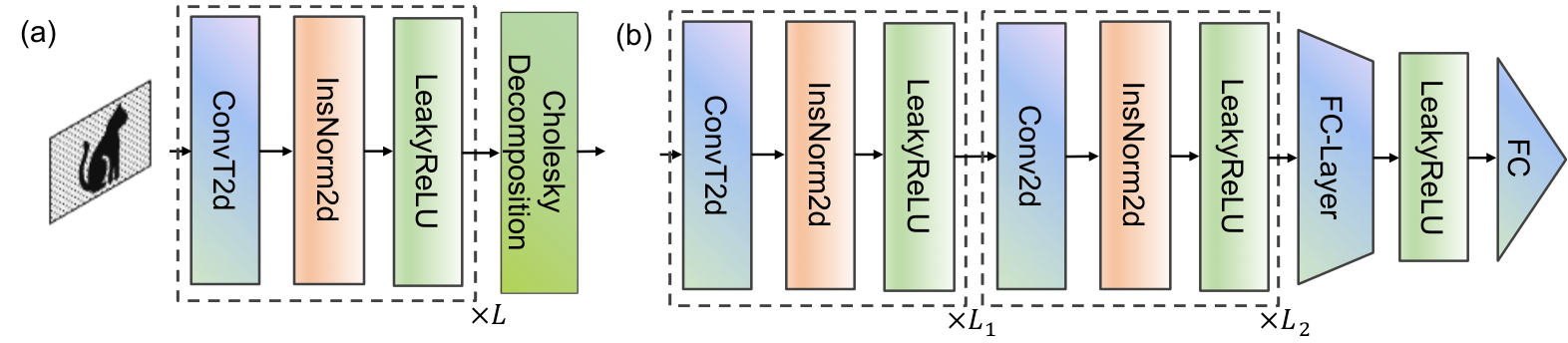
QST. The implementation of ShadowNet in tackling QST is exhibited in Fig. D.5(a). The input data is identical to the one under the attention mechanism, i.e., a reconstructed shadow state is decoupled into a 3d array with the size (an image with pixels and channels). This input is passing through a convolutional block times. Each block contains three components: two-dimensional transposed convolution operator (ConvT2d) zeiler2010deconvolutional, two-dimensional Instance normalization layer (InsNorm2d) ulyanov2016instance, and LeakyReLU activation function. The role of ConvT2d is upsampling the input feature map instead of downsampling, which can increase the spatial resolution of an image. Here we adopt this operation to ensure the same dimension of the input and the final output. Moreover, InsNorm2d is employed to enhance the trainability and stability. After passing convolutional blocks, the output interacts with the Cholesky decomposition layer, restricting the reconstructed state to be physical.
DFE. The implementation of ShadowNet in tackling DFE is exhibited in Fig. D.5(b). Given the input data, a matrix with the size , ShadowNet first applies convolutional blocks to upsample the input feature map. Afterwards, convolutional blocks are applied for the downsampling. The only difference compared to the first blocks is replacing ConvT2d by Convolution operator (Conv2d) to complete downsampling. Subsequently, two fully-connected layers accompanied with LeakyReLU activation function are applied to obtain the final prediction.
SM E More simulation results of ShadowNet
In this section, we provide more simulation details of ShadowNet. Specifically, we first present more results related to the reconstruction of ground state of spin systems in SM E.1. We then showcase more simulation details of ShadowNet when solving DFE tasks in SM E.2. For both tasks, the AdamW optimizer is adopted to update weights of DNN during the training procedure, and the hyper-parameters related to AdamW are kept to be the same. That is, the initial learning rate is and the coefficients used for computing running averages of gradient and its square are default (i.e., 0.9 and 0.99). All numerical simulations are implemented by Julia, PennyLane, and PyTorch frameworks, and trained on four NVIDIA TesLa P40 GPUs.
E.1 Reconstructing ground states of spin systems
Numerical datasets. Here we introduce more information about the datasets exploited in QST tasks. We employ ShadowNet to reconstruct the ground states of two spin systems, i.e., TFIM and XXZ model. For TFIM, the phase of TFIM is ferromagnetic (antiferromagnetic) if (). For XXZ model, it is in the ferromagnetic phase if ; otherwise, it is in the XY phase. For each example, the label (i.e., ground state) and the surrogate quantity (i.e., ground energy) are obtained by the exact diagonalization method, and the data feature (i.e., classical shadows) is obtained by PennyLane bergholm2018pennylane.
Model implementation of ShadowNet under the attention mechanism. We exploit the same ShadowNet under the attention mechanism to complete all tasks related to reconstruct ground states of spin systems. Following the explanations in SM D, we fix the attention block as . The first fully-connected layer maps the input feature from dimensions to dimensions. The dimension of the weight matrices , , and , defined in Eq. (10), is set as .
Predictive faith. The predictive faith of ShadowNet in estimating the ground energy of TFIM and XXZ models can be efficiently derived by using Eq. (20) in SM. C. In the task of reconstructing ground states of TFIM, we have , , and . Let and . When , with probability at least , the estimation error is upper bounded by . When , with probability at least , the estimation error is upper bounded by .
In the task of jointly reconstructing the ground states of TFIM and XXZ models, we further quantify the estimation error of XXZ model and preserve the maximum one. Concretely, we have , , and for all local terms. Let and . When , with probability at least , the estimation error for the ground energy of XXZ model is upper bounded by . As a result, in the joint learning TFIM and XXZ models, the error bound of classical shadows is when .

Performance of ShadowNet under convolutional mechanism. We now apply ShadowNet implemented by convolutional neural network, as explained in SM D.4, to reconstruct the ground states of TFIM and XXZ models. The settings of the constructed dataset are the same with those introduced in the main text. That is, for TFIM, we fix and sample uniformly from the interval to obtain different examples; for XXZ model, we set for and uniformly sample from to generate training and test examples. The training dataset contains the equivalent number of ground states from TFIM and XXZ model. We fix and , and varies the number of training examples as to evaluate the performance of ShadowNet implemented by convolutional neural networks.
The implementation detail of ShadowNet is as follows. The number of encoding block is set as . The kernel size, stride, and padding of ConvT2d in each block are identical, which equal to , , and , respectively. The only difference among convolutional blocks is the number of channels, which is . In the training process, the optimizer, the initial learning rate, the total number of epochs, and the batch size are the same with those introduced in the main text. We repeat the simulation with five times under different random seeds to collect the statistical results.
The simulation results are shown in Fig. E.6. The left panel depicts the performance of ShadowNet implemented by the attention mechanism and the convolution mechanism in the measure of fidelity. After epochs, the averaged fidelity over training examples is near to for the attention mechanism, in both cases of and . However, the averaged fidelity over training examples under the convolutional mechanism is imperfect, which is with and with . In addition, for both attention and convolutional mechanism, ShadowNet experiences the overfitting phenomenon when . By increasing the training example to , this issue can be addressed in which the difference of fidelity between training examples and test examples is ignorable. The right panel shows the performance of ShadowNet implemented by the attention mechanism and the convolution mechanism in the measure of estimation error of the ground state energy. Among different setting, only ShadowNet implemented by the attention mechanism with attains the ignorable estimation error over the test examples.
The distinct learning performance provides the following insights. First, the performance can be effected by the employed architecture of DNN. The inferior performance of the convolutional mechanism compared to the attention mechanism may be caused by its insufficient ability to capture the long-range correlation of data features. In other words, a handcraft architecture of DNN enables the improved learning efficiency of ShadowNet. Second, the number of training examples plays an important role in the performance of ShadowNet. Insufficient training examples may incur overfitting and the unsatisfactory performance of ShadowNet at the inference stage.
E.2 More simulation results in solving direct fidelity estimation tasks
Numerical datasets. In DFE tasks, we apply ShadowNet to predict the fidelity of GHZ states prepared in the ideal and noisy scenarios. The noisy environment is simulated by the local depolarization channel . For the single-qubit state, it mathematical form is . Similarly, for the two-qubit state, it mathematical form is . For each sample, its classical shadows in the noisy scenario and the corresponding labels are collected by PastaQ pastaq, a Julia software toolbox for the simulation of large-qubit quantum circuits.
Model implementation. We use the same ShadowNet under the attention mechanism to tackle all DFE tasks whose implementation is interpreted in SM D. Specifically, the we fix the attention block as . The first fully-connected layer maps the input feature from dimensions to dimensions. The dimension of the weight matrices , , and , defined in Eq. (10), is set as . When the input passes through three attention blocks, the corresponding feature interacts the fully-connected layer with the hidden dimension , followed by the adaptive average pooling and another fully-connected layer with the output dimension .
Predictive faith. We next analyze the predictive faith of ShadowNet under Pauli-based measurements. For an -qubit GHZ state, its Pauli-decomposition yields
where denotes the permutation operator for some permutation . When , the total number of Pauli basis is with for . According to Eq. (22), the estimation error is upper bounded by . This error bound hints that classical shadows with Pauli-based measurement is not a proper choice to evaluate the faithfulness of ShadowNet, due to the large value of the locality .
As emphasized in SM C, Clifford measurements can be exploited in the inference stage to dramatically reduce the estimation error. As proved in huang2020predicting, when (), with probability at least , the estimation error is upper bounded by (). The related numerical results are presented below.
The complementary role of classical shadows and noise parameter. Here we demonstrate more simulation results of ShadowNet under the attention mechanism omitted in the main text. Recall that when applied ShadowNet to solve DFE tasks, the data features incorporate classical shadows and the noisy parameter, whereas the number of measurements of classical shadows is very small (i.e., in learning -qubit GHZ states). A natural question is understanding the role of classical shadows and noise parameters in the task of DFE. That is, whether ShadowNet can effectively learn the mapping rule only using noise parameters or classical shadows as the data features.
To address the aforementioned issue, we conducted simulations with modified datasets, following the setup presented in the main text. In the first modified dataset, we restricted the data feature to include only the noise parameters (i.e., the dimension of each example reduces from to ), while in the second modified dataset, we included only classical shadows in the data features of each example (i.e., the dimension of each example reduces from to ). It is essential to note that apart from the modifications in the datasets, the model implementation and hyper-parameter settings remain exactly identical to those introduced in the main text. Specifically, we apply ShadowNet to solve predict the fidelity between noisy and ideal GHZ states with , where the number of measurements to collect classical shadows is and the size of training examples is .

The simulation results are presented in Fig E.7. While the training loss consistently decreases during optimization for all datasets, we observe that ShadowNet trained on the dataset with full features notably outperforms the other two settings. This advantage is preserved when evaluating the optimized ShadowNet on the test examples, where the average test loss is for the full feature dataset, for the dataset containing only noise parameters, and for the dataset containing only classical shadows. These results pinpoint the complementary role of noise parameters and classical shadows in using ShadowNet to complete DFE tasks.
Numerical results of ShadowNet under convolutional mechanism. Due to the flexible implementation of ShadowNet, we compare the performance of ShadowNet in solving DFE under the mechanism of attention and convolutional mechanism, respectively. The relevant results can provide insights about how the architecture of DNN influences the power of ShadowNet in DFE tasks.
The implementation of ShadowNet with the convolutional mechanism follows the instruction in SM D.4. The construction rule of the dataset is the same with that used in the attention mechanism. The only different is the way to incorporate the local shadows (i.e., a complex three-dimensional array with the size ) and noise parameters (i.e., a real and two-dimensional vector). To accommodate with the architecture of convolutional mechanism, we first append a new dimension to decouple the real and imaginary parts of local shadows, which leads to a four-dimensional array with the size . Then, we duplicate the noise parameter to a matrix, i.e., and append it to the reformulated local shadows. As a result, we obtain the data feature used to train ShadowNet with the size .
To make a fair comparison, we adopt the same hyper-parameter settings and optimization methods with those employed in the main text to train ShadowNet with the convolutional mechanism. We fix , , and . The simulation is repeated with times to collect the statistical results.

The simulation results are shown in Fig. E.8. For both mechanisms, the training and test losses is below after epochs. The achieved results suggest that ShadowNet with the attention and convolutional mechanism can capture the mapping rule from the local shadows and noise parameters to the fidelity between noisy and ideal GHZ states. Moreover, combining the results in Fig. E.7, we can conclude that the construction rule of dataset plays an important role in quantum system learning.
Simulation results under Clifford measurement. The above analysis reflects that classical shadows formed by Pauli-based measurements may not provide a reasonable predictive faith of ShadowNet with few shots, since GHZ state does not have an efficient Pauli decomposition. This issue can be eliminated by random Clifford measurements, as explained in SM C.
We conduct the similar simulation tasks proposed in Ref. huang2020predicting to validate the performance of ShadowNet under the Clifford measurements. Particularly, we focus on the the state preparation error rather than the local depolarization error considered in the main text. In this case, the noisy GHZ state takes the form as
where is the error rate and refers to the orthogonal state and is set as . Let the ideal state be an -qubit . To collect the training and test examples, we randomly sample from to . The noisy state with the varied is randomly measured by Pauli basis with times to form the local shadows as data feature. The corresponding label equals to , which measures the fidelity between and .
The hyper-parameter settings are as follows. We set the number of training examples as , the number of qubit , and the shot number is . The total number of epochs is . The architecture of ShadowNet follows the attention mechanism, which is almost identical to that introduced in SM D. The only modification is the data feature, where the noise parameter is removed. This is because in this noisy scenario, the target label corresponds to the noise parameter . For each setting, we repeat the simulations with five times to collect the statistical results.

The simulation results are shown in Fig. E.9. The training loss after epochs converge to . The discrepancy between the training and test losses is ignorable, implying the generalization ability of ShadowNet. We next employ the trained ShadowNet to understand the predictive faithfulness issue aforementioned. Particularly, we visualize the estimated fidelity of ShadowNet, classical shadows under Clifford and Pauli measurements with shots, and ground truth over test instances in the right panel of Fig. E.9. In this setting, the estimation error of classical shadows under the Clifford measurements is upper bounded by with probability at least 0.8. Despite the large error bound, an interesting phenomenon is that the estimated fidelity generally remains proximal to the ground truth. In other words, a modest number of snapshots allows classical shadows with Clifford measurements to provide a good predictive faith in the average case. Besides, for most instances, ShadowNet outperforms classical shadows with the varied measurement groups, suggesting the effectiveness of ShadowNet.