Quartic Gradient FlowPreprint: RESCEU-16/23

Muzi Hong Email: hong@resceu.s.u-tokyo.ac.jp Affiliation: Research Center for the Early Universe (RESCEU), Graduate School of Science, The University of Tokyo, Tokyo 113-0033, Japan Ryusuke Jinno Email: ryusuke.jinno@resceu.s.u-tokyo.ac.jp Affiliation: Research Center for the Early Universe (RESCEU), Graduate School of Science, The University of Tokyo, Tokyo 113-0033, Japan

August 11, 2026

Abstract

Saddle-point configurations, such as the Euclidean bounce and sphalerons, are known to be difficult to find numerically. In this Letter we study a new method, Quartic Gradient Flow, to search for such configurations. The central idea is to introduce a gradient-flow-like equation in such a way that all the fluctuations around the saddle-point have eigenvalues that are square of the eigenvalues of the original quadratic operator. We illustrate how the method works for the Euclidean bounce and sphalerons.

Introduction. Saddle-point configurations often appear in physics. One of the best known examples is the bounce solution that appears in the calculation of the tunneling rate of false vacuum decay Coleman 1977; Callan and Coleman 1977. Another example is the sphaleron solution Manton 1983; Klinkhamer and Manton 1984 well-known for its important applications in baryogenesis (e.g., Refs. Arnold and McLerran 1987; Kuzmin et al. 1985; Fukugita and Yanagida 1986).

A saddle point has negative mode(s), whereas a minimum has only positive modes. This property of the former can cause problems when one tries to find it numerically. For example, finding multi-field bounces numerically is a non-trivial problem, and a number of approaches have been proposed Claudson et al. 1983; Kusenko 1995; Kusenko et al. 1996; Dasgupta 1997; Moreno et al. 1998; John 1999; Cline et al. 1999a; Cline et al. 1999b; Athron et al. 2019; Konstandin and Huber 2006; Park 2011; Wainwright 2012; Akula et al. 2016; Masoumi et al. 2017; Espinosa 2018; Espinosa and Konstandin 2019; Jinno 2018; Piscopo et al. 2019; Guada et al. 2019; Chigusa et al. 2020; Sato 2020; Sato 2021; Guada et al. 2020. In this context, the gradient flow method, which has been used in various fields of physics to solve differential equations, cannot be used at least naively due to these negative modes. However, a recent proposal Chigusa et al. 2020 showed that the effect of the negative mode(s) can be eliminated by adding an auxiliary term to the flow equation, and thus gradient flow can be used for the search of the bounce (see also Ref. Sato 2020; Sato 2021). The same technique was applied to sphalerons in Ref. Hamada and Kikuchi 2020.

In this Letter, we explore yet another approach for the search of saddle points using gradient flow. We construct a flow equation in such a way that, instead of the original eigenvalues of the fluctuations, their squares appear. As a result, all modes become positive (up to zero modes) and the flow converges to the desired solution. This possibility is also mentioned in the footnote 4 of Ref. Chigusa et al. 2020.

The structure of the Letter is as follows. We introduce the idea in Section 2, and show the numerical results for the calculation of the bounce solutions and sphaleron solutions in Section 3. We discuss future applications and conclude in Section 4.

Central idea. The central idea of this Letter is to introduce a gradient-flow-like equation in such a way that all the fluctuations around the saddle-point solution have positive eigenvalues alone. We illustrate with a single real scalar field, but extension to multi-field is straightforward. We introduce Quartic Gradient Flow as

\displaystyle\partial_{t}\phi+\hat{\cal M}[\phi]\left[\frac{\delta S}{\delta\phi}\right]

\displaystyle=0.

(1)

Here $\hat{\cal M}[\phi]=\delta^{2}S/\delta\phi\delta\phi=-\Delta+\cdots$ , and $\phi=\bar{\phi}+\delta\phi$ denotes the saddle-point solution and a fluctuation around it.

To see how it works, let us expand the equation around the saddle point. The action around the saddle point can be expanded to second order as

\displaystyle S

\displaystyle=\int d^{d}x~\left({\cal L}[\bar{\phi}]+\frac{1}{2}\delta\phi\,\hat{\cal M}[\bar{\phi}]\,\delta\phi+{\cal O}(\delta\phi^{3})\right),

(2)

and thus the flow reduces to

\displaystyle\partial_{t}\phi+\hat{\cal M}^{2}[\bar{\phi}]\delta\phi

\displaystyle\simeq 0.

(3)

We may expand the fluctuation in terms of the eigenfunctions of $\hat{\cal M}[\bar{\phi}]$ as

\displaystyle\delta\phi

\displaystyle=\sum_{n}c_{n}\delta\phi_{n}

(4)

where $c_{1}\leq c_{2}\leq c_{3}\leq\cdots$ is assumed without losing generality, and the $n$ -th eigenfunction and the $n$ -th eigenvalue are denoted as $\delta\phi_{n}$ and $\lambda_{n}$ , respectively. Often there exist negative mode(s) $\lambda_{1}<0$ . The difficulty of naive gradient flow approaches lies in the negativity of this eigenvalue. However, because of the squared operator $\hat{\cal M}^{2}[\bar{\phi}]$ , Quartic Gradient Flow behaves as

\displaystyle\partial_{t}\vec{c}+\Lambda^{2}\vec{c}

\displaystyle\simeq 0,\qquad\Lambda^{2}={\rm diag}(\lambda_{1}^{2},\lambda_{2}^{2},\lambda_{3}^{2},\cdots),

(5)

for the coefficients $\vec{c}=(c_{1},c_{2},c_{3},\cdots)$ . Since the square of a negative value is positive, the flow is expected to converge to the saddle-point solution up to zero-mode directions ¹¹ 1 Note in passing that the Quartic Gradient Flow method can be interpreted as gradient flow to the squared action $S^{\prime}=\int d^{d}x\left(\frac{\delta S}{\delta\phi}\right)^{2}.$ (6) This action has been proposed in Ref. Moreno et al. 1998; John 1999 to find bounce solutions. ²² 2 One might be concerned about the effect of the zero mode(s). Zero modes represent the “directions” along which the system is invariant, and thus $c_{0}$ ’s can take any real value. According to Eq. (5), once $c_{0}$ ’s are fixed by the initial conditions, they do not change as the fictitious time $t$ evolves, and hence they do not spoil our method..

In the following we illustrate how Quartic Gradient Flow works, taking Euclidean bounce and sphalerons as examples. We use forward Euler method to solve the partial differential equations. See the Appendix I for numerical details.

Example 1: single-field Euclidean bounce. We first consider the Euclidean bounce of a single real scalar field in $d$ -dimensions. In this case the functional $S$ is the Euclidean action $S_{E}$ . The bounce configuration is known to be $O(d)$ symmetric, and thus we may write the action as

	$\displaystyle S_{E}$	$\displaystyle=\int d^{d}x~\left[\frac{1}{2}(\partial\phi)^{2}+V(\phi)\right]$
		$\displaystyle=S_{d-1}\int r^{d-1}dr~\left[\frac{1}{2}(\partial_{r}\phi)^{2}+V(\phi)\right].$		(7)

Here the metric is ${\rm diag}(+,+,\cdots)$ in the first line, and $S_{d-1}$ is the surface area of a $(d-1)$ -dimensional unit sphere. The quadratic operator and the Euler-Lagrange equation are

\displaystyle\hat{{\cal M}}[\phi]

\displaystyle=-\partial_{r}^{2}-\frac{d-1}{r}\partial_{r}+V^{\prime\prime}(\phi),

(8)

and

\displaystyle\frac{\delta S_{E}}{\delta\phi}

\displaystyle=-\partial_{r}^{2}\phi-\frac{d-1}{r}\partial_{r}\phi+V^{\prime}(\phi)=0,

(9)

respectively, and thus Quartic Gradient Flow takes the form

\displaystyle\partial_{t}\phi+\left[\partial_{r}^{2}+\frac{d-1}{r}\partial_{r}-V^{\prime\prime}\right]\left[\partial_{r}^{2}\phi+\frac{d-1}{r}\partial_{r}\phi-V^{\prime}\right]

\displaystyle=0.

(10)

The left panel of Fig. 1 shows how the initial configuration (blue) converges to the bounce for an example potential $V(\phi)=m^{2}\phi^{2}/2-a\phi^{3}/3$ with $m=a$ (taken to be unity without loss of generality). For comparison, the black dashed line is the bounce solution calculated with the overshoot-undershoot method. The value $\phi(0)\simeq 4.19$ coincides in both methods.

We may also remove the assumption of $O(d)$ symmetry. In this case, Quartic Gradient Flow becomes

\displaystyle\partial_{t}\phi+\left[\Delta-V^{\prime\prime}(\phi)\right]\left[\Delta\phi-V^{\prime}(\phi)\right]

\displaystyle=0.

(11)

In the right panel of Fig. 1 we use the same potential as before and show how the configuration converges to the saddle point. The value $\phi(x=L/2,y=L/2)\simeq 2.39$ with $L=12$ coincides with the value calculated with the overshoot-undershoot method assuming spherical symmetry in $d=2$ dimensions.

Refer to caption — Figure 1: (Left) Behavior of Quartic Gradient Flow in Example 1 (single-field bounce) for $d=3$ with a spherical symmetric setup. The black dashed line is calculated with the overshoot-undershoot method. (Right) Behavior of Quartic Gradient Flow without assuming spherical symmetry.

Example 2: multi-field Euclidean bounce. We next consider a multi-field case with two real scalar fields. Again the functional $S$ is identified with $S_{E}$ , which we assume to be

\displaystyle S_{E}

\displaystyle=\int d^{d}x~\left[\frac{1}{2}(\partial\phi_{1})^{2}+\frac{1}{2}(\partial\phi_{2})^{2}+V(\phi_{1},\phi_{2})\right].

(12)

Quartic Gradient Flow becomes

\displaystyle\partial_{t}\vec{\phi}+\hat{\cal M}[\vec{\phi}]\left[\frac{\delta S_{E}}{\delta\vec{\phi}}\right]

\displaystyle=0,

(13)

with $\vec{\phi}=(\phi_{1},\phi_{2})^{T}$ and

	$\displaystyle\hat{{\cal M}}[\vec{\phi}]$	$\displaystyle=\left(\begin{array}[]{cc}-\partial_{r}^{2}-\frac{d-1}{r}\partial_{r}+\partial_{\phi_{1}}^{2}V&\partial_{\phi_{1}}\partial_{\phi_{2}}V\\ \partial_{\phi_{1}}\partial_{\phi_{2}}V&-\partial_{r}^{2}-\frac{d-1}{r}\partial_{r}+\partial_{\phi_{2}}^{2}V\end{array}\right),$
	$\displaystyle\frac{\delta S_{E}}{\delta\vec{\phi}}$	$\displaystyle=\left(\begin{array}[]{c}\displaystyle-\partial_{r}^{2}\phi_{1}-\frac{d-1}{r}\partial_{r}\phi_{1}+\partial_{\phi_{1}}V\\[5.69046pt] \displaystyle-\partial_{r}^{2}\phi_{2}-\frac{d-1}{r}\partial_{r}\phi_{2}+\partial_{\phi_{2}}V\end{array}\right).$

For the potential, we use an example in CosmoTransitions Wainwright 2012

	$\displaystyle V(\phi_{1},\phi_{2})$	$\displaystyle=(\phi_{1}^{2}+5\phi_{2}^{2})[5(\phi_{1}-1)^{2}+(\phi_{2}-1)^{2}]$
		$\displaystyle\quad+k\left(\frac{1}{4}\phi_{2}^{4}-\frac{1}{3}\phi_{2}^{3}\right),$		(18)

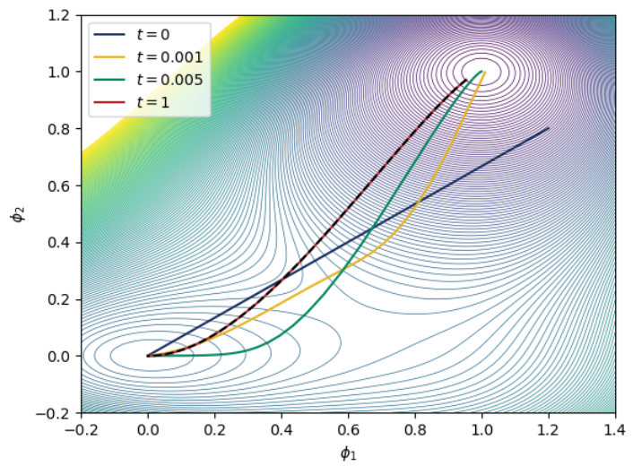
with $k=80$ . The top panel of Fig. 2 shows how Quartic Gradient Flow converges to the bounce solution. The values $\phi_{1}(0)\simeq 0.95$ and $\phi_{2}(0)\simeq 0.97$ coincide with the values calculated with CosmoTransitions ³³ 3 We change the parameter fRatioConv in CosmoTransitions to 0.001 to improve accuracy as in Ref. Chigusa et al. 2020. .

Similarly as Example 1, we may also start without assuming $O(d)$ symmetry. In this case, we can simply use

\displaystyle\hat{{\cal M}}[\phi]

\displaystyle=\left(\begin{array}[]{cc}-\Delta+\partial_{\phi_{1}}^{2}V&\partial_{\phi_{1}}\partial_{\phi_{2}}V\\ \partial_{\phi_{1}}\partial_{\phi_{2}}V&-\Delta+\partial_{\phi_{2}}^{2}V\end{array}\right),

and

\displaystyle\frac{\delta S_{E}}{\delta\vec{\phi}}

\displaystyle=\left(\begin{array}[]{c}-\Delta\phi_{1}+\partial_{\phi_{1}}V\\ -\Delta\phi_{2}+\partial_{\phi_{2}}V\end{array}\right),

in Eq. (13). In the bottom panels of Fig. 2 we show how the configuration converges to the bounce solution. Note that the resulting configuration corresponds to the spherical bounce with $d=2$ . The values $\phi_{1}(x=L/2,y=L/2)\simeq 0.80$ and $\phi_{2}(x=L/2,y=L/2)\simeq 0.79$ with $L=8$ coincide with those calculated with CosmoTransitions setting $d=2$ .

Example 3: sphalerons. We also consider SU(2) sphalerons. Sphalerons are stationary unstable solution of the gauge and Higgs fields. The starting action is

\displaystyle S

\displaystyle=\frac{1}{g^{2}}\int d^{d}x~\left[-\frac{1}{2}{\rm tr}\,F_{\mu\nu}F^{\mu\nu}+|D_{\mu}\Phi|^{2}+V(\Phi)\right],

(23)

and after imposing spherical symmetry and fixing the gauge, the energy becomes (see Appendix II for derivation)

$\displaystyle E=\frac{4\pi}{g^{2}}\int_{0}^{\infty}dr$	$\displaystyle\left[\|\partial_{r}\chi\|^{2}+r^{2}\|\partial_{r}\phi\|^{2}+\frac{1}{2r^{2}}(\|\chi\|^{2}-1)^{2}\right.$
	$\displaystyle\left.+\frac{1}{2}(\|\chi\|^{2}+1)\|\phi\|^{2}-\textrm{Re}(\chi^{*}\phi^{2})\right.$
	$\displaystyle\left.+\frac{\lambda}{g^{2}}r^{2}\left(\|\phi\|^{2}-\frac{1}{2}g^{2}v^{2}\right)^{2}\right],$	(24)

where $\chi$ and $\phi$ are complex fields.

As far as ordinary sphalerons are considered, only the real parts of $\chi$ and $\phi$ take nonzero values Klinkhamer and Manton 1984; Yaffe 1989. Thus, for the purpose of finding the sphaleron solution, we may restrict them to be real and in that case the solution becomes a minimum of the energy (24), not a saddle point. However, since our purpose of studying sphalerons here is to illustrate how Quartic Gradient Flow works in the presence of negative modes, we include the imaginary parts as well in the following analysis. In this case the sphaleron becomes a saddle point of Eq. (24). We also note that the full expression (24) is necessary in finding the most relevant saddle-point solutions for larger $\lambda/g^{2}$ known as bisphalerons Yaffe 1989, though we restrict ourselves to ordinary sphalerons here.

We further redefine $\eta\equiv r\phi$ so that

$\displaystyle E^{\prime}$	$\displaystyle\equiv\frac{g^{2}}{8\pi}E$
	$\displaystyle=\frac{1}{2}\int_{0}^{\infty}dr\left[(\partial_{r}\chi_{r})^{2}+(\partial_{r}\chi_{i})^{2}+(\partial_{r}\eta_{r})^{2}+(\partial_{r}\eta_{i})^{2}\right.$
	$\displaystyle\qquad\qquad\qquad+2U(\chi,\eta;r)\left.\right]+\textrm{const.},$	(25)

with $\chi=\chi_{r}+i\chi_{i}$ , $\eta=\eta_{r}+i\eta_{i}$ , where the constant term comes from integration by parts, and

	$\displaystyle U(\chi,\eta;r)=$	$\displaystyle\frac{1}{4r^{2}}(\|\chi\|^{2}-1)^{2}+\frac{1}{4r^{2}}(\|\chi\|^{2}+1)\|\eta\|^{2}$
		$\displaystyle-\frac{1}{2r^{2}}\textrm{Re}(\chi^{*}\eta^{2})+\frac{\lambda}{2g^{2}r^{2}}\left(\|\eta\|^{2}-\frac{1}{2}g^{2}v^{2}r^{2}\right)^{2}.$		(26)

Then we may use Quartic Gradient Flow for $d=1$ , which takes

\displaystyle\partial_{t}\vec{\phi}+\hat{\cal M}[\phi]\left[\frac{\delta E^{\prime}}{\delta\vec{\phi}}\right]

\displaystyle=0,

(27)

with $\vec{\phi}=(\chi_{r},\chi_{i},\eta_{r},\eta_{i})^{T}$ and

\displaystyle\hat{{\cal M}}[\phi]

\displaystyle=-\left(\begin{array}[]{cccc}\partial_{r}^{2}-\partial_{\chi_{r}}U&-\partial_{\chi_{r}}\partial_{\chi_{i}}U&-\partial_{\chi_{r}}\partial_{\eta_{r}}U&-\partial_{\chi_{r}}\partial_{\eta_{i}}U\\ -\partial_{\chi_{i}}\partial_{\chi_{r}}U&\partial_{r}^{2}-\partial_{\chi_{i}}U&-\partial_{\chi_{i}}\partial_{\eta_{r}}U&-\partial_{\chi_{i}}\partial_{\eta_{i}}U\\ -\partial_{\eta_{r}}\partial_{\chi_{r}}U&-\partial_{\eta_{r}}\partial_{\chi_{i}}U&\partial_{r}^{2}-\partial_{\eta_{r}}U&-\partial_{\eta_{r}}\partial_{\eta_{i}}U\\ -\partial_{\eta_{i}}\partial_{\chi_{r}}U&-\partial_{\eta_{i}}\partial_{\chi_{i}}U&-\partial_{\eta_{i}}\partial_{\eta_{r}}U&\partial_{r}^{2}-\partial_{\eta_{i}}U\end{array}\right),\qquad\frac{\delta E^{\prime}}{\delta\vec{\phi}}=-\left(\begin{array}[]{c}\partial_{r}^{2}\chi_{r}-\partial_{\chi_{r}}U\\ \partial_{r}^{2}\chi_{i}-\partial_{\chi_{i}}U\\ \partial_{r}^{2}\eta_{r}-\partial_{\eta_{r}}U\\ \partial_{r}^{2}\eta_{i}-\partial_{\eta_{i}}U\end{array}\right).

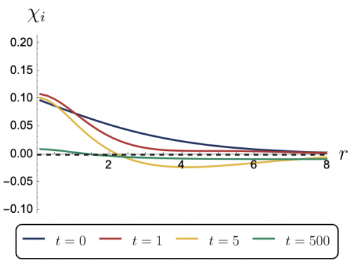
Fig. 3 shows the behavior of the $\chi$ and $\phi$ fields in unit of $gv/\sqrt{2}$ . The colored lines are the time evolution of the fields, while the black dashed lines are the solutions obtained with the numerical method in Ref. Yaffe 1989. We see that the fields converge to the desired sphaleron solution. For the imaginary components, they should eventually converge to zero but there still remain errors of $O(0.01)$ at $t=500$ , possibly because of the finite time and number of grids. In Table 1 we also calculate the sphaleron energy for the converged solutions.

$\lambda/g^{2}$	0.1	0.5	1	5
$E/(m_{W}/\alpha_{W})$	3.60	3.95	4.13	4.56

Table 1: Sphaleron energy

E

calculated with Quartic Gradient Flow, evaluated at

t=500

. The results match those obtained with the numerical method of Ref. Yaffe 1989.

Discussion and Conclusions. In this Letter we study a novel method to calculate saddle-point configurations. The central idea is to introduce a gradient-flow-like equation in such a way that all the fluctuations around the saddle point have positive eigenvalues in the flow equation, Eq. (1). This is made possible by the non-negativity of the eigenvalues of the operator $\hat{\cal M}^{2}[\bar{\phi}]$ around the saddle point, with $\hat{\cal M}[\bar{\phi}]$ being the quadratic operator in the action. The algorithm of Quartic Gradient Flow (1) is simple but powerful: it is applicable to general saddle-point searches without setting up different algorithms for different problems nor finding tailor-made ansatz. We illustrate it with the bounce and sphaleron configurations.

However, we also find several areas for improvement. One of the major ones is the boundary condition. As detailed in the Appendix I, for $O(d)$ bounce solutions we fix the value at the origin by imposing a boundary condition consistent with the original bounce equation (see the text below Eqs. (S1)–(S4)). Without it the configuration would pass through the bounce and reach the trivial solution. Part of the reason for this behavior might be the forward Euler method we use in this Letter. It may cause divergence near the origin in the spherical coordinate when the potential contains terms involving divergent factors such as $\sim 1/r$ . We confirmed that this behavior does not occur if one uses backward Euler method instead. Also, as shown in Fig. 3 for the sphaleron case, the forward Euler method cannot fix the value at the origin. Although one can always use boundary conditions proposed in Refs. Manton 1983; Klinkhamer and Manton 1984; Yaffe 1989 to speculate the field value at the origin, we expect advanced numerical method can calculate the full configuration accurately without additional assumptions.

We present possible future directions from the viewpoint of both numerical methods and physical applications. As mentioned above, explicit numerical methods such as the forward Euler method may bring divergence if the problem involves spherical coordinates. In contrast, implicit methods such as the backward Euler and the Crank-Nicolson methods generally do not lead to such divergence. Implementing the latter methods may allow for convergence of the configuration to the desired solution without some of the boundary conditions imposed in this study. As for physical applications, one may think of various saddle point searches. For example, one could try the method for thin-wall bounce, which we did not consider in this Letter. Sphalerons also have many possible applications. Sphaleron configurations with Chern-Simons number different from $1/2$ , called bisphalerons, are known to appear when $m_{H}^{2}/m_{W}^{2}$ is larger than the Standard Model value Yaffe 1989, and their properties might be investigated with Quartic Gradient Flow. It would also be interesting to study the properties of sphalerons with a finite Weinberg angle, see e.g., Refs. James 1992; Klinkhamer and Laterveer 1992; Kunz et al. 1992. Moreover, other types of sphalerons exist in the Standard Model such as $S^{*}$ and $\hat{S}$ Klinkhamer 1993; Klinkhamer and Rupp 2003. Exploring these configurations using Quartic Gradient Flow would be exciting possibilities, which we leave for future work.

Acknowledgments. The authors are grateful to Yu Hamada, Masazumi Honda, Takeo Moroi, Yutaro Shoji and Hiromasa Watanabe for helpful comments. R. J. is supported by donuts sold in seven-eleven. M. H. is supported by FoPM, WINGS Program, the University of Tokyo and Grant-in-Aid for JSPS Fellows 23KJ0697.

Supplemental Material: Quartic Gradient Flow

I Numerical details

In this Supplemental Material we summarize numerical details to reproduce the results in the Letter.

Example 1: single-field Euclidean bounce. The first example is the single-field bounce. For the case with spherical symmetry, we take $r$ -grid as $r_{i}=(i/n)R$ ( $i=0,1,\cdots,n$ ), and set a mirror at $r_{0}$ such that $\phi_{-1}=\phi_{1}$ and $\phi_{-2}=\phi_{2}$ with $\phi_{i}\equiv\phi(r_{i})$ . We use

$\displaystyle\left[\partial_{r}\phi\right]_{i}$	$\displaystyle=\frac{\phi_{i+1}-\phi_{i-1}}{2\Delta r}+{\cal O}(\Delta r^{2}),$	(S1)
$\displaystyle\left[\partial_{r}^{2}\phi\right]_{i}$	$\displaystyle=\frac{\phi_{i+1}-2\phi_{i}+\phi_{i-1}}{\Delta r^{2}}+{\cal O}(\Delta r^{2}),$	(S2)
$\displaystyle\left[\partial_{r}^{3}\phi\right]_{i}$	$\displaystyle=\frac{\phi_{i+2}-2\phi_{i+1}+2\phi_{i-1}-\phi_{i-2}}{2\Delta r^{3}}+{\cal O}(\Delta r^{2}),$	(S3)
$\displaystyle\left[\partial_{r}^{4}\phi\right]_{i}$	$\displaystyle=\frac{\phi_{i+2}-4\phi_{i+1}+6\phi_{i}-4\phi_{i-1}+\phi_{i-2}}{\Delta r^{4}}+{\cal O}(\Delta r^{2})$	(S4)

as finite difference. We use forward Euler method to obtain the results shown above. Care must be taken for the boundary conditions at $r=0$ . The mirror already fixes $[\partial_{r}\phi]_{0}=[\partial_{r}^{3}\phi]_{0}=0$ . Forward Euler method causes numerical divergence around $r=0$ in this system unless one takes extremely small $\Delta t$ , and hence we calculate $\phi_{0}$ using an additional boundary condition to avoid it. Since the bounce solution behaves as $\phi=\phi_{0}+(1/2d)(\partial V/\partial\phi|_{\phi=\phi_{0}})r^{2}+\cdots$ around $r\sim 0$ , we further impose $[\partial_{r}^{2}\phi]_{0}=(1/d)(\partial V/\partial\phi)_{0}$ at each step to fix the value of $\phi$ at $r=0$ . When calculating $\phi_{0}$ here, we use

\left[\partial_{r}^{2}\phi\right]_{i}=\frac{-\phi_{i+2}+16\phi_{i+1}-30\phi_{i}+16\phi_{i-1}-\phi_{i-2}}{12\Delta r^{2}}+{\cal O}(\Delta r^{4})

(S5)

as finite difference. This means that $\phi_{0}$ is updated according to $\phi_{0}=[32\phi_{1}-2\phi_{2}-12\Delta r^{2}(1/d)(\partial V/\partial\phi)_{0}]/30$ . We observe no significant change in the result for the case of single-field bounce if one uses (S2) to calculate $\phi_{0}$ . However, as elaborated below, the result of multi-field bounce slightly changes, and thus we take (S5) to calculate $\phi_{0}$ . We also impose $\phi_{n}=0$ at each time step. For terms involving $r$ -derivatives of the potential, we do not expand them using the chain rule but rather evaluate $r$ -derivatives directly, e.g. $\partial_{r}V^{\prime}(\phi)=\partial_{r}[(V^{\prime}\circ\phi)(r)]$ . With this setup, the left panel of Fig. 1 is obtained with $d=3$ , $n=200$ , $R=8$ , $\Delta r=0.04$ , and $\Delta t=10^{-7}$ . The initial condition is taken as $\phi_{\rm ini}(r)=10e^{-r^{4}}$ .

We also calculate this case using the backward Euler method, which does not require fixing $\phi$ at $r=0$ with the boundary condition. We first rescale $r$ as in Ref. Chigusa et al. 2020 into $x\in(0,1)$ with $x=\textrm{tanh}(r/R_{0})$ , where we set $R_{0}=6$ . We approximately set $x_{i}=10^{-7}+(i/n)(1-2\times 10^{-7})(i=0,1,\cdots,n)$ . We use the Gaussian elimination method to solve the linear algebraic equations at each time step. When taking $d=3$ , $n=100$ and $\Delta t=10^{-5}$ , one obtains $\phi_{0}\simeq 4.22$ at $t=50$ . As shown in Fig. S1, the configuration first passes through the bounce solution but then comes back and converges to the bounce. The initial condition is taken as $\phi_{\rm ini}(x)=5+6\times 10^{-6}x-30x^{2}+40x^{3}-15x^{4}$ , so that the first derivative of $\phi_{0}=\phi(x=10^{-7})$ and $\phi_{n}=\phi(x=1-10^{-7})$ is zero. We obtain $\phi_{0}\simeq 4.20$ with $n=160$ and other setups unchanged.

For the case without spherical symmetry, we take $xy$ -grid as $x_{i}=(i/n)L$ and $y_{j}=(j/n)L$ ( $i,j=0,1,\cdots,n$ ). We use

$\displaystyle\left[(\partial_{x}^{2}+\partial_{y}^{2})\phi\right]_{i,j}$	$\displaystyle=\frac{\phi_{i+1,j}-2\phi_{i,j}+\phi_{i-1,j}}{\Delta d^{2}}+\frac{\phi_{i,j+1}-2\phi_{i,j}+\phi_{i,j-1}}{\Delta d^{2}}+{\cal O}(\Delta d^{2}),$	(S6)
$\displaystyle\left[(\partial_{x}^{2}+\partial_{y}^{2})^{2}\phi\right]_{i,j}$	$\displaystyle=\frac{\phi_{i+2,j}-4\phi_{i+1,j}+6\phi_{i,j}-4\phi_{i-1,j}+\phi_{i-2,j}}{\Delta d^{4}}+\frac{\phi_{i,j+2}-4\phi_{i,j+1}+6\phi_{i,j}-4\phi_{i,j-1}+\phi_{i,j-2}}{\Delta d^{4}}$
	$\displaystyle+\frac{2(\phi_{i+1,j+1}-2\phi_{i+1,j}+\phi_{i+1,j-1}-2\phi_{i,j+1}+4\phi_{i,j}-2\phi_{i,j-1}+\phi_{i-1,j+1}-2\phi_{i-1,j}+\phi_{i-1,j-1})}{\Delta d^{4}}$
	$\displaystyle+{\cal O}(\Delta d^{2}),$	(S7)

as finite difference. For the boundary condition, we impose $\phi_{i,0}=\phi_{i,n}=\phi_{0,j}=\phi_{n,j}=0$ at each time step. With this setup, the right panel of Fig. 1 is obtained with $n=160$ , $L=16$ , $\Delta d=0.1$ , and $\Delta t=10^{-6}$ . The initial condition is taken as $\phi_{\rm ini}(x,y)=4e^{-[(x-L/2)^{2}+(y-L/2)^{2}]^{2}/16}$ .

Example 2: multi-field Euclidean bounce. For multi-field cases, the procedure is almost the same as single-field cases. Note that, taking two-field cases for instance, cross terms $\partial_{\phi_{1}}\partial_{\phi_{2}}V\times[-\Delta\phi_{2}+\partial_{\phi_{2}}V]$ and $\partial_{\phi_{1}}\partial_{\phi_{2}}V\times[-\Delta\phi_{1}+\partial_{\phi_{1}}V]$ appear in the time evolution of $\phi_{1}$ and $\phi_{2}$ , respectively. With this setup, the top panel of Fig. 2 is obtained with $d=3$ , $n=160$ , $R=8$ , $\Delta r=0.05$ , and $\Delta t=10^{-8}$ . The initial condition is taken as $\phi_{1,{\rm ini}}(r)=1.2e^{-r^{4}/16}$ and $\phi_{2,{\rm ini}}(r)=0.8e^{-r^{4}/16}$ . As mentioned above, if one calculates the field values at origin using (S2) instead of Eq. (S5), one obtains $\phi_{1}(0)\simeq 0.96$ and $\phi_{2}(0)\simeq 0.97$ at $t=5$ with $d=3$ , $n=200$ , $R=8$ , $\Delta r=0.04$ , and $\Delta t=10^{-7}$ . These values deviates by O(1%) from the value obtained with CosmoTransitions. Also, the bottom panels are obtained with $n=80$ , $L=8$ , $\Delta r=0.1$ , and $\Delta t=10^{-6}$ . The initial conditions are taken as $\phi_{1,{\rm ini}}(x,y)=1.2e^{-[(x-L/2)^{2}+(y-L/2)^{2}]^{2}/16}$ and $\phi_{2,{\rm ini}}(x,y)=0.8e^{-[(x-L/2)^{2}+(y-L/2)^{2}]^{2}/16}$ .

Example 3: sphaleron. For the case of sphalerons, we cannot naively use the same update procedure as Example 1, $\phi_{0}=[32\phi_{1}-2\phi_{2}-12\Delta r^{2}(1/d)(\partial U/\partial\phi)_{0}]/30$ (with $d=1$ and $\phi=\chi$ or $\eta$ ), as the potential term contains inverse powers of $r$ . To avoid substituting $r=0$ to the potential, we take $r$ -grid as $r_{i}=((i-1/2)/n)R\ (i=1,\cdots,n)$ , and set a mirror at $r=0$ such that $\phi_{-1}=\phi_{1}$ and $\phi_{-2}=\phi_{2}$ . Note that we do not have $r_{0}$ in this setup and $r_{1}-r_{-1}=R/n$ . We also impose $\eta_{n-1}=2\eta_{n-2}-\eta_{n-3}$ and $\eta_{n}=2\eta_{n-1}-\eta_{n-2}$ at each step, though this does not affect the final result very much. With this setup, Fig. 3 is obtained with $d=1$ , $n=60$ , $R=12$ , $\Delta r=0.2$ , and $\Delta t=10^{-5}$ . The initial condition is taken as $\chi_{r}(r)=-1+2\tanh(r^{2}/16)$ , $\chi_{i}(r)=0.1-0.1\tanh(r/4)$ , $\eta_{r}(r)=r\tanh(r/2)$ , and $\eta_{i}(r)=r(-0.1+0.1\tanh(r/4))$ . When calculating energy given in Table 1, we use

\left[\partial_{r}\phi\right]_{i}=\frac{-\phi_{i+2}+8\phi_{i+1}-8\phi_{i-1}+\phi_{i-2}}{12\Delta r}+{\cal O}(\Delta r^{4})

(S8)

as finite difference to calculate first derivatives. We first calculate the value of $\phi(r)$ from $\phi=\eta/r$ , and use (24) with imaginary fields set to zero to calculate energy.

II The energy of sphalerons

We follow the discussion in Ref. Yaffe 1989 to derive (24). The action of SU(2)-Higgs theory is

S=\frac{1}{g^{2}}\int d^{4}x\left[-\frac{1}{2}\textrm{tr}F_{\mu\nu}F^{\mu\nu}+|D_{\mu}\Phi|^{2}+\frac{\lambda}{g^{2}}\left(\Phi^{\dagger}\Phi-\frac{1}{2}g^{2}v^{2}\right)^{2}\right].

(S9)

The SU(2) gauge field is $A_{\mu}\equiv A^{a}_{\mu}(\tau^{a}/2i)$ , where $\tau^{a}\ (a=1,\ 2,\ 3)$ are the Pauli matrices, and $F_{\mu\nu}\equiv[D_{\mu},D_{\nu}]$ is the SU(2) field strength. $\Phi$ is an SU(2) doublet scalar field with covariant derivative $D_{\mu}\equiv(\partial_{\mu}+A_{\mu})$ . We follow Yaffe’s notation and use $\eta_{\mu\nu}\equiv\textrm{diag}(-,+,+,+)$ in Minkowski spacetime. Here, we neglect U(1)_Y field Klinkhamer and Manton 1984.

When an O(3) rotation of spatial directions can be canceled by a combination of SU(2) gauge and SU(2) global transformations, the field configurations are called “spherically symmetric.” An ansatz for the most general spherically symmetric configuration is given by Refs. Witten 1977; Ratra and Yaffe 1988

$\displaystyle A_{0}(x)$	$\displaystyle=[a_{0}(r,t)\vec{\tau}\cdot\hat{\vec{x}}]/2i,$	(S10)
$\displaystyle A_{j}(x)$	$\displaystyle=\{[\alpha(r,t)-1]e_{j}^{1}/r+\beta(r,t)e_{j}^{2}/r+a_{1}(r,t)e_{j}^{3}\}/2i,$	(S11)
$\displaystyle\Phi(x)$	$\displaystyle=[\mu(r,t)+i\nu(r,t)\vec{\tau}\cdot\hat{\vec{x}}]\xi,$	(S12)

where $\hat{\vec{x}}\equiv\vec{x}/r$ , $r\equiv|\vec{x}|$ , $\alpha(r,t),\beta(r,t),a_{0}(r,t),a_{1}(r,t),\mu(r,t),\nu(r,t)$ are arbitrary real functions and $\xi$ is an arbitrary two-component complex unit vector. $\{e^{k}_{j}\}$ are defined as

$\displaystyle e^{1}_{i}$	$\displaystyle=(\vec{\tau}\cdot\hat{\vec{x}}\tau_{i}-\hat{x}_{i})/i=(\epsilon_{ijk}\hat{x}_{k})\tau_{j},$	(S13)
$\displaystyle e^{2}_{i}$	$\displaystyle=\tau_{i}-\vec{\tau}\cdot\hat{\vec{x}}\hat{x}_{i}=(\delta_{ij}-\hat{x}_{i}\hat{x}_{j})\tau_{j},$	(S14)
$\displaystyle e^{3}_{i}$	$\displaystyle=\vec{\tau}\cdot\hat{\vec{x}}\hat{x}_{i}=(\hat{x}_{i}\hat{x}_{j})\tau_{j}.$	(S15)

$(1+1)$ -dimensional complex fields $\chi\equiv\alpha+i\beta$ , $\phi\equiv\mu+i\nu$ and the $(1+1)$ -dimensional field strength $f_{\mu\nu}=\partial_{\mu}a_{\nu}-\partial_{\nu}a_{\mu}$ with indices $\mu,\nu=0,1$ are defined for convenience. $(1+1)$ -dimensional covariant derivatives are defined as

	$\displaystyle D_{\mu}\chi$	$\displaystyle=(\partial_{\mu}-ia_{\mu})\chi,$		(S16)
	$\displaystyle D_{\mu}\phi$	$\displaystyle=(\partial_{\mu}-ia_{\mu}/2)\phi.$		(S17)

This ansatz is consistent with a U(1) gauge transformation, which is a subgroup of the SU(2) gauge group, consisting of $\{\Omega=\textrm{exp}[i\omega(r,t)\vec{\tau}\cdot\hat{\vec{x}}/2]\}$ . Under these transformations,

$\displaystyle\chi$	$\displaystyle\to e^{i\omega}\chi,$	(S18)
$\displaystyle\phi$	$\displaystyle\to e^{i\omega/2}\phi,$	(S19)
$\displaystyle a_{\mu}$	$\displaystyle\to a_{\mu}+\partial_{\mu}\omega.$	(S20)

The action becomes

	$\displaystyle S=$	$\displaystyle\frac{4\pi}{g^{2}}\int dtdr\left[\frac{1}{4}r^{2}f_{\mu\nu}f^{\mu\nu}+\|D\chi\|^{2}+r^{2}\|D\phi\|^{2}-\textrm{Re}(\chi^{*}\phi^{2})+\frac{1}{2r^{2}}(\|\chi\|^{2}-1)^{2}\right.$		(S21)
		$\displaystyle\left.+\frac{1}{2}(\|\chi\|^{2}+1)\|\phi\|^{2}+\frac{\lambda}{g^{2}}r^{2}\left(\|\phi\|^{2}-\frac{1}{2}g^{2}v^{2}\right)^{2}\right],$		(S22)

using the ansatz given above.

One may first obtain strictly static configurations, which do not depend on time, with gauge fixing $a_{1}=0$ . After gauge transforming them one obtains arbitrary static spherically symmetric field configurations, which are static up to gauge transformations:

$\displaystyle\chi(r,t)$	$\displaystyle=e^{i\omega(r,t)}\bar{\chi}(r),$	(S23)
$\displaystyle\phi(r,t)$	$\displaystyle=e^{i\omega(r,t)/2}\bar{\phi}(r),$	(S24)
$\displaystyle a_{0}(r,t)$	$\displaystyle=\partial_{0}\omega(r,t)+\bar{a_{0}}(r),$	(S25)
$\displaystyle a_{1}(r,t)$	$\displaystyle=\partial_{1}\omega(r,t).$	(S26)

The energy of these static configurations is

	$\displaystyle E=$	$\displaystyle\frac{4\pi}{g^{2}}\int dr\left[\frac{1}{2}r^{2}(\partial_{r}\bar{a}_{0})^{2}+\bar{a}_{0}^{2}\left(\|\bar{\chi}\|^{2}+\frac{1}{4}r^{2}\|\bar{\phi}\|^{2}\right)+\|\partial_{r}\bar{\chi}\|^{2}+r^{2}\|\partial_{r}\bar{\phi}\|^{2}+\frac{1}{2r^{2}}(\|\bar{\chi}\|^{2}-1)^{2}\right.$		(S27)
		$\displaystyle\left.+\frac{1}{2}(\|\bar{\chi}\|^{2}+1)\|\bar{\phi}\|^{2}-\textrm{Re}(\bar{\chi}^{*}\bar{\phi}^{2})+\frac{\lambda}{g^{2}}r^{2}\left(\|\bar{\phi}\|^{2}-\frac{1}{2}g^{2}v^{2}\right)^{2}\right].$		(S28)

One of the field equations yields Gauss’s law

\displaystyle\left(-\partial_{r}r^{2}\partial_{r}+2|\bar{\chi}|^{2}+\frac{1}{2}r^{2}|\bar{\phi}|^{2}\right)\bar{a}_{0}=0.

(S29)

The operator before $\bar{a}_{0}$ is strictly positive, and thus $\bar{a}_{0}$ vanishes, and (24) is obtained with $\bar{\chi}$ , $\bar{\phi}$ replaced by $\chi$ , $\phi$ , respectively.

References

Coleman (1977) S. R. Coleman, Phys. Rev. D 15, 2929 (1977), [Erratum: Phys.Rev.D 16, 1248 (1977)].
Callan and Coleman (1977) C. G. Callan, Jr. and S. R. Coleman, Phys. Rev. D 16, 1762 (1977).
Manton (1983) N. S. Manton, Phys. Rev. D 28, 2019 (1983).
Klinkhamer and Manton (1984) F. R. Klinkhamer and N. S. Manton, Phys. Rev. D 30, 2212 (1984).
Arnold and McLerran (1987) P. B. Arnold and L. D. McLerran, Phys. Rev. D 36, 581 (1987).
Kuzmin et al. (1985) V. A. Kuzmin, V. A. Rubakov, and M. E. Shaposhnikov, Phys. Lett. B 155, 36 (1985).
Fukugita and Yanagida (1986) M. Fukugita and T. Yanagida, Phys. Lett. B 174, 45 (1986).
Claudson et al. (1983) M. Claudson, L. J. Hall, and I. Hinchliffe, Nucl. Phys. B 228, 501 (1983).
Kusenko (1995) A. Kusenko, Phys. Lett. B 358, 51 (1995), eprint hep-ph/9504418.
Kusenko et al. (1996) A. Kusenko, P. Langacker, and G. Segre, Phys. Rev. D 54, 5824 (1996), eprint hep-ph/9602414.
Dasgupta (1997) I. Dasgupta, Phys. Lett. B 394, 116 (1997), eprint hep-ph/9610403.
Moreno et al. (1998) J. M. Moreno, M. Quiros, and M. Seco, Nucl. Phys. B 526, 489 (1998), eprint hep-ph/9801272.
John (1999) P. John, Phys. Lett. B 452, 221 (1999), eprint hep-ph/9810499.
Cline et al. (1999a) J. M. Cline, J. R. Espinosa, G. D. Moore, and A. Riotto, Phys. Rev. D 59, 065014 (1999a), eprint hep-ph/9810261.
Cline et al. (1999b) J. M. Cline, G. D. Moore, and G. Servant, Phys. Rev. D 60, 105035 (1999b), eprint hep-ph/9902220.
Athron et al. (2019) P. Athron, C. Balázs, M. Bardsley, A. Fowlie, D. Harries, and G. White, Comput. Phys. Commun. 244, 448 (2019), eprint 1901.03714.
Konstandin and Huber (2006) T. Konstandin and S. J. Huber, JCAP 06, 021 (2006), eprint hep-ph/0603081.
Park (2011) J.-h. Park, JCAP 02, 023 (2011), eprint 1011.4936.
Wainwright (2012) C. L. Wainwright, Comput. Phys. Commun. 183, 2006 (2012), eprint 1109.4189.
Akula et al. (2016) S. Akula, C. Balázs, and G. A. White, Eur. Phys. J. C 76, 681 (2016), eprint 1608.00008.
Masoumi et al. (2017) A. Masoumi, K. D. Olum, and B. Shlaer, JCAP 01, 051 (2017), eprint 1610.06594.
Espinosa (2018) J. R. Espinosa, JCAP 07, 036 (2018), eprint 1805.03680.
Espinosa and Konstandin (2019) J. R. Espinosa and T. Konstandin, JCAP 01, 051 (2019), eprint 1811.09185.
Jinno (2018) R. Jinno (2018), eprint 1805.12153.
Piscopo et al. (2019) M. L. Piscopo, M. Spannowsky, and P. Waite, Phys. Rev. D 100, 016002 (2019), eprint 1902.05563.
Guada et al. (2019) V. Guada, A. Maiezza, and M. Nemevšek, Phys. Rev. D 99, 056020 (2019), eprint 1803.02227.
Chigusa et al. (2020) S. Chigusa, T. Moroi, and Y. Shoji, Phys. Lett. B 800, 135115 (2020), eprint 1906.10829.
Sato (2020) R. Sato, Phys. Rev. D 101, 016012 (2020), eprint 1907.02417.
Sato (2021) R. Sato, Comput. Phys. Commun. 258, 107566 (2021), eprint 1908.10868.
Guada et al. (2020) V. Guada, M. Nemevšek, and M. Pintar, Comput. Phys. Commun. 256, 107480 (2020), eprint 2002.00881.
Hamada and Kikuchi (2020) Y. Hamada and K. Kikuchi, Phys. Rev. D 101, 096014 (2020), eprint 2003.02070.
Yaffe (1989) L. G. Yaffe, Phys. Rev. D 40, 3463 (1989).
James (1992) M. E. R. James, Z. Phys. C 55, 515 (1992).
Klinkhamer and Laterveer (1992) F. R. Klinkhamer and R. Laterveer, Z. Phys. C 53, 247 (1992).
Kunz et al. (1992) J. Kunz, B. Kleihaus, and Y. Brihaye, Phys. Rev. D 46, 3587 (1992).
Klinkhamer (1993) F. R. Klinkhamer, Nucl. Phys. B 410, 343 (1993), eprint hep-ph/9306295.
Klinkhamer and Rupp (2003) F. R. Klinkhamer and C. Rupp, J. Math. Phys. 44, 3619 (2003), eprint hep-th/0304167.
Witten (1977) E. Witten, Phys. Rev. Lett. 38, 121 (1977).
Ratra and Yaffe (1988) B. Ratra and L. G. Yaffe, Phys. Lett. B 205, 57 (1988).

$\displaystyle E=\frac{4\pi}{g^{2}}\int_{0}^{\infty}dr$	$\displaystyle\left[\|\partial_{r}\chi\|^{2}+r^{2}\|\partial_{r}\phi\|^{2}+\frac{1}{2r^{2}}(\|\chi\|^{2}-1)^{2}\right.$
	$\displaystyle\left.+\frac{1}{2}(\|\chi\|^{2}+1)\|\phi\|^{2}-\textrm{Re}(\chi^{*}\phi^{2})\right.$
	$\displaystyle\left.+\frac{\lambda}{g^{2}}r^{2}\left(\|\phi\|^{2}-\frac{1}{2}g^{2}v^{2}\right)^{2}\right],$	(24)