Matrix Completion over Finite Fields:
Bounds and Belief Propagation Algorithms
Thanks: This work was supported by the Department of Energy under grant DE-SC0022186.
Mahdi Soleymani is with Halıcıoğlu Data Science Institute, University of California San Diego. Qiang Liu is with the State Key Laboratory of Industrial Control Technology, Institute of Cyber-Systems and Control, Zhejiang University,
Hangzhou 310027, China. Hessam Mahdavifar, and Laura Balzano are with the Department of Electrical Engineering and Computer Science, University of Michigan Ann Arbor (e-mail: msoleymani@ucsd.edu, qiangliu_421@zju.edu.cn, hessam@umich.edu, girasole@umich.edu).
Abstract
We consider the low rank matrix completion problem over finite fields. This problem has been extensively studied in the domain of real/complex numbers, however, to the best of authors’ knowledge, there exists merely one efficient algorithm to tackle the problem in the binary field, due to Saunderson et al. [1]. In this paper, we improve upon the theoretical guarantees for the algorithm provided in [1]. Furthermore, we formulate a new graphical model for the matrix completion problem over the finite field of size , , and present a message passing (MP) based approach to solve this problem. The proposed algorithm is the first one for the considered matrix completion problem over finite fields of arbitrary size. Our proposed method has a significantly lower computational complexity, reducing it from in [1] down to (where, the underlying matrix has dimension and denotes its rank), while also improving the performance.
I Introduction
The low rank matrix completion problem aims at recovering the missing entries of a low-rank matrix by observing a small fraction of its entries[2]. This implies that many entries of are redundant and can be discarded for many large-scale scientific computations. This perspective has been used, for example, to speed up tasks in video processing by orders of magnitude [3] by processing only very small subsets of pixels from each frame. There exists an extensive literature studying the low rank matrix completion problem when the underlying matrix is over the field of real/complex numbers, see, e.g., [4]. Moreover, several polynomial-time algorithms exist, including optimization-based methods, that provably recover the underlying real-valued matrices [5][6]. However, such methods can not be applied to the case where the matrix under consideration is over the finite field .
Finite-field matrix completion is, by nature, a different problem compared to the real-field matrix completion, due to the fundamental differences in the underlying algebraic structures of finite fields and the infinite fields of real/complex numbers. The problem has several important applications in network coding [7, 8], index coding [9], and decoding rank-metric codes under erasures [10]. Several prior works [1, 11, 12, 13] have considered rank metric and Hamming metric to establish sample complexity requirements and error bounds in finite-field matrix completion. Another closely related problem is Boolean matrix factorization[14, 15] where the goal is to decompose into the Boolean multiplication of two matrices. The main distinction of our setup compared with this line of work is that the underlying constraints in our model are bilinear constraints over whereas the constraints in [14, 15] involve logical AND/OR operations on Boolean variables.
In this paper, we consider the low rank matrix completion over a finite field . This problem has been proved to be -hard, including the case where the entries are over [16]. A related earlier work [1] showed that the matrix completion problem over can be solved with high probability and proposed a linear programming-based algorithm to tackle this problem. Moreover, [12] proved this problem is fixed-parameter tractable over prime fields. However, efficient algorithms for matrix completion problem over a finite field with arbitrary size do not exist.
The contribution of this paper is twofold. In the first part, we improve upon the theoretical recovery guarantees of the algorithm proposed in [1] for matrix completion over . Specifically, we improve the threshold for the probability of observation of the entries for the algorithm in [1] to successfully recover by making a connection between the probability of unsuccessful recovery in [1] and the error probability of maximum likelihood (ML) decoder for random binary linear codes over the binary erasure channel (BEC). In the second part, we characterize a new graphical model framework for matrix completion over finite fields and utilize a variant of message-passing algorithm to arrive at a solution. Specifically, we run the sum-product algorithm for several rounds repeatedly for a fixed number of iterations, where at the end of each round the value of one randomly picked variable node is fixed. This procedure is continued until we either converge to a solution or the maximum number of rounds is reached. A similar idea is known in the literature as the belief propagation guided decimation (BPGD) approach and has been utilized in the context of the -satisfiability (-SAT) problem [17, 18]. However, the bilinear constraints in our proposed factor graph involve addition and multiplication operations over whereas the constraints in the -SAT problem merely involve logical OR operations. The main distinction between our decimation procedure and the existing ones is that we do not check for any possible contradictions between the variables fixed so far at each intermediate round as it is done in [17, 18] in a subroutine called warning propagation (WP). It turns out that this relaxation does not alter the performance of the algorithm. Our empirical studies demonstrate the superiority of our algorithm over in terms of both the performance and the computational complexity compared to [1].
II Notations
For a and a finite set , is the random subset of obtained by choosing each element of independently with probability . An linear code is a -dimensional subspace of the vector space. The minimum Hamming distance of is denoted by , and the dimension of is also denoted by .The notation denotes an operation similar to inner product over finite field vectors, that is, for we have , where denotes the finite field multiplication. The function nnz returns the number of non-zero elements of its vector/matrix input.
III Matrix Completion over Finite Fields
In this section, we consider the problem of matrix completion over a finite field where we aim at recovering a low-rank matrix based on a partial observation of its entries. Let denote a matrix of rank . Each entry of is revealed by probability , independent of all other entries. Specifically, is observed where . The goal is to fully recover using this partial observation. This problem is known to be NP-hard [19] and, hence, the refined goal is to obtain algorithms that recover with high probability and with polynomial time complexity. This problem has been studied in [1] over and a simple algorithm is provided for the matrix completion over with complexity for , which is polynomial in when is fixed. In this section, we improve the theoretical guarantees on the algorithm provided in [1] modifying their analysis on the probability of recovery error.
The following lemma is used repeatedly in the analysis provided in [1].
Lemma 1
[1, Lemma 1] Let be a binary linear code. If then
| (1) |
Let denote the probability of error under maximum likelihood (ML) decoding over a binary erasure channel (BEC) for an binary linear code. Then, one can observe that
Note that the upper bound provided in Lemma 1 only utilizes the minimum distance of the code and is not tight. In light of this observation, we replace this upper bound with a tighter one for the probability of error of a random binary linear code over BEC. The ensemble of random binary linear codes, denoted by , is obtained by picking each entry of the generator matrix independently and uniformly at random. The average probability of error of a code picked randomly from over BEC under ML decoding is equal to (see, e.g., [20, 21]):
| (2) |
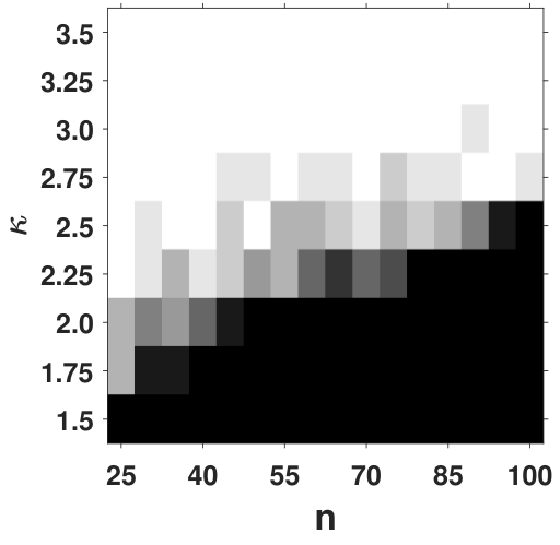
By using the result on the minimum distance of the random binary linear codes [22], we can compare the upper bound provided in (1) with characterized in (2) in Figure 5 in the Appendix. The numerical evaluations, as illustrated in Figure 5 in the Appendix shows a significant gap between the guarantees on characterized in this paper compared to that derived in [1]. This motivates us to determine how this alters the theoretical guarantees on recovering in the matrix completion problem. For the case where the entries are drawn uniformly at random, it is shown in [1] that the proposed algorithm can recover with probability at least when for some that is a function of system parameter and . By following the exact steps in the proofs in [1] and replacing (1) by (2), one can show that the matrix can be recovered for , where . The parameters and are the solutions to
| (3) |
when (1) and (2) are used, respectively (see Appendix A for details). In Figures 3 and 3, we compare the numerical evaluations of and for a certain set of parameters. Note that there exist regions that the analysis in [1] does not provide a non-trivial bound on .
IV A massage passing algorithm for Matrix Factorization over
IV-A Graphical model
Let . Let denote a rank- matrix whose entries are observed according to the observation matrix , i.e., is revealed if and only if , for all and . Note also that for some and since the rank of is . This decomposition is not unique, i.e., there exist several distinct pairs of and such that . Our goal in this section is to find one such pair. Next, we propose a message passing (MP) algorithm to solve this problem.
Figure 3 illustrates the factor graph considered for the matrix factorization problem. Each variable node corresponds to a row in for all . Similarly, each variable node corresponds to a column in for all . If , i.e., the entry of is observed, there exist a factor node with two variable nodes connected to it; and . Note that each factor graph is connected to exactly two variable nodes, where each variable node could be connected to several factor nodes. We regard this problem as a constraint satisfaction problem and leverage the well-known message passing algorithm that attempts to find a solution that satisfies all constraints. Specifically, we use the so-called Sum-Product MP algorithm [23] to compute the marginals of the variable nodes in the factor graph.
Let for and for denote the marginal distributions of and , respectively. Note that there are possibilities for each variable node, i.e., ’s and ’s are tuples with elements. Let and denote the message sent from to and at iteration , respectively. Let also and denote the message sent from and to at iteration , respectively. For all , let denote the set of indices such that , i.e., the indices corresponding to the variable nodes that are connected to the node through a factor node, namely . Similarly, let denote the set of all indices such that . Recall that all the messages are a probability distribution over a set of variables. The -th entry of a vector is denoted by . The Hadamard product between two vectors is a vector consisting of the element-wise product of and , i.e., .
IV-B Message passing algorithm
Let denote a one-to-one mapping from to a the set of vectors of length over . Then, the SP update equations for the message passing algorithm over the factor graph illustrated in Figure 3 under the constraints characterized in (4) can be written as
| (5) | ||||
| (6) | ||||
| (7) | ||||
| (8) |
where denotes equality up to a normalization constant, and denotes the indicator function. Utilizing the SP algorithm to find the marginal distributions of the variable nodes over a factor graph is not new, neither the update equations in (5)-(8). However, we can further simplify equations (5)-(8) and write the update equations for and in terms of and . Note that we only require the final values of and after running the SP algorithm. Therefore, one can re-write the update equations for and as multiplying a certain matrix, as characterized below, by and , respectively. This will significantly reduce the computational complexity of the implementation.
Let denote a matrix whose entry is equal to if , and otherwise. By substituting (7) and (8) into (5) and (6), respectively, one can write
| (9) | |||
| (10) |
where all the vector-vector multiplications are Hadamard multiplication, and, is a one-to-one mapping from to . Recall that all operations are performed over as the belief vectors corresponding to the variable nodes are real-valued.
It is well-known that if the underlying factor graph depicted in Figure 3 is loop-free, then the SP algorithm is nothing but leveraging the distributive law that converges to the true marginals in a finite number of iterations. However, the SP algorithm is also often utilized for loopy factor graphs to approximate the solution. We consider a maximum number of iterations for SP and stop updating the beliefs if the number of iterations reaches this maximum, and the algorithm has not converged yet.
By updating the belief vectors according to the update equations in (5)-(8), some of the multiplications could be computed several times when updating different beliefs. In order to avoid the unnecessary computation overhead, one can bring together all the belief vectors over ’s and ’s into two matrices and multiply them to the constraint matrices once. The resulting matrices’ columns can then be used to update the belief vectors according to (5)-(8). Specifically, let and denote matrices whose columns consist of the beliefs over the variable nodes ’s and ’s at iteration , respectively, i.e.,
| (11) |
and,
| (12) |
and are referred to as belief matrices. Then, one can implement the SP algorithm as provided in Algorithm 1 to obtain an approximation of the marginal distributions of the variable nodes. This modification reduces the computational complexity of updating beliefs according to (9) and (10) by removing the redundant matrix-vector multiplications.


Input: , , , , .
Output: Marginal beliefs and on ’s and ’s.
Initialization: Set and . Set and .
While () () :
| (13) | |||
| (14) |
For and :
| (15) | |||
| (16) |
end;
.
end;
Return: and .
The output of Algorithm 1 does not uniquely determine a solution, neither it captures the correlations between different variable nodes. It merely provides the marginal distributions over ’s and ’s, if it converges. Recall that the LR-factorization is not unique. Therefore the marginal beliefs over the variable nodes capture the likelihood of a certain configuration of variables over the set of all such LR-factorizations consistent with the observation. It is worth noting that, unlike running SP algorithm for the -SAT problem, the SP algorithm over the factor graph depicted in Figure 3 often converges to a solution very fast, but to a trivial one. Specifically, almost all the belief vectors converge to a uniform distribution that includes all possible assignments (except for zero vectors) for ’s and ’s. Roughly speaking, that means running the SP algorithm for a single round does not significantly reduce the size of the search space of the variable nodes, let alone determining them. This motivates us to utilize a decimation procedure that guides us to a solution to the problem which is discussed next.
IV-C Belief propagation-guided decimation algorithm
In order to determine a solution, one can attempt to fix some of the variable nodes based on the associated beliefs returned by Algorithm 1, e.g., by sampling from the corresponding distribution. Since marginal beliefs capture no information about the statistical dependencies between the variable nodes, one might end up with an empty set of feasible solutions after fixing a few variable nodes according to their marginal beliefs. The challenge is that fixing one of the variable nodes alters the beliefs over other nodes through their statistical dependencies, rendering the marginals over other variable nodes incorrect after one variable is fixed by sampling. In order to overcome this problem, we propose utilizing a decimation algorithm that fixes a random variable node at a time and runs the Algorithm 1 again with the modified belief as its initial condition. This procedure is repeated for several rounds until all beliefs converge to single-entry vectors, i.e., the vectors with only one non-zero element, or the maximum number of rounds is reached. In the end, the value of the variable nodes is determined by sampling from the final beliefs. Algorithm 2 describes the steps of this decimation algorithm in detail. By fixing a belief vector, e.g., a column of the belief matrix, we intend to replace it with a one-entry vector having a at a coordinate that is determined by random sampling according to the original vector. In other words, by fixing a belief vector, it collapses to a deterministic distribution with only one non-zero entry (which is equal to ). Algorithm 2 runs in time complexity, provided that and are some constants.
Input: , , , , , .
Output: Completed matrix .
Initialization: Set and , , stop=.
While :
- •
Run Algorithm 1 with and as initial beliefs.
- •
Denote the returned beliefs by and .
- •
Update by fixing all the columns that were fixed during previous steps.
- •
Update by choosing a new column of it that has not been fixed before at random and fix it by sampling.
- •
If (nnz) (nnz): stop= .
- •
Set and , and,
end
Construct and by sampling from the columns of and , respectively.
Return: .
V Experiments
In this section, we compare the performance of Algorithm 2 with that of the algorithm provided in [1] for matrix completion over . Furthermore, we demonstrate the performance of our algorithm over as a proof-of-concept example of a finite field with size larger than .
Figures 4 (a) and (b) illustrate the comparison between the performance of our algorithm and that of the one provided in [1]. The phase-transition plots illustrate the success of the two methods for completing random binary matrices of rank provided that the entries are revealed independently with probability . The random matrix is generated by picking its left and right factor at random, that is, the entries of and are independently drawn from a uniform distribution over . The pixel corresponding to is black if the method fails on all attempts and white if it succeeds on all attempts. The results suggest that our algorithm performs better comparing to the linear programming based approach in [1]. One can observe that when is relatively small, the linear programming based approach is unable to recover the matrix in all trials while our algorithm recovers the matrix with high probability. Note that the computational complexity of Algorithm 2 is while the complexity of the algorithm in [1, Theorem 2] is for completing an matrix. Figure 4 (c) demonstrates the performance of our algorithm over the extension field . It shows that Algorithm 2 recovers the matrix with relatively high probability for a certain range of parameters of the problem. It is worth mentioning that this algorithm is the first efficient algorithm for matrix completion problem over a finite field with a general size, thereby establishing a benchmark for the performance of future algorithms.
References
- [1] J. Saunderson, M. Fazel, and B. Hassibi, “Simple algorithms and guarantees for low rank matrix completion over ,” in 2016 IEEE International Symposium on Information Theory (ISIT). IEEE, 2016, pp. 86–90.
- [2] M. W. Berry, Z. Drmac, and E. R. Jessup, “Matrices, vector spaces, and information retrieval,” SIAM review, vol. 41, no. 2, pp. 335–362, 1999.
- [3] J. He, L. Balzano, and A. Szlam, “Incremental gradient on the Grassmannian for online foreground and background separation in subsampled video,” in 2012 IEEE Conference on Computer Vision and Pattern Recognition. IEEE, 2012, pp. 1568–1575.
- [4] E. Candes and B. Recht, “Exact matrix completion via convex optimization,” Communications of the ACM, vol. 55, no. 6, pp. 111–119, 2012.
- [5] M. A. Davenport and J. Romberg, “An overview of low-rank matrix recovery from incomplete observations,” IEEE Journal of Selected Topics in Signal Processing, vol. 10, no. 4, pp. 608–622, 2016.
- [6] B. Recht, M. Fazel, and P. A. Parrilo, “Guaranteed minimum-rank solutions of linear matrix equations via nuclear norm minimization,” SIAM review, vol. 52, no. 3, pp. 471–501, 2010.
- [7] Y. Birk and T. Kol, “Informed-source coding-on-demand (ISCOD) over broadcast channels,” in Proceedings. IEEE INFOCOM’98, the Conference on Computer Communications. Seventeenth Annual Joint Conference of the IEEE Computer and Communications Societies, vol. 3. IEEE, 1998, pp. 1257–1264.
- [8] E. Byrne and M. Calderini, “Index coding, network coding and broadcast with side-information,” in Network Coding and Subspace Designs. Springer, 2018, pp. 247–293.
- [9] H. Esfahanizadeh, F. Lahouti, and B. Hassibi, “A matrix completion approach to linear index coding problem,” in 2014 IEEE Information Theory Workshop (ITW 2014). IEEE, 2014, pp. 531–535.
- [10] U. Martínez-Peñas, M. Shehadeh, and F. R. Kschischang, “Codes in the sum-rank metric: Fundamentals and applications,” Foundations and Trends® in Communications and Information Theory, vol. 19, no. 5, pp. 814–1031, 2022.
- [11] V. Y. Tan, L. Balzano, and S. C. Draper, “Rank minimization over finite fields: Fundamental limits and coding-theoretic interpretations,” IEEE transactions on information theory, vol. 58, no. 4, pp. 2018–2039, 2011.
- [12] R. Ganian, I. Kanj, S. Ordyniak, and S. Szeider, “Parameterized algorithms for the matrix completion problem,” in International Conference on Machine Learning. PMLR, 2018, pp. 1656–1665.
- [13] S. Vishwanath, “Information theoretic bounds for low-rank matrix completion,” in 2010 IEEE International Symposium on Information Theory. IEEE, 2010, pp. 1508–1512.
- [14] P. Miettinen and S. Neumann, “Recent developments in boolean matrix factorization,” arXiv preprint arXiv:2012.03127, 2020.
- [15] S. Ravanbakhsh, B. Póczos, and R. Greiner, “Boolean matrix factorization and noisy completion via message passing,” in International Conference on Machine Learning. PMLR, 2016, pp. 945–954.
- [16] R. Peeters, “Orthogonal representations over finite fields and the chromatic number of graphs,” Combinatorica, vol. 16, no. 3, pp. 417–431, 1996.
- [17] A. Montanari, F. Ricci-Tersenghi, and G. Semerjian, “Solving constraint satisfaction problems through belief propagation-guided decimation,” arXiv preprint arXiv:0709.1667, 2007.
- [18] M. Mézard, G. Parisi, and R. Zecchina, “Analytic and algorithmic solution of random satisfiability problems,” Science, vol. 297, no. 5582, pp. 812–815, 2002.
- [19] N. J. Harvey, D. R. Karger, and S. Yekhanin, “The complexity of matrix completion,” in Proceedings of the seventeenth annual ACM-SIAM symposium on Discrete algorithm, 2006, pp. 1103–1111.
- [20] M. Soleymani, M. V. Jamali, and H. Mahdavifar, “Coded computing via binary linear codes: Designs and performance limits,” IEEE Journal on Selected Areas in Information Theory, vol. 2, no. 3, pp. 879–892, 2021.
- [21] M. V. Jamali, M. Soleymani, and H. Mahdavifar, “Coded distributed computing: Performance limits and code designs,” in 2019 IEEE Information Theory Workshop (ITW). IEEE, 2019, pp. 1–5.
- [22] A. Barg and G. D. Forney, “Random codes: Minimum distances and error exponents,” IEEE Transactions on Information Theory, vol. 48, no. 9, pp. 2568–2573, 2002.
- [23] F. R. Kschischang, B. J. Frey, and H.-A. Loeliger, “Factor graphs and the sum-product algorithm,” IEEE Transactions on information theory, vol. 47, no. 2, pp. 498–519, 2001.
- [24] J. T. Parker, P. Schniter, and V. Cevher, “Bilinear generalized approximate message passing-part I: Derivation,” IEEE Transactions on Signal Processing, vol. 62, no. 22, pp. 5839–5853, 2014.
- [25] ——, “Bilinear generalized approximate message passing-part II: Applications,” IEEE Transactions on Signal Processing, vol. 62, no. 22, pp. 5854–5867, 2014.
Appendix A Derivation of (19) as described in [1]
The meta algorithms proposed in [1] for matrix completion are all of the following form for different choices of and .
1) Construct and
2) For construct with columns that are a basis for span .
3) Return for all satisfying
Let (for ) and let . We say that and are consistent with if
| (17) | ||||
If, in addition, (17) consists of a single point we say that and are uniquely consistent with .
It was showed that if is a subspace of dimension . Then
Therefore, if we set , and if both of and occur, then and are consistent with . And if and are uniquely consistent with , then they can recover the matrix successfully with high probability.
The way to construct and is the following algorithm.
Input: , positive integer
1:
2: for do
3:
4: if for all then
5:
6: end if
7: end for
Step1: Prove that and are consistent with with probability at least .Where we set .
If we fix then since any if and only if for all . Let . Suppose , or equivalently that . Then the probability that (i.e. ) is bounded above by .
Taking a union bound over all with , the probability that is at most
| (18) | ||||
Similarly, span with probability at most . Take a union bound with this two events, we can get that for , where , and are consistent with with probability more than . The parameters and are the solutions to
| (19) |
Step2 Prove that and are uniquely consistent with with probability at least .