Quantum tasks assisted by quantum noise

Our operational definition of a quantum task $Q$ will be any sequence of unitary gates and projective measurements applied to some (pure) quantum state $|\psi\rangle\in\mathcal{H}$, where $\mathcal{H}$ denotes the set of possible resource states. We will further assume that the effectiveness of the state $|\psi\rangle$ for performing the task $Q$ is quantified by a real-valued function $u:\mathcal{H}\to\mathbb{R}$, which we call the “utility function” for the task $Q$. We emphasize that $u$ can be any measurable function of the state $|\psi\rangle$ whatsoever. (Thus $u$ is less constrained than the analogous notion of “resource measure” in quantum resource theoriesChitambar and Gour 2019.)

Let us now suppose that $|\psi\rangle$ exhibits quantum noise; to be precise, suppose that $|\psi\rangle$ is drawn from some random ensemble of pure states $\mathcal{E}$. Then, letting $\mathbb{E}$ denote expectation values over the ensemble $\mathcal{E}$, we define the “expected utility” for the ensemble $\mathcal{E}$ to be the number

We note that according to this formulation of expected utility, $u$ will generally already encode a Born-rule average over possible outcomes of projective measurements on the state $|\psi\rangle$. The average $\mathbb{E}$ thus represents an additional average over noisy quantum states $|\psi\rangle$. The resulting definition of $U$ in Eq. (1) seems to us the most simple-minded way of combining these two averages. However, just as for the notion of expected utility in economic theoryVon Neumann and Morgenstern 2007, this should be regarded as a convenient choice rather than a canonical definition, and it is conceivable that for more elaborate quantum tasks involving post-selection or feedback based on measurement outcomes, an alternative definition of $U$ will be more useful.

As a more structured example that is germane to our considerations below, suppose that $|\psi\rangle$ depends smoothly on $M$ real parameters $g_{1},g_{2},\ldots,g_{M}$, and that the ensemble $\mathcal{E}$ is defined by randomness in these couplings $\mathbf{g}\in\mathbb{R}^{M}$. (For example, $|\psi\rangle$ might be the ground state of a disordered Hamiltonian with $M$ random couplings.) Then we can treat $u$ as a function $u:\mathbb{R}^{M}\to\mathbb{R}$ and by Jensen’s inequalityADi 2008 it follows that

as a function of $\mathbf{g}$. Thus if $u(\mathbf{g})$ is a convex function, disorder in $\mathbf{g}$ will never decrease the expected utility of the quantum task $Q$. In this way, quantum noise can enhance the expected utility of a quantum task.

At the same time, the “global” condition that $u(\mathbf{g})$ is convex is rather restrictive and too strong to be satisfied by realistic examples, including the main example of interest below. Let us therefore, following PrattPratt 1964, consider the case of perturbatively weak randomness, with $\mathbf{g}=\bar{\mathbf{g}}+\delta\mathbf{g}$, where the $\delta g_{i}$ are possibly correlated random variables, with zero mean $\mathbb{E}[\delta\mathbf{g}]=0$, covariance $C_{ij}=\mathbb{E}[\delta g_{i}\delta g_{j}]=\mathcal{O}(\sigma^{2})$ where $\sigma\ll 1$, and suppose that all higher moments of $\delta\mathbf{g}$ are $\mathcal{O}(\sigma^{3})$ as $\sigma\to 0$. We additionally assume that $u(\mathbf{g})$ is thrice differentiable. Then by Taylor’s theorem it is immediate that

as $\sigma\to 0$, where we introduced the Hessian

It is clear that the effect of small random perturbations $\delta\mathbf{g}$ is controlled by the spectrum of the Hessian $H(\bar{\mathbf{g}})$; if the latter is positive (resp. negative) definite, such perturbations will always increase (resp. decrease) the expected utility of $Q$. For a general covariance matrix $C$, this is the most general “local” condition that will guarantee a definite sign for the second variation

However, if the covariance matrix has additional structure, then weaker conditions will suffice.

For example, in the specific case of i.i.d. zero-mean noise, which we can write as $C_{ij}=\sigma^{2}\delta_{ij}$, Eq. (3) simplifies to

so that a sufficiently small and nonzero amount of uncorrelated noise will always be helpful for accomplishing the quantum task $Q$ provided that $\nabla^{2}u(\bar{\mathbf{g}})>0$. Thus we have identified three increasingly weak conditions under which disorder will always increase (resp. decrease) the expected utility of $Q$.

Finally, let us suppose that the agents executing the quantum task $Q$ in question are free to choose the quantum noise level $\sigma\ll 1$ for their experimental system. Then, borrowing standard economic terminologyPratt 1964, economically rational agents seeking to maximize their joint expected utility $u$ will be either “risk-seeking” or “risk-averse” depending on whether the sign of $\delta u^{(2)}$ is positive or negative.

We now discuss a specific realization of the theory presented above in the context of the parity gameMermin 1990; Brassard et al. 2005b. We first briefly recall some key properties of this gameBrassard et al. 2005a; Bulchandani et al. 2023a, so as to be self-contained.

Each round of the parity game can be played by $N\geq 3$ players and a referee. At the beginning of the game, the referee gives the $j$th player a classical bit $a_{j}\in\{0,1\}$. The bit string $\vec{a}=(a_{1},a_{2},\ldots,a_{N})$ is drawn uniformly randomly from the set of $2^{N-1}$ bit strings satisfying the promise $\sum_{j=1}^{N}a_{j}\mod 2=0$. The players may not communicate classically with one another during the course of the game, and to win the game, they must each return a classical bit $b_{j}\in\{0,1\}$ to the referee. The players collectively win the game if

and lose the game otherwise. It can be shown that a set of purely classical players win the game with a probability at most

and that there exist classical strategies saturating this boundBrassard et al. 2005b.

On the other hand, a set of quantum players who share the $N$-qubit GHZ state $|\psi\rangle=|\mathrm{GHZ}^{+}\rangle$ before playing the game, where

can win the game with probability one. In order to achieve this, the players apply the BBT protocol of gates and measurement $\mathcal{P}_{\mathrm{BBT}}$ to their shared state $|\psi\rangle$, defined as follows: First, each player acts on their qubit with an input-dependent phase gate,

Second, each player rotates their basis to the $\hat{X}$ or Hadamard basis by applying the unitary

Finally, each player measures their qubit in the $\hat{Z}$ basis, yielding a measurement outcome $(-1)^{b_{j}}$, and returns the bit $b_{j}$. We refer to MerminMermin 1990 and BBTBrassard et al. 2005b for an explanation of why this quantum strategy always wins the game.

In previous workBulchandani et al. 2023a, we generalized the BBT protocol to arbitary states $|\psi\rangle$ by considering the quantum strategy $\mathcal{S}=(|\psi\rangle,\mathcal{P}_{\mathrm{BBT}})$ for playing the parity game, which consisted of applying the input-dependent protocol $\mathcal{P}_{\mathrm{BBT}}$ to an arbitrary pure state $|\psi\rangle$. There we found the explicit formula

for the quantum probability of winning the game, which attains its maximum for the GHZ state $|\psi\rangle=|\mathrm{GHZ}^{+}\rangle$. This result can be seen as a simplified but practically useful form of the full “rigidity” statement for the parity game Werner and Wolf 2001; Colbeck 2011; McKague 2010; Miller and Shi 2013.

For example, in previous work we computed Eq. (12) exactly for the $g>0$ ground state of the transverse-field Ising model

on a ring with $j\equiv j+N$, finding the expressionsBulchandani et al. 2023a¹¹ 1 The last line corrects a stray factor of two in a previously published formulaBulchandani et al. 2023a.

with the allowed wavenumbers $k$ defined by

where $\tan{\theta_{k}(g)}=\sin{k}/(g-\cos{k})$ and it will be useful to define $\epsilon_{k}(g)=\sqrt{1+g^{2}-2g\cos k}$ (see discussion around Eq. (44) for further details). We found that for all $0<g<1.506\ldots$, this quantum strategy exhibited a weak quantum advantage relative to the optimal classical probability of winning $p_{\mathrm{cl}}^{*}$, i.e. $\Delta p=p_{\mathrm{qu}}(g)-p_{\mathrm{cl}}^{*}$ was positive but exponentially small in $N$, with both $p_{\mathrm{qu}}(g)$ and $p_{\mathrm{cl}}^{*}$ themselves exponentially small corrections to the winning probability for random guessing, $p_{\mathrm{r}}=1/2$. We previously referred to this competition as a “battle of exponentials” between the exponentially small differences $p_{\mathrm{qu}}(g)-p_{\mathrm{r}}$ and $p_{\mathrm{cl}}^{*}-p_{\mathrm{r}}$ .

The question now arises of how best to define the collective utility of a set of players of a nonlocal game. We emphasize from the beginning that this choice is arbitrary; as a simple example, if the players collectively receive a payoff $1$ whenever they win the game and a payoff $0$ whenever they lose the game, their expected payoff (the standard notion of utility for gamesVon Neumann and Morgenstern 2007) recovers the quantum probability of winning. Thus for the parity game and the strategy $\mathcal{S}=(|\psi\rangle,\mathcal{P}_{\rm BBT})$, this definition yields the utility function

An undesirable property of this utility function is that it does not usefully capture the quantum advantage of the players relative to a set of purely classical players. A naive modification of this quantity is $u(|\psi\rangle)=\Delta p=p_{\mathrm{qu}}-p_{\mathrm{cl}}^{*}$, which has the convenient property that it is only positive if the strategy $\mathcal{S}$ yields a quantum advantage for the parity game. However, the exponential smallness of this quantity makes it unsuitable for directly probing weak quantum advantage as arises quite generically for physically realistic even-parity statesBulchandani et al. 2023a. From this viewpoint, a “useful” measure of weak quantum advantage is one that quantifies the rate of decay of this exponential with the number of players, compared to the classical probability of winning, leading us to the definition

which we shall adopt throughout the remainder of this work. We emphasize that this formula can be applied to any nonlocal game and quantum strategy with $p_{\mathrm{qu}}>p_{\mathrm{r}}$ (there is no point in considering strategies that perform worse than random guessing). We note that when the quantum strategy $\mathcal{S}$ is optimal, the quantities $2\Delta p$ and $(p_{\mathrm{qu}}-p_{r})/(p^{*}_{\mathrm{cl}}-p_{r})$ are known as the “bias difference" and the “bias ratio" respectively Bene Watts et al. 2018; in this language, our preferred notion of utility for suboptimal quantum strategies $\mathcal{S}$ is the logarithm of a suboptimal bias ratio.

For the parity game and the quantum strategy $\mathcal{S}=(|\psi\rangle,\mathcal{P}_{\mathrm{BBT}})$, where $|\psi\rangle$ has even parity $\prod_{j=1}^{N}\hat{X}_{j}|\psi\rangle=|\psi\rangle$, this formula reduces to

so that

According to our terminology of strong and weak quantum advantage, the quantum strategy $\mathcal{S}$ can only exhibit either of these properties if the limit

exists and is strictly positive. The special case

corresponds to strong quantum advantage for the parity game, while all other cases

correspond to weak quantum advantage.

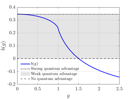
For the specific case that $|\psi(g)\rangle$ is a ground state of the transverse-field Ising model with coupling strength $g>0$, Eq. (14) implies that the utility Eq. (17) of the transverse-field Ising ground state for playing the parity game is given by

where

which is monotonically decreasing with a unique zero $b(g_{*})=0$ at $g_{*}=1.506...$. This function is plotted in Fig 1.

Thus the transverse-field Ising ground state can provide strong quantum advantage (as $g\to 0^{+}$), weak quantum advantage (for $0<g<g_{*}$) or no quantum advantage (for $g\geq g_{*}$) for the parity game, depending on the value of the coupling strength $g>0$.

The simplest limit to consider is perfectly correlated disorder, with $g_{1}=g_{2}=\ldots=g_{N}=g$ and $g>0$ drawn from some probability distribution with small variance $\sigma^{2}\ll 1$. In this case, we have

Thus to determine the perturbative effect of disorder it suffices to compute

From Eq. (28), we find that

and

where we defined

The rescaled second variation $\delta u^{(2)}$ in this case is given by

Eq. (34) is plotted in Fig. 2. A striking conclusion from this plot is that rational players will prefer weak disorder in the paramagnetic phase, because it enhances their expected probability of winning. Meanwhile, they will avoid weak disorder in the ferromagnetic phase, because this diminishes their expected probability of winning. In the large-system limit²² 2 Note that one cannot take the ordinary thermodynamic limit, because spontaneous symmetry breaking tends to eliminate quantum advantage for nonlocal gamesBulchandani et al. 2023a. as $N\to\infty$, these two regimes are cleanly separated by a divergence in the rescaled second variation that lies precisely at the Ising critical point $g=g_{c}=1$. A more detailed asymptotic analysis reveals that this divergence is independent of the order of limits: the rescaled second variation diverges whether one lets $g\to g_{c}$ having already taken the large-system limit as $N\to\infty$, or lets $N\to\infty$ while holding $g=g_{c}$ fixed (see Appendix C).

We next consider the case of i.i.d. couplings $g_{i}$ drawn from a distribution with $\sigma\ll\bar{g}$, so that $\delta g_{i}=g_{i}-\bar{g}$ satisfies

Then by Eq. (6) we have

and

(see Appendix B for details). This formula is verified against numerical simulations in Fig. 3.

The behaviour of the rescaled second variation

as $N\to\infty$ is depicted for a wider range of values of the mean transverse-field strength $\bar{g}$ in Fig. 4. As for the case of perfectly correlated disorder, we find that rational players will eschew disorder in most (>$99\%$) of the ferromagnetic phase and prefer disorder in the paramagnetic phase, since the Laplacian is negative (resp. positive) in these two regimes. Similarly, the Laplacian diverges at the Ising critical point $g=g_{c}$. However, in contrast to the perfectly correlated case, the Laplacian changes sign at a value of $g$ that differs from the Ising critical point, $g\approx 0.9902<g_{c}$ in the large-system limit. We obtain this value by approximating the sum Eq. (37) by an integral, which we evaluate numerically; this integral yields the blue dashed line in Fig. 4.

To clarify the meaning and significance of these results, it is helpful to study the histograms of $u(\mathbf{g})-u(\bar{\mathbf{g}})$ while keeping $\sigma$ fixed and varying the number of qubits $N$. Such histograms are depicted in Fig. 5. Quite strikingly, we see that as $N$ is varied, there is an extensive shift in the expected utility corresponding to extensivity of $\nabla^{2}u(\bar{\mathbf{g}})$, which can be deduced from Eq. (37). According to Mermin’s formulation of the parity gameMermin 1990, this can be interpreted as an exponentially large change in the average number of satisfied GHZ stabilizers for the state $|\psi(\mathbf{g})\rangle$. Following our discussion in the previous section, this change can be negative (deep in the ferromagnetic phase) or positive (deep in the paramagnetic phase). In the paramagnetic phase, the lower panel of Fig. 5 demonstrates an even more dramatic effect that can occur for certain parameter values, whereby the introduction of disorder tips the system from a regime of no quantum advantage to a regime of weak quantum advantage for the parity game. We have chosen to illustrate this effect away from the immediate vicinity of $g_{*}$ where the change in $b$ is relatively weak; by moving $\bar{g}$ closer to $g_{*}$, this effect can be amplified. For example, at $\bar{g}=1.55$, with the same system size and disorder distribution, we find that $b(\bar{\mathbf{g}})=-0.010...<0$ while $\mathbb{E}[b(\mathbf{g})]=0.015...>0$, so that the disorder-averaged value of $b$ is roughly an order of magnitude larger than for the example depicted in Fig. 5.

Finally, we note that the shape of the distributions of $u(\mathbf{g})$ becomes qualitatively normal as $N$ increases, which is consistent with the intuition that the quantum winning probability for the RTFIM ground state effectively computes the determinant of a large random matrix (see Eq. (67)), and should therefore be asymptotically lognormally distributed as $N\to\infty$.

In Sections III.1 and III.2 above, we considered the limits of perfectly correlated and perfectly uncorrelated disorder in the random transverse-field Ising model. We finally turn to the intermediate and physically relevant case of disorder with a finite correlation length $\xi$. Thus we suppose that the small random perturbations $\{\delta g_{j}\}$ satisfy

with $\sigma\ll 1$. In order to probe the effect of the correlation length on the expected utility, we again consider the rescaled second variation of the expected utility $\frac{\delta u^{(2)}(\mathbf{g})}{N\sigma^{2}}$, with $\delta u^{(2)}$ obtained exactly from Eq. (82). We find that for a fixed system size $N$, this interpolates smoothly between the behaviours identified above in the limits of perfectly correlated and perfectly uncorrelated disorder, as shown in Figure 6.

We can gain some insight into this behaviour through the following intuitive argument; if $\xi=\mathcal{O}(N^{0})$ (the most physical case) then the system will resemble the limit of perfectly uncorrelated disorder on length scales $\gg\xi$ as $N\to\infty$, and should thus recover the qualitative behaviour observed in Sec. III.2. Conversely, if $\xi$ grows faster than $N$, e.g. as $\xi=N^{2}$, then the separation of scales $N\ll\xi$ implies that the disorder will appear perfectly correlated at the system length scale $N$, recovering the qualitative behaviour observed in III.1. These intuitions are consistent with the behaviour observed in Fig. 6 and with numerical simulations for multiple values of $N$ (not shown), and can be justified more systematically from Eq. (5).

References

- Daniel and Miyake (2021) A. K. Daniel and A. Miyake, Physical Review Letters 126 (2021), URL https://doi.org/10.1103%2Fphysrevlett.126.090505.
- Daniel et al. (2022) A. K. Daniel, Y. Zhu, C. H. Alderete, V. Buchemmavari, A. M. Green, N. H. Nguyen, T. G. Thurtell, A. Zhao, N. M. Linke, and A. Miyake, Physical Review Research 4, 033068 (2022).
- Bulchandani et al. (2023a) V. B. Bulchandani, F. J. Burnell, and S. L. Sondhi, Physical Review B 107 (2023a), URL https://doi.org/10.1103%2Fphysrevb.107.045412.
- Bulchandani et al. (2023b) V. B. Bulchandani, F. J. Burnell, and S. L. Sondhi, Phys. Rev. B 107, 035409 (2023b), URL https://link.aps.org/doi/10.1103/PhysRevB.107.035409.
- Brassard et al. (2005a) G. Brassard, A. Broadbent, and A. Tapp, Foundations of Physics 35, 1877 (2005a), ISSN 1572-9516, URL https://doi.org/10.1007/s10701-005-7353-4.
- Abramsky et al. (2017) S. Abramsky, R. S. Barbosa, and S. Mansfield, Phys. Rev. Lett. 119, 050504 (2017), URL https://link.aps.org/doi/10.1103/PhysRevLett.119.050504.
- Cabello (2021) A. Cabello, Physical Review Letters 127, 070401 (2021).
- Raussendorf (2013) R. Raussendorf, Phys. Rev. A 88, 022322 (2013), URL https://link.aps.org/doi/10.1103/PhysRevA.88.022322.
- Howard et al. (2014) M. Howard, J. Wallman, V. Veitch, and J. Emerson, Nature 510, 351 (2014).
- Van den Nest (2013) M. Van den Nest, Phys. Rev. Lett. 110, 060504 (2013), URL https://link.aps.org/doi/10.1103/PhysRevLett.110.060504.
- Chen et al. (2022) J. Chen, E. Stoudenmire, and S. R. White, arXiv preprint arXiv:2210.08468 (2022).
- Von Neumann and Morgenstern (2007) J. Von Neumann and O. Morgenstern, in Theory of games and economic behavior (Princeton university press, 2007).
- Pratt (1964) J. W. Pratt, Econometrica 32, 122 (1964).
- Fialík (2010) I. Fialík, arXiv preprint arXiv:1006.1411 (2010).
- Brassard et al. (2005b) G. Brassard, A. Broadbent, and A. Tapp, Recasting Mermin’s multi-player game into the framework of pseudo-telepathy (2005b), eprint quant-ph/0408052.
- Mermin (1990) N. D. Mermin, Physical Review Letters 65, 1838 (1990).
- Gill (1977) J. Gill, SIAM Journal on Computing 6, 675 (1977), eprint https://doi.org/10.1137/0206049, URL https://doi.org/10.1137/0206049.
- Arrow (1964) K. J. Arrow, The review of economic studies 31, 91 (1964).
- Chitambar and Gour (2019) E. Chitambar and G. Gour, Reviews of Modern Physics 91 (2019), URL https://doi.org/10.1103%2Frevmodphys.91.025001.
- ADi (2008) A Dictionary of Statistics (Oxford University Press, 2008), ISBN 9780191726866, URL https://www.oxfordreference.com/view/10.1093/acref/9780199541454.001.0001/acref-9780199541454.
- Werner and Wolf (2001) R. F. Werner and M. M. Wolf, Physical Review A 64 (2001), URL https://doi.org/10.1103%2Fphysreva.64.032112.
- Colbeck (2011) R. Colbeck, Quantum and relativistic protocols for secure multi-party computation (2011), eprint 0911.3814.
- McKague (2010) M. McKague, Self-testing graph states (2010), eprint 1010.1989.
- Miller and Shi (2013) C. A. Miller and Y. Shi, Optimal robust quantum self-testing by binary nonlocal xor games (2013), eprint 1207.1819.
- Bene Watts et al. (2018) A. Bene Watts, A. W. Harrow, G. Kanwar, and A. Natarajan (2018), URL http://drops.dagstuhl.de/opus/volltexte/2018/10103/.
- Mbeng et al. (2020) G. B. Mbeng, A. Russomanno, and G. E. Santoro, The quantum ising chain for beginners (2020), eprint 2009.09208.
- Preskill (2018) J. Preskill, Quantum 2, 79 (2018), URL https://doi.org/10.22331%2Fq-2018-08-06-79.
- Aharonov et al. (2023) D. Aharonov, X. Gao, Z. Landau, Y. Liu, and U. Vazirani, in Proceedings of the 55th Annual ACM Symposium on Theory of Computing (ACM, 2023), URL https://doi.org/10.1145%2F3564246.3585234.
- Du et al. (2021) Y. Du, M.-H. Hsieh, T. Liu, D. Tao, and N. Liu, Physical Review Research 3 (2021), URL https://doi.org/10.1103%2Fphysrevresearch.3.023153.
- Domingo et al. (2023) L. Domingo, G. Carlo, and F. Borondo, Scientific Reports 13, 8790 (2023).
- Damski and Rams (2013) B. Damski and M. M. Rams, Journal of Physics A: Mathematical and Theoretical 47, 025303 (2013), URL https://doi.org/10.1088%2F1751-8113%2F47%2F2%2F025303.
Appendix A Quantum probability of winning the parity game with random transverse-field Ising ground states
In this Appendix, we show how to compute the quantum probability of winning the parity game with the quantum strategy , Eq. (12), where is the ground state of the random transverse-field Ising model Eq. (25).
A.1 Conventions for TFIM diagonalization
Since we will need them later, we first fix conventions for the standard diagonalization of the clean TFIM Eq. (13) via Jordan-Wigner transformation to free fermions Damski and Rams 2013; Mbeng et al. 2020. For simplicity, we will always assume periodic boundary conditions for the spin degrees of freedom.
The Jordan-Wigner transformation is