High-Order Numerical Integration on Domains Bounded by Intersecting Level Sets

The general idea is to simplify the domain of the integral by transforming it into a hypercube. In case of the volume integral (1), we map a hypercube $C=[-1,1]^{3}$ to $\Omega$ with a mapping $T$,

encoding $\Omega$’s geometry in the Jacobian determinant $|\text{det}(DT(\tilde{x}))|=J(T(\tilde{x}))$,

Since it is a cartesian product of intervals, a range of quadrature rules suits $C$, e.g. tensorized Gaussian quadrature $\boldsymbol{\tilde{x}}_{i},\tilde{w}_{i}$,

After transforming back to $\Omega$,

we receive a quadrature rule depending only on $T$.

We define $T$ as a composition of mappings for single surfaces, $T=A\circ B$, utilizing that $\Omega$ is bounded by $\Gamma_{\alpha}$ and $\Gamma_{\beta}$. As illustrated in Figure 2, we proceed in five steps:

1. 1.

   Find a mapping $A:C\rightarrow\Omega_{\alpha},A(\tilde{x},\tilde{y},\tilde{z})=(x,y,z)$ and map the domain $\Omega_{\alpha}$ defined by level set $\alpha$ to the hypercube $C=[-1,1]^{3}$, s.t. $\Omega_{\alpha}=A(C)$. Map level set $\beta$ to the hypercube to receive $\tilde{\beta}(\tilde{x},\tilde{y},\tilde{z})=\beta(A(\tilde{x},\tilde{y},\tilde{z}))$.

2. 2.

   Find a mapping $B:C\rightarrow\Omega_{\tilde{\beta}},B(\hat{x},\hat{y},\hat{z})=(\tilde{x},\tilde{y},\tilde{z}),$ and map the domain $\Omega_{\tilde{\beta}}=\{\boldsymbol{\tilde{x}}\in C|\tilde{\beta}(\boldsymbol{\tilde{x}})<0\}$ defined by the transformed level set $\tilde{\beta}$ to the hypercube $C=[-1,1]^{3}$, s.t. $\Omega_{\tilde{\beta}}=B(C)$.

3. 3.

   Solve the transformed integral numerically on the hypercube $C$

   $$\int_{\Omega}g(\boldsymbol{x})\,\text{d}V=\int_{C}g(A(B(\boldsymbol{\hat{x}})))\,|\text{det}(DA(B(\boldsymbol{\hat{x}})))|\,\text{d}V\approx\sum_{i}\hat{w}_{i}g(T(\boldsymbol{\hat{x}}_{i}))J_{A}(T(\boldsymbol{\hat{x}}_{i}))J_{B}(B(\boldsymbol{\hat{x}}_{i}))$$

   (10)

   using a quadrature rule with nodes $\hat{Q}=\{\boldsymbol{\hat{x}}_{1},\boldsymbol{\hat{x}}_{2},...\}$ and weights $\hat{w}_{i}$. The Jacobian determinant of the composition $T$ is separated into its components

   $$|\text{det}(DA(B(\boldsymbol{\hat{x}})))|=|\text{det}(DA\,DB)|=J_{A}(T(\boldsymbol{\hat{x}}))J_{B}(B(\boldsymbol{\hat{x}})).$$

   (11)

4. 4.

   Transform back to receive quadrature nodes $\tilde{Q}=\{\boldsymbol{\tilde{x}}_{1},\boldsymbol{\tilde{x}}_{2},...\}=B(\hat{Q})$ and weights $\tilde{w}_{i}=\hat{w}_{i}J_{B}(\boldsymbol{\tilde{x}}_{i})$,

   $$\sum_{i}\hat{w}_{i}g(T(\boldsymbol{\hat{x}}_{i}))J_{B}(B(\boldsymbol{\hat{x}}_{i}))J_{A}(T(\boldsymbol{\hat{x}}_{i}))=\sum_{i}\hat{w}_{i}g(A(\boldsymbol{\tilde{x}}_{i}))J_{B}(\boldsymbol{\tilde{x}}_{i})J_{A}(A(\boldsymbol{\tilde{x}}_{i}))=\sum_{i}\tilde{w}_{i}g(A(\boldsymbol{\tilde{x}}_{i}))J_{A}(A(\boldsymbol{\tilde{x}}_{i})).$$

   (12)

5. 5.

   Transform back quadrature nodes $Q=\{\boldsymbol{x}_{1},\boldsymbol{x}_{2},...\}=A(\tilde{Q})$, yielding the final quadrature rule,

   $$\int_{\Omega}g(\boldsymbol{x})\,\text{d}V\approx\sum_{i}\tilde{w}_{i}g(A(\boldsymbol{\tilde{x}}_{i}))J_{A}(A(\boldsymbol{\tilde{x}}_{i}))=\sum_{i}\tilde{w}_{i}g(\boldsymbol{x}_{i})J_{A}(\boldsymbol{x}_{i})=\sum_{i}w_{i}g(\boldsymbol{x}_{i}),$$

   (13)

   with nodes $\boldsymbol{x}_{i}$ and scaled weights $w_{i}=J_{A}(\boldsymbol{x}_{i})\tilde{w}_{i}$.

By simply composing mappings, constructing a quadrature rule for domains bounded by two level set isocontours is reduced to repeatedly mapping a hypercube to domains bounded by a single level set isocontour. The question that remains is: how to find such mappings?

Representing the backbone of the approach, let the nested mapping $M:C\rightarrow\Omega_{M}$,

be a composition of height functions,

that maps a three-dimensional hypercube $C$ to the codomain $\Omega_{M}$. Nesting its components, $M$ is defined recursively: Evaluating the second entry of $M$ requires its first entry and evaluating the third entry of $M$ requires its second entry.

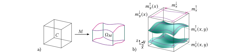
Its height functions do not intersect

and confine $\Omega_{M}$ along the three coordinate axes as shown in Figure 3. First, the constant height functions $m_{x}^{\uparrow}$ and, $m_{x}^{\downarrow}$ confine $\Omega_{M}$ along the $x$-axis. Second, the univariate height functions $m_{y}^{\downarrow}(x)$ and $m_{y}^{\uparrow}(x)$ confine $\Omega_{M}$ along the $y$-axis and, third, the bivariate height functions $m_{z}^{\uparrow}(x,y)$ and $m_{z}^{\downarrow}(x,y)$ confine $\Omega_{M}$ along the $z$-axis.

Inheriting the nested mappings’s properties, the Jacobian matrix $DM$,

is structured recursively. Its entries, $M_{xy},M_{xz},M_{yz}$,

require the first partial derivatives of the height functions. However, to evaluate the Jacobian determinant $J_{M}$,

partial derivatives are not required.

To increase the possible shapes of $\Omega_{M}$, the mapping can be oriented differently by rearranging $M$,

with a permutation matrix $Q$. By rearranging, $\Omega_{M}$ can be confined along the $x$-axis by a bivariate surface for example. Naturally, the mapping can be restricted to two-dimensional sets by dropping component $z$.

Our approach to construct a mapping, $A:C\rightarrow\Omega_{\alpha}$, is to match the codomain of a nested mapping to $\Omega_{\alpha}$. To match $\Omega_{\alpha}$, we disassemble its surface $\Gamma_{\alpha}$ into a set of height functions. This is possible if $\Gamma_{\alpha}$ and the intersections of $\Gamma_{\alpha}$ with suitable faces, edges and corners of the enclosing hyperrectangle $K$, are graphs on their associated coordinate planes.

To illustrate, let $\Omega_{\alpha}$ be a subset of the cube $K^{3}=[-1,1]^{3}$, such that its surface is a graph,

on its orthogonal projection $\Pi_{z}(\Gamma_{\alpha})$ onto the $xy$-plane (see figure 4). Hence, by embedding $a^{\uparrow}_{z}(x,y)$ in $K^{3}$, the graph’s function determines the first height function of the nested mapping. Forming the graph’s domain, the orthogonal projection flattens direction $h\in\{x,y,z\}$,

The projection utilizes height vector $\boldsymbol{e}_{h}$ which is $1$ at component $h$ and $0$ otherwise.

Further, let the intersection of the surface and the cube’s lower face $K^{2}$ be a graph on the orthogonal projection of the intersection onto the $xz$-plane,

Repeating the approach, the graph’s function $\gamma$ subsequently specifies the second height function of the nested mapping, $a^{\downarrow}_{y}(x)$.

Finally, the graph of the intersection of the cube’s edge $K^{1}$ and $\Gamma_{\alpha}$ on its projection onto the $yz$-plane,

determines the height function $a^{\uparrow}_{x}$.

When combined, the height functions define the nested mapping,

where each axis is respectively confined by a height function and a face, edge or point of $K^{3}$.

Algorithm 1 recursively creates a nested body $G=(K_{G},H)$ consisting of hyperrectangles. Beginning with a nested body consisting of a single level containing hyperrectangle $K$, it gradually deepens $G$ by selecting suitable height directions. Corresponding to the selected height direction, the algorithm adds a new level of hyperrectangles to $G$ while upholding the invariant: For each $k\in K_{G}$ with associated height direction $h\in H$, $\Gamma_{\alpha}\cap k$ is a graph on $\Pi_{h}(\Gamma_{\alpha}\cap k)$.

In each recursion, Algorithm 1 constructs a set of hyperrectangles $P$. After gathering the lowest level of hyperrectangles of $G$ in $P$, it removes each hyperrectangle $k$ from $P$ satisfying one of two conditions: First, if the hyperrectangle does not intersect $\Gamma_{\alpha}$, $\Gamma_{\alpha}\cap k=\emptyset$. Second, if the entire hyperrectangle is a subset of $\Gamma_{\alpha}$, $\Gamma_{\alpha}\cap k=k$. It removes them because the invariant holds unrestrictedly for these hyperrectangles and all contained faces, regardless of height direction. For all remaining hyperrectangles $k\in P$, Algorithm 1 chooses a common height direction $h$ and checks if the invariant holds. If it cannot be guaranteed, Algorithm 1 subdivides $G$ and restarts or designates $G$ for a brute force method. If the invariant can be guaranteed, it attaches the faces of $P$ as a new level of hyperrectangles to $G$.

Each new level of $G$ consists of the lower faces and the upper faces $F$ in direction $h$ of the hyperrectangles $P$,

The lower face, $\text{face}_{h}^{\downarrow}(k)$, and upper face, $\text{face}_{h}^{\uparrow}(k)$, of a hyperrectangle $k\in\mathbb{K}^{i},i>0,$

are subsets of the hyperrectangle’s boundary.

As long as $P$ contains hyperrectangles new levels are attached to $G$ until its deepest level consists of points. When Algorithm 1 has terminated, $\Gamma_{\alpha}$ is a graph whose domain is either a hyperrectangle or a subset of a hyperrectangle bounded by graphs. If the domain is bounded by graphs, their domains are in turn either hyperrectangles or subsets of hyperrectangles bounded by graphs, and so on. Illustrating the involved hyperrectangles, Figure 5 provides an example of a nested body created by Algorithm 1 for a planar $\Gamma_{\alpha}$.

So far, we have ommitted the inner workings of the algorithm’s components which we will discuss in the following. To decide if a hyperrectangle should be removed from $P$, we assess if $\Gamma_{\alpha}\cap k=\emptyset$ or $\Gamma_{\alpha}\cap k=k$ on the hyperrectangle $k$. This is equivalent to evaluating the sign $\in\{-,0,+,\pm\}$ of the level set on $k$,

The sign,

indicates if $\alpha$ can be uniformly bounded on a set $k$, not necessarily a hyperrectangle.

To evaluate the sign numerically, we approximate $\alpha(k)$ with a Bézier patch of degree $n$,

with $m=(n+1)^{\dim(k)}$ control points $q_{i}$ and basis functions $b_{i}$. The basis functions are Bernstein polynomials, tensorized to match the dimension of $k$. The control points are chosen so that $p$ interpolates $\alpha$ at equidistant data points, spanning a mesh including the boundary of $k$. Since the Bézier patch lies in their convex hull, the control points bound $p(k)$,

Utilizing the bound, we estimate the sign of $k$,

with a precision threshold $\epsilon$, necessitated by the limited precision of machine numbers. Relying on the convex hull of the approximation, the estimate may wrongly assess the body’s sign to be undetermined, $\pm$, in some cases. Fortunately, this only causes the algorithm to add unnecessary faces to $G$ without compromising the invariant. In rare cases, the estimate may wrongly determine a sign $\in\{-,0,+\}$ if $\alpha$ lies outside the convex hull of $p$ which could compromise correctness. However, practice has shown that $n=3$ suffices to reliably assign a sign to a body in a sufficiently resolved numerical grid.

As a way to determine a suitable height direction $h$ for the set of hyperrectangles $P$,

the index of the greatest entry of $\boldsymbol{y}$ is selected. The vector $\boldsymbol{y}$ denotes the average of the projections of each gradient $\nabla_{k}\alpha$ onto each hyperrectangle $k\in P$. Each projected gradient is evaluated at the center $\boldsymbol{c}_{k}$ of its associated hyperrectangle.

To decide if $\Gamma_{\alpha}\cap k$ is a graph over $\Pi_{h}(\Gamma_{\alpha}\cap k)$, we bound the gradient $\partial_{h}\alpha$ of the level set. It is a graph, if the component $h$ of $\partial_{h}\alpha$ does not change its sign on a hyperrectangle $k$,

Once again, we interpolate $\partial_{h}\alpha$ with a Bézier patch to evaluate its sign. Offering a conservative approximation, this estimate may deem surfaces, which are representable as graphs, unrepresentable and lead to unneeded subdivisions. However, it does not incorrectly evaluate the surface as representable as a graph which would contradict the invariant.

Finally, if $\Gamma_{\alpha}\cap k$ is not a graph over $\Pi_{h}(\Gamma_{\alpha}\cap k)$, the algorithm either subdivides $K$ and restarts or employs a brute force method, depending on the number of previous subdivisions. Since a linear polynomial is always a graph over the faces of a hyperrectangle, approximating $\alpha$ by a linear polynomial represents a convenient brute force method. If combined with a sufficiently large number of subdivisions, high accuracy can be maintained.

Algorithm 2 tesselates the root body $R$ of a nested body $G$ created by Algorithm 1,

so that each tile $v\in V$ is the codomain of a nested mapping and is either a subset of $R\cap\Omega_{\alpha}$ or $R\setminus\Omega_{\alpha}$. In order to create $V$, Algorithm 2 recursively splits $R$ into suitable subsets which are structured in nested bodies. Importantly, the subset $V^{-}$ of $V$,

is directly required for numerical integration since it tesselates the domain of the integral $R\cap\Omega_{\alpha}$.

When Algorithm 2 is called for the first time, it receives a nested body $G$ created by Algorithm 1 as input, $W=G$. In each subsequent iteration, Algorithm 2 processes the nested body $W$. It traverses the bodies of $W$ with undetermined sign, $\pm$, in reverse level order starting from the second deepest level, assigning a sign $\in\{-,0,+\}$ to each. Visiting each undetermined body $w$ of a level before moving upwards, it derives the sign of $w$ from the signs of its children, splitting $W$ when required. When finally the root has been assigned a sign, it is the codomain of a nested mapping.

The sign of an undetermined body $w\in K_{W}$ with height direction $h$ and children $w^{\downarrow}$ and $w^{\uparrow}$,

can be determined from the signs of its children if it fullfills three conditions. First, both children have a determined sign,

Second, $\Gamma_{\alpha}\cap w$ is a graph over $\Pi_{h}(\Gamma_{\alpha}\cap w)$. Third, the projections in height direction $h$ of $w$ and its two children $w^{\downarrow}$ and $w^{\uparrow}$ coincide,

If the three conditions hold, there are three different cases specifying $w$’s sign: First, if the body’s children $w^{\downarrow}$ and $w^{\uparrow}$ have the same sign $s\in\{-,+\}$, then $\Gamma_{\alpha}\cap w=\emptyset$ and $\text{sign}_{\alpha}(w)=s$. Second, if $w^{\downarrow}$ has a sign $s\in\{-,+\}$ and $w^{\uparrow}$ has sign $0$, then $\Gamma_{\alpha}\cap w=w^{\uparrow}$ and $\text{sign}_{\alpha}(w)=s$, or vice versa. Third, if $w^{\downarrow}$ and $w^{\uparrow}$ have a different sign $\in\{-,+\}$, then $\Gamma_{\alpha}\cap w$ lies between the children and the sign of $w$ stays undertermined, $\text{sign}_{\alpha}(w)=\pm$.

To assign a sign in the third case, the algorithm splits $W$ into two nested bodies, $W\rightarrow W^{\prime},\,W^{\prime\prime}$. It divides $w$ along $\Gamma_{\alpha}$ into two bodies, $w={w}^{\prime}\dot{\cup}{w}^{\prime\prime}$, and inserts a new child $w^{0}=\Gamma_{\alpha}\cap w$ with $\text{sign}_{\alpha}(w^{0})=0$,

The body-children triple of $w$ is split in two,

so that the projections of the new triples align (see Figure 6). After the split, the second case applies to the new bodies ${w}^{\prime}$ and ${w}^{\prime\prime}$. Hence, $\text{sign}_{\alpha}({w}^{\prime})=\text{sign}_{\alpha}(w^{\downarrow})$ and $\text{sign}_{\alpha}({w}^{\prime\prime})=\text{sign}_{\alpha}(w^{\uparrow})$.

In order to split $W$, not only $w$ has to be divided. To create the other bodies of $W^{\prime}$ and $W^{\prime\prime}$, the nodes that are part of a level higher than $w$’s are copied and added to $W^{\prime}$ and $W^{\prime\prime}$ in a first step. In a second step, every remaining node $v$ of $K_{W}$ is split, $v=v^{\prime}\dot{\cup}v^{\prime\prime}$, and inserted into the respective nested body. Each $v$ is split so that the projections in height direction $h$ of $v$,

of $v^{\prime}$ and its children $v^{\prime\uparrow}$ and $v^{\prime\downarrow}$, and $v^{\prime\prime}$ and its children $v^{\prime\prime\uparrow}$ and $v^{\prime\prime\downarrow}$ align. In particular, this means that each node $v$ of the level of $w$ receives a new child $v^{0}$ mirroring $w^{0}$,

as illustrated by Figure 6.

As long as an undetermined body is assigned a sign in each recursion and the three conditions are met by every body-children triple of $W$, the algorithm will terminate correctly. The three conditions are true when Algorithm 2 is called for the first time because they hold for each nested body created by Algorithm 1. Consequently, all three conditions remain true while the algorithm is iterating and $W$ is not split. When $W$ is split, it is easy to see that the second and the third condition are true for every body-children triple of $W^{\prime}$ and $W^{\prime\prime}$; The second condition holds because the bodies of $W^{\prime}$ and $W^{\prime\prime}$ are subsets of the bodies of $W$, and the third condition is enforced by construction. However, the first condition must be actively maintained by the algorithm.

To assert the first condition, each inserted body $v^{0}$ is assigned a sign after the split. In order to determine the sign, it suffices to evaluate $\alpha$ at any point $\boldsymbol{x}\in v^{0}$. This is the only time when explicitly computing a point on the body is required. To compute such a point, height functions are used.

Each nested body $W$ has $d$ pairs of height functions,

Initially, each height function is constant,

and correlates to a face of the hyperrectangle $R$ in the root of $W$. When a body $w$ of $W$ is split, the height functions $a_{j}^{\downarrow}=a^{\downarrow},a_{j}^{\uparrow}=a^{\uparrow}$ of $w$’s level are adjusted to match the shape of $W^{\prime}$ and $W^{\prime\prime}$ by inserting $a^{0}:\mathbb{R}^{d}\rightarrow\mathbb{R}$,

The inserted height function $a^{0}(\boldsymbol{x})$ describes the surface $\Gamma_{\alpha}\cap w$,

defined by the zero-isocontour of $\alpha$. To evaluate the implicit function, the Newton method,

References

- [1] Hong, Q., Wang, F., Wu, S., Xu, J., 2019. A unified study of continuous and discontinuous Galerkin methods. Sci. China Math. 62, 1-32. https://doi.org/10.1007/s11425-017-9341-1
- [2] Nguyen, V.P., Anitescu, C., Bordas, S.P.A., Rabczuk, T., 2015. Isogeometric analysis: An overview and computer implementation aspects. Mathematics and Computers in Simulation 117, 89-116. https://doi.org/10.1016/j.matcom.2015.05.008
- [3] Gottlieb, D., Turkel, E., 1983. Spectral methods for time dependent partial differential equations. Numerical Methods in Fluid Dynamics 1127.
- [4] Olsson, E., Kreiss, G., 2005. A conservative level set method for two phase flow. Journal of Computational Physics 210, 225-246. https://doi.org/10.1016/j.jcp.2005.04.007
- [5] Osher, S., Fedkiw, R.P., 2001. Level Set Methods: An Overview and Some Recent Results. Journal of Computational Physics 169, 463-502. https://doi.org/10.1006/jcph.2000.6636
- [6] Annavarapu, C., Hautefeuille, M., Dolbow, J.E., 2012. A robust Nitsche’s formulation for interface problems. Computer Methods in Applied Mechanics and Engineering 225-228, 44-54. https://doi.org/10.1016/j.cma.2012.03.008
- [7] Kummer F. Extended discontinuous Galerkin methods for two-phase flows: the spatial discretization. International Journal for Numerical Methods in Engineering. 2017;109(2):259-289. doi:https://doi.org/10.1002/nme.5288
- [8] Groß, S., Reusken, A., 2007. An extended pressure finite element space for two-phase incompressible flows with surface tension. Journal of Computational Physics, Special Issue Dedicated to Professor Piet Wesseling on the occasion of his retirement from Delft University of Technology 224, 40-58. https://doi.org/10.1016/j.jcp.2006.12.021
- [9] Wang, Y., Oberlack, M., 2011. A thermodynamic model of multiphase flows with moving interfaces and contact line. Continuum Mech. Thermodyn. 23, 409. https://doi.org/10.1007/s00161-011-0186-9
- [10] Wen, X., 2010. High Order Numerical Methods to Three Dimensional Delta Function Integrals in Level Set Methods. SIAM J. Sci. Comput. 32, 1288-1309. https://doi.org/10.1137/090758295
- [11] Wen, X., 2009. High order numerical methods to two dimensional delta function integrals in level set methods. Journal of Computational Physics 228, 4273-4290. https://doi.org/10.1016/j.jcp.2009.03.004
- [12] Wen, X., 2008. High Order Numerical Quadratures to One Dimensional Delta Function Integrals. SIAM J. Sci. Comput. 30, 1825-1846. https://doi.org/10.1137/070682939
- [13] Drescher, L., Heumann, H., Schmidt, K., 2017. A High Order Method for the Approximation of Integrals Over Implicitly Defined Hypersurfaces. SIAM J. Numer. Anal. 55, 2592-2615. https://doi.org/10.1137/16M1102227
- [14] Lehrenfeld, C., 2016. High order unfitted finite element methods on level set domains using isoparametric mappings. Computer Methods in Applied Mechanics and Engineering 300, 716-733. https://doi.org/10.1016/j.cma.2015.12.005
- [15] Bochkov, D., Gibou, F., 2019. Solving Poisson-type equations with Robin boundary conditions on piecewise smooth interfaces. Journal of Computational Physics 376, 1156-1198. https://doi.org/10.1016/j.jcp.2018.10.020
- [16] Cheng, K.W., Fries, T.-P., 2010. Higher-order XFEM for curved strong and weak discontinuities. International Journal for Numerical Methods in Engineering 82, 564-590. https://doi.org/10.1002/nme.2768
- [17] Fries, T.-P., Omerović, S., 2016. Higher-order accurate integration of implicit geometries. International Journal for Numerical Methods in Engineering 106, 323-371. https://doi.org/10.1002/nme.5121
- [18] Fries, T.P., Omerović, S., Schöllhammer, D., Steidl, J., 2017. Higher-order meshing of implicit geometries-Part I: Integration and interpolation in cut elements. Computer Methods in Applied Mechanics and Engineering 313, 759-784. https://doi.org/10.1016/j.cma.2016.10.019
- [19] Pan, S., Hu, X., Adams, N.A., 2018. A Consistent Analytical Formulation for Volume Estimation of Geometries Enclosed by Implicitly Defined Surfaces. SIAM J. Sci. Comput. 40, A1523-A1543. https://doi.org/10.1137/17M1126370
- [20] Engvall, L., Evans, J.A., 2017. Isogeometric unstructured tetrahedral and mixed-element Bernstein-Bézier discretizations. Computer Methods in Applied Mechanics and Engineering 319, 83-123. https://doi.org/10.1016/j.cma.2017.02.017
- [21] Antolin, P., Wei, X., Buffa, A., 2022. Robust numerical integration on curved polyhedra based on folded decompositions. Computer Methods in Applied Mechanics and Engineering 395, 114948. https://doi.org/10.1016/j.cma.2022.114948
- [22] Gunderman, D., Weiss, K., Evans, J.A., 2021b. Spectral Mesh-Free Quadrature for Planar Regions Bounded by Rational Parametric Curves. Computer-Aided Design 130, 102944. https://doi.org/10.1016/j.cad.2020.102944
- [23] Gunderman, D., Weiss, K., Evans, J.A., 2021a. High-accuracy mesh-free quadrature for trimmed parametric surfaces and volumes. Computer-Aided Design 141, 103093. https://doi.org/10.1016/j.cad.2021.103093
- [24] Müller, B., Kummer, F., Oberlack, M., 2013. Highly accurate surface and volume integration on implicit domains by means of moment-fitting. International Journal for Numerical Methods in Engineering 96, 512-528. https://doi.org/10.1002/nme.4569
- [25] Schwartz, P., Percelay, J., Ligocki, T., Johansen, H., Graves, D., Devendran, D., Colella, P., Ateljevich, E., 2015. High-accuracy embedded boundary grid generation using the divergence theorem. Communications in Applied Mathematics and Computational Science 10, 83-96. https://doi.org/10.2140/camcos.2015.10.83
- [26] Sommariva, A., Vianello, M., 2009. Gauss-Green cubature and moment computation over arbitrary geometries. Journal of Computational and Applied Mathematics 231, 886-896. https://doi.org/10.1016/j.cam.2009.05.014
- [27] Bui, H.-G., Schillinger, D., Meschke, G., 2020. Efficient cut-cell quadrature based on moment fitting for materially nonlinear analysis. Computer Methods in Applied Mechanics and Engineering 366, 113050. https://doi.org/10.1016/j.cma.2020.113050
- [28] Hubrich, S., Düster, A., 2019. Numerical integration for nonlinear problems of the finite cell method using an adaptive scheme based on moment fitting. Computers & Mathematics with Applications 77, 1983-1997. https://doi.org/10.1016/j.camwa.2018.11.030
- [29] Saye RI. High-Order Quadrature Methods for Implicitly Defined Surfaces and Volumes in Hyperrectangles. SIAM J Sci Comput. 2015;37(2):A993-A1019. doi:10.1137/140966290
- [30] Cui, T., Leng, W., Liu, H., Zhang, L., Zheng, W., 2020. High-order Numerical Quadratures in a Tetrahedron with an Implicitly Defined Curved Interface. ACM Trans. Math. Softw. 46, 3:1-3:18. https://doi.org/10.1145/3372144
- [31] Saye, R.I., 2022. High-order quadrature on multi-component domains implicitly defined by multivariate polynomials. Journal of Computational Physics 448, 110720. https://doi.org/10.1016/j.jcp.2021.110720
- [32] Beck L., F. Kummer, 2023. IntersectingQuadrature, GitHub repository. https://github.com/RumBecken/IntersectingQuadrature
- [33] Shampine LF. Vectorized adaptive quadrature in MATLAB. Journal of Computational and Applied Mathematics. 2008;211(2):131-140. doi:10.1016/j.cam.2006.11.021
- [34] Gonnet P. A review of error estimation in adaptive quadrature. ACM Comput Surv. 2012;44(4):22:1-22:36. doi:10.1145/2333112.2333117
- [35] Beck L., F. Kummer, 2023. Data of Numerical Experiments, TU datalib item. https://doi.org/10.48328/tudatalib-1175
Appendix A Hessian
The hessian of the composition ,