Competition-exclusion and coexistence in a two-strain SIS epidemic model in patchy environments
Abstract
This work examines the dynamics of solutions of a two-strain SIS epidemic model in patchy environments. The basic reproduction number is introduced, and sufficient conditions are provided to guarantee the global stability of the disease-free equilibrium (DFE). In particular, the DFE is globally stable when either: (i) , where is the total number of patches, or (ii) and the dispersal rate of the susceptible population is large. Moreover, the questions of competition-exclusion and coexistence of the strains are investigated when the single-strain reproduction numbers are greater than one. In this direction, under some appropriate hypotheses, it is shown that the strain whose basic reproduction number and local reproduction function are the largest always drives the other strain to extinction in the long run. Furthermore, the asymptotic dynamics of the solutions are presented when either both strain’s local reproduction functions are spatially homogeneous or the population dispersal rate is uniform. In the latter case, the invasion numbers are introduced and the existence of coexistence endemic equilibrium (EE) is proved when these invasion numbers are greater than one. Numerical simulations are provided to complement the theoretical results.
Keywords: Patch model; Epidemic model; Asymptotic Behavior; Competition-Exclusion; Coexistence.
2020 Mathematics Subject Classification: 34D05, 34D23, 91D25, 92D30, 37N25
1 Introduction
The novel human coronavirus disease 2019 (COVID-19) was first reported in the last trimester of 2019, and quickly spread around the world. The emergence of different strains of the disease generated significant concerns due to attendant waves after waves of infected populations across the world. As of March, 2020, the World Health Organization’s International Health Regulation Emergency Committee has declared the COVID-19 outbreak a Public Health Emergency of International Concern. In fact, in general, the questions of developing and implementing effective and adequate control strategies to alleviate the effects of infectious diseases, such as the COVID-19, on populations remain major concerns for public and health officials. These challenges are related in part to the lack of resources and good understanding of the dynamics of the disease. They are also significantly influenced by the unprecedented increase in human migration rates, which has made the word more interconnected. Hence, the studies of mathematical models, which incorporate population movements and environmental heterogeneity, may help public and health officials to take informed decisions and implement safe disease control strategies. In the current work, we study the large time behavior of solutions of a two-strain susceptible-infected-susceptible (SIS) epidemic model in patchy environments and investigate how the parameters of the model affect its dynamics. In particular, our results reveal the important of both spatial heterogeneity and population movements on the dynamics of infectious diseases.
Consider the Susceptible-Infected-Susceptible (SIS) two-strain epidemic model
| (1.1) |
where is the total number of individuals, is the number of patches, and . For and : is the total size of susceptible population on patch-; is the total number of infected population with strain- on patch-; and are positive numbers and stand respectively for the dispersal rates of susceptible population and infected population with strain-; is positive and represents the disease transmission rate resulting from interaction of the susceptible and infected population with strain- on patch ; is positive and represents the recovery rate from strain- on patch-. Note that the ’s terms do not appear in (1.1), so we set for convenience. For , is a nonnegative number and represents migration rate from the patch- to the patch-. Throughout this work, we shall suppose that the following standing assumption holds.
(A1) The matrix is nonnegative, symmetric and irreducible.
Assumption (A1) indicates that the migration rates between any two patches are the same and individuals can move directly or indirectly from any patch to another.
When the dispersal rates are neglected in (1.1), we obtain a particular type of a two-strain ODE-SIS epidemic model studied by Bremermann and Thieme in [8]. An important conclusion reached in [8] for (1.1) when is that the pathogen strain that does not optimize the basic reproduction number dies out asymptotically. This fact is known as the competition-exclusion principle in the literature. The basic reproduction number measures the expected number of secondary cases caused by a single index in an otherwise susceptible population. Since this interesting work, several studies have been devoted to investigate the competition-exclusion and coexistence of different strains of an infectious disease.
In [2], Ackleh and Allen examined the competition-exclusion and coexistence for pathogens in an SIR epidemic model with variable population size. In particular, under appropriate hypotheses on the parameters, they showed that several pathogens for a single host leads to exclusion of all pathogens except the one with the largest basic reproduction number. In [3], Acklesh and Allen extended their study to SIR and SIS epidemic models with multiple pathogen strains which assume total cross immunity, standard incidence, and density-dependent host mortality. Again, under some conditions on the parameters of these models, they established the competition-exclusion between multiple strains of the disease. For some related studies on multi-strain ODE models, we refer the interested readers to [5, 20, 7, 25, 26] and the references cited therein.
Assume that . Then system (1.1) reduces to a single-strain model, which was recently studied by Li and Peng [21]. In this setting, they introduced the single-strain basic reproduction number (see formula (2.9) below) and investigated the large-time behavior of solutions. Among other results, they established the global stability of the disease free equilibrium (DFE) if and either the local basic reproduction function (see formula (2.11) below) is constant or the population dispersal rate is uniform. However, when , they proved that the disease is endemic and the single-strain model has at least one endemic equilibrium (EE). Furthermore, the work [21] established the uniqueness of the single-strain EE under some additional assumptions, which include: (i) the dispersal rate of the susceptible group is greater or equal to that of the infected group, (ii) transmission rate is patch independent, and (iii) is constant. The asymptotic profiles of the single-strain EE as either the dispersal rate of the susceptible or infected groups approximate zero were also studied in [21]. The results of [21] extend some known results ([10, 14, 33, 35]) on the continuous diffusive models to the patch model.
Indeed, when dispersal movement of the population is assumed to occur locally and randomly in adjacent directions, the following PDE-SIS model
| (1.2) |
can be used to study the dynamics of the disease. In (1.2), is an open bounded domain in , , with a smooth boundary . denotes the outward normal unit derivative on . The parameters of (1.2) have the same meanings as those in the multiple patches model (1.1). Hence, the ODE-SIS system (1.1) can be seen as a discrete in space of the continuous in space PDE-SIS model (1.2). The two-strain PDE-SIS model (1.2) was first studied by Ackleh, Deng and Wu [4], then by Salako [29], and recently by Castellano and Salako [9]. In these works, the authors defined the basic reproduction number of (1.2) and studied the asymptotic profiles of coexistence steady states, and the large-time behavior of classical solutions. In particular, the authors of [4] established the competition-exclusion of the strains when the local reproduction functions are spatially homogeneous. In [29], sufficient criteria for existence and non-existence of coexistence EE equlibria of (1.2) are obtained. Moreover, the asymptotic profiles of coexistence EE solutions of (1.2) as the diffusion rates of some of the subgroups of the population converge to zero are established in [29]. The work [9] considered a more general model and also established the competition-exclusion of the strains if at least one strain local reproduction function is spatially homogeneous. Our results in the current manuscript examine the extent to which the findings of [4] and [9] on the PDE-SIS model hold for the two-strain multiple patches model (1.1). Furthermore, we establish some new results for the two-strain multiple patches model (1.1), which remain open for the PDE-SIS model 1.2. In particular, for system (1.1), Theorem 2.1 below establishes the uniform persistence of the susceptible population. It also establishes the global stability of the DFE when either the basic reproduction number is: (i) less or equal to the reciprocal of the total number of patches, or (ii) less than one and the dispersal rate of the susceptible population is sufficiently large.
The current work also examines the global dynamics of solutions of the two-strain SIS multiple patches system (1.1) and discusses the extent to which the competition-exclusion principle hold. In particular Theorems 2.2, 2.3, and 2.4 establish the competition exclusion of the strains under quite general assumption on the parameters of the model. Theorem 2.6 introduces the invasion numbers and establishes the coexistence of the strains when these numbers are greater than one.
There are several studies on the single-strain PDE-SIS epidemic model of system (1.2) (see [10, 14, 33, 35] and the references therein). Note that the force of infection used in the mathematical models (1.1) and (1.2) is , and refers as the mass-action or density-dependent transmission mechanism. Another popular transmission mechanism used in the modeling of infectious diseases is the standard or frequency-dependent infection mechanism, in which case the force of infection is given by . For some results on the single-strain epidemic models with the standard transmission mechanism, we refer to [1, 6, 13, 16, 17, 18, 22, 28, 27, 31, 36] and the references cited therein. See also [23, 24, 34] for some recent progress on the multi-strain diffusive epidemic model with standard transmission mechanism.
The rest of the paper is organized as follows. In section 2, we first introduce some notations and definitions, and then state our main results. We complete this section with some numerical simulations and some discussion of our main results. Section 3 introduces some preliminary results, essential for the clarity of our presentations. The proofs of our main results are given in section 4.
2 Notations, Definitions and Main Results
2.1 Notations and Definitions
For convenience, we introduce a few notations and definitions. First, we would like to rewrite system (1.1) is a compact form. To this end, let denote the square matrix with entries
| (2.1) |
It follows from assumption (A1) that the matrix is symmetric, irreducible and has nonnegative off diagonal entries. For each , let denote the column vector in , . Given two column vectors and in , define the Hadamard product , ,
and denote by the diagonal matrix with diagonal entries , . Using the above notations, system (1.1) can be written as
| (2.2) |
Due to biological interpretations of the vectors and , we will only be interested in nonnegative solutions of (2.2). Let denote the set of nonnegative real numbers. Note that the right-hand side of (2.2) is locally Lipschitz on . Hence, given an initial data , (2.2) has a unique solution defined on a maximal interval of existence . Observe that generates a strongly-positive matrix-semigroup on . We have endowed with the usual order induced by the cone of vectors with nonnegative entries . Hence, it follows from the comparison principle for cooperative systems that for every . A direct computation based on (1.1) gives
Hence,
| (2.3) |
from which we deduce that . Note also from (2.3) that solution operator of (2.2) is globally bounded. Thanks to (2.3) and the fact that the positive constant is fixed throughout the whole manuscript, the semiflow generated by solutions of (1.1) leaves invariant the set
It is easy to see that is a compact subset of , being closed and bounded. Note from (2.2) that if for some , for every , then for all and . However, since is irreducible with nonnegative off diagonal entries, if for some and , then for all and . We say that a solution has positive initial data if for each , for some .
A vector is an equilibrium solution of (2.2) if it satisfies the system of algebraic equation
| (2.4) |
Given a square matrix , we denote by its spectral bounds,
| (2.5) |
where is the real part of , and by its spectral radius,
where is the spectrum of .
A disease free equilibrium (DFE) is an equilibrium of the form . Since the matrix generates a strongly-positive semigroup and for each , then by the Perron-Frobenius theorem, . Moreover, is simple. For convenience, let denote the null vector in and denote the -column vector with entries ones, that is
It is easy to see that column vector is an eigenvector associated with . As a result, we obtain that is the unique DFE of (2.2). An equilibrium solution of (2.2) for which for every for some is called an endemic equilibrium (EE) solution of (2.2). An EE solution of the form (resp. ) is called a strain-1 (resp. strain-2) EE solution. An EE solution for which for each and is called a coexistence-EE solution.
Linearizing (2.2) at , we get
| (2.6) |
Note that for each , the second equation in (2.6) decouples from the first equation. Clearly, for each , the square matrix defined by
| (2.7) |
is invertible. Thanks to (2.6), for each , setting
| (2.8) |
and following the next generation matrix theory, strain-’s basic reproduction is given by
| (2.9) |
For each , it is well known that and have the same sign (see [1]). The basic reproduction of the two-strain model (2.2) is
| (2.10) |
For , it follows from [21] that (1.1) has a single-strain- EE solution if . The work [21] also provided sufficient conditions for the uniqueness and stability of single-strain EE of (1.1).
Given, and , the local basic reproduction on patch- of strain- is
| (2.11) |
and the two-strain local reproduction number is
| (2.12) |
Note that for each , where . We also introduce the following sets
The set represents the region of where strain-1 is able to spread more quickly than strain-2. Conversely, is the region of where strain-2 is more infectious than strain-1. The set is the region where strain-1 and strain-2 local reproduction functions are equal.
We complete this section by introducing the high/low-risk patches. Fix and . Patch- is said to be high-risk (resp. low-risk) patch for strain- if the local reproduction number is bigger (resp. smaller) than one on that patch, that is (resp. ). Hence the sets and given by
are called the strain-’s high-risk region and low-risk region, respectively. Note that in the absence of movement and when the other strain is absent, strain- is endemic on any patch in its high-risk region while it goes extinct on any patch in its low-risk region. Hence, thanks to the competition exclusion-principle, when , strain- is dominant and drives out strain- on any patch in . When and , Theorem 2.6 below establishes the existence of a coexistence EE solution of (1.1) for small diffusion rates of the population under some appropriate hypothesis.
2.2 Main Results
We state our main results. Our first result reads as follows.
Theorem 2.1.
- (i)
- (ii)
The DFE is linearly stable if and unstable if . Furthermore, the following conclusions hold.
- (ii-1)
If for some , then strain-l eventually dies out. In particular if , then the DFE is globally stable.
- (ii-2)
If for some , then there is such that the strain-l eventually dies out for any diffusion of susceptible population . In particular if , then there is such that the DFE is globally stable for any diffusion of susceptible population .
- (ii-3)
If for each , then the disease is persistence in the sense that there is a positive number such that for every solution with a positive initial data in ,
(2.14) Furthermore,
(2.15) where and .
- (ii-1)
Theorem 2.1-(i) indicates that the susceptible population persists uniformly, hence it will never be driven to extinction. On the other hand, thanks to Theorem 2.1-(ii-1), when , irrespective of the dispersal rate of the susceptible population, the disease will eventually go extinct. Recall that is independent of the dispersal rate of the susceptible population, and is the total number of patches. In the particular case of , the model reduces the single-patch ODE model for which it is well known that the DFE is globally stable if and only if So, our result is sharp in the case of single-patch model. Note also that, for large diffusion rate of the susceptible population, Theorem 2.1-(ii-2) shows that the DFE is globally stable when . When , that is there are at least two patches, the question of the global stability of the DFE remains open when and the dispersal rate of the susceptible is small. We expect that the answer to this question will dependent delicately on the details on the spatial distribution of the recovery and transmission rates and how the dispersal rates are selected. For example, when dispersal rates are uniform, Theorem 2.4 below shows that the DFE is globally stable whenever . Theorem 2.3 below also confirms that the same conclusion holds when the local reproduction functions are spatially homogeneous. In the case of the single-strain PDE-SIS model (1.2), Castellano and Salako [11] recently proved, under some appropriate hypotheses, the existence of at least two EE solutions when and is sufficiently small. We suspect that such result will also hold for the multiple patches SIS model (1.1).
When each strain’s basic reproduction number is bigger than one, Theorem 2.1-(ii-3) establishes the uniform persistence of the disease, but does not exclude the possibility of the extinction of one strain. Hence, it becomes pertinent to examine the conditions on the parameters of the model which lead to a competition-exclusion of the strains. This is carried out in Theorems 2.2, 2.3, and 2.4 below.
Our first result on the competition-exclusion of the strains when one local reproductive number is spatially homogeneous reads a follows.
Theorem 2.2.
Suppose that , , and is constant in .
- (i)
If , then the single strain- EE is linearly stable. Furthermore, if , then the single strain- EE is globally stable with respect to positive initial data.
- (ii)
If , then the single strain- is unstable. Furthermore, if , then for solutions of (1.1) with positive initial data, the strain- infected population eventually goes extinct while strain- persists uniformly in time.
Note that Theorem 2.2 can also be stated if we interchange the roles of strain-1 and strain-2. Now, suppose that strain-1 local reproduction function is spatially homogeneous, that is, its transmission and recovery rates are proportional to each other. If it also has the largest basic reproduction number, Theorem 2.2-(i) indicates that it cannot be invaded at equilibrium by an initially small size of the infected population with strain-2. If in addition, it strictly locally maximizes the local reproduction functions on all patches, then it drives the other strain to extinction. However, if strain-1 has a smaller basic reproduction number, Theorem 2.2-(ii) shows that it will be invaded at equilibrium by the other strain. Interestingly, these results hold irrespective of the dispersal rates of the population and suggest that the asymptotic dynamics of the solutions are independent of the dispersal rates when the local reproduction functions are spatially homogeneous. Our next result answers this question with an affirmation and provide a complete dynamics of solutions of (1.1) when both local reproduction functions are spatially homogeneous.
Theorem 2.3.
Suppose that is constant in for each .
- (i)
If , then the DFE is globally stable.
- (ii)
If , for . Then, the strain- EE solution is globally stable.
When the local reproduction functions are spatially homogeneous, Theorem 2.3 establishes that the strain with the largest basic reproduction number drives the other strain to extinction, irrespective of the dispersal rates of the population. In this case, the dispersal rates of the populations play no role on the asymptotic dynamics of solutions as it is determined by that of the model with no dispersal rate. To gain some understanding on how the dispersal rates may affect the global dynamics of the solutions of (1.1), in the next two results, we study the large time behaviors of solution in the special case of the following assumption.
(A2) .
Assumption (A2) means that the population dispersal rate is uniform and independent of the relevant subgroups of the population. In our next result, we again establish the competition-exclusion of the strains when at least one has its basic reproduction number less or equal to one.
Theorem 2.4.
Suppose that hypothesis (A2) holds. The following conclusions hold.
- (i)
If , then the DFE is globally stable.
- (ii)
If , , then the strain-l EE is globally stable with respect to positive initial data.
When hypothesis (A2) holds, that is the population’s dispersal rate is uniform and independent of the relevant subgroups, the basic reproduction numbers serve as threshold values for the global dynamics of solutions of (1.1). In this case, it follows from Theorem 2.4 that any strain whose basic reproduction number is less or equal to one eventually dies out. Note that, when both strain’s reproduction numbers are bigger than one, Theorems 2.2-2.3 provide sufficient conditions for the extinction of at least one strain. So, a natural question is to know whether both strains can coexist, and if so, provide some sufficient conditions on the parameters of the model which guarantee this. To tackle these questions, it seems appropriate to first introduce the strains’ invasion numbers, which measure the ability for a strain to invade another strain when rare.
Fix and suppose that . It follows from [21, Theorem 4] that (1.1) has at least one strain- EE solution. Under some further assumptions on the parameters of the model, [21, Theorem 4] established the uniqueness of the single-strain EE. When these assumptions do not hold, it is not clear whether single-strain EE are unique. Multiplicity of single-strain EE solutions for the PDE-SIS model (1.2) was recently established in [11]. So, for convenience, let
and denote the set of single-strain EE solutions of (1.1) in . It is clear that both and are compact sets and invariant under the semiflow of solutions of (1.1). Moreover, we have that and . Given and define
| (2.16) |
| (2.17) |
The quantity is the strain-l’s invasion number. Note that when (A2) holds, it follows from [21, Theorem 9] that consists of a single element for each . For any element and a subset , let
denote the distance from the point to the set . Our result on the coexistence EE of (1.1) reads as follows.
Theorem 2.5.
Suppose that . Let and be defined as in (2.17).
- (i)
If , then
(2.18) for every solution of (1.1) with initial data satisfying . Furthermore, if in addition is the global attractor for classical solutions of (1.1) with initial data in , then there is a positive number such that
(2.19) for every solution of (1.1) with initial data satisfying . Similar result holds for the strain-2.
- (ii)
Suppose that for each and hypothesis (A2) holds. Let be the uniform dispersal rate as in (A2). It follows from [21, Theorem 3] that (1.1) has a unique single-strain EE solutions and , where is the unique positive solution of the multiple-patch logistic equation
| (2.20) |
Furthermore, it holds that
| (2.21) |
As an application of Theorem 2.5, we can state the following result.
Theorem 2.6.
Suppose that hypothesis (A2) holds and . Let and denote the single-strain EE solutions of (1.1). Fix .
When hypothesis (A2) holds, and , Theorem 2.6 establishes the existence of a coexistence EE for small dispersal rate of the population. We expect that the same conclusion should hold when hypothesis (A2) is dropped. The questions of uniqueness and global stability of coexistence EE will be explored in our future work. Another interesting question is to investigate how the spatial distribution of the population at coexistence EE solutions depend on the dispersal rates. This question will also be investigated in our future work.
2.3 Numerical Simulations and Discussion
To further understand the dynamics of solutions of (1.1), we perform some simulations. Some of the simulations illustrate our theoretical results, while others explore some aspects that our theoretical results did not cover. For all the simulations, we consider two patches models, that is , and take and .
Simulation 2.3.1.
We fix the parameters: , , , , , , and . Next, we perform three simulations with three choices of the total population . (a) In Fig 1(a), we take , , and . Hence, , , , and . The simulations indicate an extinction of the disease. (b) In Fig 1(b), we take , , and . Hence, , , and . We also observe an exclusion of strain-2 while strain-1 persists. (c) In Fig1(c), we take , , and . Hence, , , and . In this case, we observe from Fig 1(c) that strain-1 persists while strain-2 eventually dies out. This agrees with persistence of at least one strain of the disease as predicted by Theorem 2.1-(ii-3). However, we notice an exclusion of strain-2 even though its basic reproduction number is bigger than one.


Simulation 2.3.2.
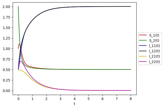
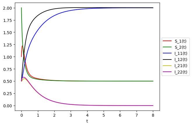
We fix the parameters: , , , and . So that is constant and . We also fix the initial data to , and . We then perform three simulations for different choices of the migration rates: (a) , and in Figure 2(a); (b) , and in Figure 2(b); and , and in Figure 2(c). We observe that strain-2 eventually dies out in all the three simulations irrespective of the choices of the migration rates. These agree with the conclusion of Theorem 2.2-(i).

Simulation 2.3.3.
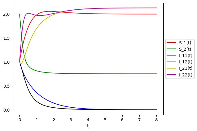
We fix the parameters: , , , and . So that is constant and . We also fix the initial data to , and . We then perform three simulations for different choices of the migration rates: (a) , and in Figure 3(a); (b) , and in Figure 3(b); and , and in Figure 3(c). We observe that strain-1 eventually dies out in all the three simulations irrespective of the choices of the migration rates. These agree with the conclusion of Theorem 2.2-(ii).


Simulation 2.3.4.
We fix the parameters: , , , and . So that is constant and . Next, we fix the diffusion rate of the infected population with strain-2. Finally, we fix the initial data to , and . We then perform three simulations for different choices of the migration rates and : and in Figure 4(a); and in Figure 4(b); and and in Figure 4(c). We notice that both strains coexist when the migration rates are small as illustrated by Figure 4(a), while strain-1 dies out for large diffusion rates as seen from Figures 4(b) and 4(c). These simulations complement Theorem 2.2 and suggest that the dynamics of the disease delicately depends on the choices of the migration rates when one of the strain local reproductive function is constant and neither maximizes nor minimizes the local reproductive functions.


Simulation 2.3.5.
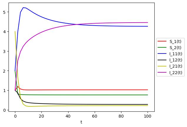
We fix the parameters: , , , and . So that is constant and . We also fix the initial data to , and , so that . Hence, and We then perform three simulations for different choices of equal migration rates : (a) in Figure 5(a); (b) in Figure 4(b); and in Figure 5(c). All the three simulations illustrate the coexistence of the strain. Hence, support the conclusions of Theorem 2.6. When the diffusion rates are sufficiently small, Fig 5(a) indicates a spatial segregation of the infected populations. However, for large diffusion rates, Figures 5(b) and 5(c) show that both strains persists uniformly on all patches.


2.3.6 Discussion
We examined the dynamics of solutions of a two-strain epidemic model in patchy environment. To this end, we introduced the basic reproduction number , and then first discussed the extinction of the disease under some sufficient conditions on the parameters of the models. In particular, Theorem 2.1 suggests that the disease would be eventually eradicated if either the basic reproduction number is smaller than the reciprocal of the total number of patches, or the migration rate of the susceptible population is sufficiently large and . However, at least one strain of the disease would persist if . Observing that the latter assertion does not exclude the possibility of extinction of at least one strain, we then investigated sufficient conditions which lead to the competition-exclusion principle. Simulations in Figure 1 provide an illustration of the dynamics of the disease as suggested by Theorem 2.1.
As noted in the introduction, in the celebrated work [8], Bremermann and Thieme showed that, when diffusion rates are neglected and there is only one patch, any strain that does not maximize the reproduction number would eventually die out. In Theorems 2.2 and 2.3, we showed that this conclusion extends to the multiple patches model with diffusion rates if the local reproduction function is patch independent. In fact, the conclusion of Theorem 2.2 is somehow stronger as it only requires that one strain to have its local reproductive function to be constant and to either maximize or minimize the local reproductive function on all patches. These results were perfectly illustrated by our simulations 2, 3, and 4. Interestingly, our simulations in Figure 4 indicate that the conclusions of Theorem 2.2 might not hold if some of the assumptions are dropped.
We further investigated some sufficient conditions on the parameters of the model which may lead to the coexistence of the strains. In this direction, we introduced the invasion numbers and then established the existence of coexistence EE when these numbers are bigger than one in Theorems 2.5 and 2.6. Our numerical simulations in Figure 5 support these theoretical results. An important question left open by our work is the uniqueness and global stability of the coexistence EE solution. Also, it would be interesting to study the effect of the diffusion rates on the spatial distributions of the coexistence EE as such information might help to developing and implementing adequate and effective disease control strategies. Another aspect that is not considered by our work is the effect of a total lockdown of one part of the population (say for example the movements of the infected populations are completely restricted) on the dynamics of the disease. We plan to devote some of our future studies on these open problems.
3 Preliminaries
We introduce some notations and collect a few preliminary results in the current section. For convenience, set
Note that for every . In general, given a column vector , set
Given and , we say that
and
Next, since is simple, and is real symmetric, there is an orthogonal matrix such that
where , are the eigenvalues of the symmetric matrix with . Hence,
| (3.1) |
Moreover, if we set , , as the column vectors of the square matrix , then is an orthonormal basis of . It then follows from (3.1) that
| (3.2) |
where denotes the inner product on . As a result, it follows from (3.2) and the fact that that
| (3.3) |
where . Note that so that
| (3.4) |
Observe also that
| (3.5) |
Let denote the standard orthonormal basis of . Recall that since is irreducible and cooperative, generates a strongly monotone semiflow on . Then
| (3.6) |
As a direct consequence of (3.6), we have the following Harnack’s inequality type, which plays an important in the proofs of our main results.
Lemma 3.1.
Let and such that
Let be a irreducible square matrix generating a strongly positive semigroup on . Then there is a positive number , such that any nonnegative solution of
| (3.7) |
satisfies
| (3.8) |
Proof.
Without loss of generality, we may suppose , otherwise we can replace by and by . Let be the positive eigenvalue of satisfying . Let be a nonnegative solution of (3.7). Then
This implies that
Hence
| (3.9) |
Next, for every , there is some such that
where is the standard orthonormal basis of . Observing that
then
In particular,
| (3.10) |
But, since is strictly positive, setting , for each , we have that
Therefore, in view of (3.10), we have that
which implies that
| (3.11) |
Finally, by (3.9) and (3.11), we have that
Therefore, (3.8) holds with . ∎
Remark 3.2.
Given a solution of (1.1) with initial data in , we have that
It then follows from Lemma 3.1 that there is a positive constant such that
| (3.12) |
Inequality (3.12) will be of significant to completing some of the proofs of our main results in the subsequent section. The following basic result on the uniform persistence of the susceptible population holds.
Lemma 3.3.
Let be a solution of (1.1) with initial data in . Then for all and
| (3.13) |
Proof.
Let be a solution of (1.1) with initial data in . We distinguish two cases.
Case 1. for every and . Then for every , and . This shows that satisfies
Hence, there is some such that . Hence for all .
The following results hold.
Lemma 3.4.
Fix and suppose that . There is such that
| (3.14) |
for any solution of (1.1) with a initial data in satisfying .
Proof.
First, note that since . We claim that (3.14) works with . Indeed, suppose by contradiction this is false. Hence, there is some initial data with such that
This in turn together with (2.2) imply that the function satisfies
| (3.15) |
where Let be a positive eigenvector associated with . Since , then there is some such that . It then follows from the monotonicity of the semiflow generated by the matrix semigroup and (3.15) that
which implies
As a result, . This contradicts with (2.3), so we deduce that the desired result hold. ∎
Lemma 3.5.
Fix and suppose that . Then there is such that
| (3.16) |
for every solution of (1.1) with an data in satisfying .
Proof.
Let be a solution of (1.1) with an initial data satisfying and set
Observe that
since is symmetric. Thus,
| (3.17) |
As a result, by the variation of constant formula,
4 Proofs of the Main Results
4.1 Proof of Theorem 2.1
We give a proof of Theorem 2.1.
Proof.
(i) Let be a solution of (1.1) with initial data in . Thanks to Lemma 3.3, we know that for all and that
Hence there is such that
Hence, for every , there is such that
But,
Therefore, in view of (4.1) and the monotonicity of , we have that
Therefore, setting for each and , then
which implies that (2.13) holds since by (3.6), and is independent of the initial data.
(ii) The fact that the DFE is linearly stable when and unstable when follows from standard results, (see for example [15, Theorem 2]). Next, we proceed to prove assertions (ii-1)-(ii-3).
(ii-1) First, suppose that for some . Hence, in view of (2.9), we have that
which is equivalent to
Now, let be a solution of (1.1) with initial data in . From (2.3) and (2.2), we have that
| (4.1) |
Hence, if denotes the positive eigenvector associated with with , it follows from (4.1) and the comparison principle that
As result, if , then as . Moreover, it follows from (3.19) and the fact that that
which yields the desired result.
Next, suppose that for some . For every , let be given by
Hence, since (4.1) holds, by the comparison principle, we deduce that is nonincreasing in . Thus
It is clear from the definition of that
| (4.2) |
We claim that
| (4.3) |
Indeed, since , it follows from the definition of that for each , there is such that
| (4.4) |
which implies that
Therefore, by (2.3),
This in turn implies that for all . Therefore,
Therefore,
This together with (4.4) implies that
which implies that . So (4.3) holds. Now, from (4.3) and (4.2) we have that as . Therefore, if , we can now proceed as in the previous case to establish that and as . This completes the proof of (ii-1).
(ii-2) Suppose that for some . Then . Therefore, by the continuity of the principal eigenvalue with respect to parameters, there is such that
Let denote the eigenvector of with and set
| (4.5) |
We now show that the desired result holds for any . So fix . Let be solution of (1.1) with a positive initial data in . Since for every , it follows from (3.19) that
Recalling that , then there is such that
This implies that
Hence, by the comparison principle,
In particular, if , taking , where is given by (4.5). We have that as for every . Moreover, we can proceed as in the proof of (ii-1) to prove that as for every .
(ii-3) Suppose that for each . We proceed in four steps.
Step 1. In the current step, we show that there is a positive constant such that
| (4.6) |
for any solution of (1.1) with a positive initial in . To see this, first recall that the set is compact, and invariant for the semiflow generated by classical solution of (1.1). Now define the mapping by
Clearly, the mapping is continuous. Furthermore, for every whenever and satisfies . Note from (3.16) that
Then applying persistence theory [30, Theorem 5.2], we deduce that (4.6) holds.
Step 2. In the current step, we show that there is a positive constant such that
| (4.7) |
for any solution of (1.1) with a positive initial. To this end, let be a solution of (1.1) with a positive initial data. Note that
which, thanks to the positivity of , implies that
Thus, setting , we obtain
| (4.8) |
Next, thanks to (4.6), there is such that
| (4.9) |
As a result,
Therefore, (3.2) holds for .
Step 3. Here, we show that
| (4.10) |
for any solution of (1.1) with a positive initial data. Let be a solution of (1.1) with a positive initial data. Thanks to (2.14), without loss of generality, we may suppose that
| (4.11) |
Observe from (2.2) that satisfies
where . Next set
Noting from (4.11) that
then
It then follows from the positivity of and the fact that that
from which we deduce that .
Step 4. Finally, we show that
| (4.12) |
for any solution of (1.1) with a positive initial data. We proceed as in step 3. This time we note that
where , and that the function
where is chosen such that , satisfies and
Thus, we deduce that for all , which implies that . This completes the proof of (iii). ∎
Thanks to the proof of Theorem 2.1-(iii), we can state the following result on the persistence of the disease for a single strain model.
Proposition 4.1.
Suppose that . Then there is a positive number such that for every solution with a initial data in satisfying and ,
| (4.13) |
Furthermore,
| (4.14) |
4.2 Proofs of Theorems 2.2 and 2.3
Lemma 4.2.
Suppose that for each , , and . Then, there exists such that
| (4.15) |
for every solution of (1.1) with initial data in satisfying .
Proof.
We proceed in two steps. First, note that . Since is constant in , and , then . So, we can choose such that . Let where and are given by (2.14) and 4.13, respectively. Set
Then
| (4.16) |
Step 1. We proceed by contradiction to establish that
| (4.17) |
for every solution of (1.1) with a positive initial data satisfying . So, suppose that there is a solution of (1.1) with a positive initial data satisfying and
| (4.18) |
Hence, after translation in time, we may suppose that
| (4.19) |
Observe that satisfies
| (4.20) |
where for each . Now, thanks to (2.14), (4.13) and (4.19), we have that and there is such that
Next, define
where is fixed and satisfies . Thanks to (4.16), we have
Hence, in view of (4.20), for all . Thus, satisfies
As a result, since , as , and , then as . This clearly, contradicts the fact that for all . Therefore, (4.17) must hold.
Step 2. We complete the proof of (4.15). Indeed, first recall that the set is compact, and invariant for the semiflow generated by classical solution of (1.1). Now define the mapping by
Clearly, the mapping is continuous. Furthermore, for every whenever and satisfies . Then applying persistence theory [30, Theorem 5.2], it follows from (4.17) that there is some such that
| (4.21) |
for every solution of (1.1) with a positive initial data satisfying . Finally, we can employ (3.12) to conclude that (4.15) follows from (4.21). ∎
Lemma 4.3.
Suppose that , for each and . Then, there exists such that
| (4.22) |
for every solution of (1.1) with initial data in satisfying .
Proof.
The proof follows a proper modification of that of Lemma 4.8, hence it is omitted. ∎
Lemma 4.4.
Suppose that and is constant in . Then the strain-1 EE is linearly stable if and unstable if .
Proof.
Set . Since is constant in , then and is the strain-1 EE solution. Linearizing (1.1) at this EE, we obtain the eigenvalue problem
| (4.23) |
in . Note that the third equation of (4.23) decouples from the first two equations. Let be an eigenpair of (4.23). If , then is an eigenvalue of the symmetric and irreducible matrix , hence it is a real number. If , then we have two cases. First, if , then is an eigenvalue of the symmetric and irreducible matrix , hence it is a real number. Next, if , then and is an eigenvalue of the symmetric and irreducible matrix , hence it is a real number. This shows that any eigenvalue of (4.23) is a real number. Now, we proceed in two cases to complete the proof of the lemma.
Case 1. Here, suppose that and show that is linearly stable. Since (see (2.9)), then , which is equivalent to This in turn implies that Observing that (since is constant in ), then
Therefore
| (4.24) |
Now, let be an eigenpair of (4.23). If , then, by (4.24), . If and , then either or . If , then
Finally, if , then and satisfies
Then is not strictly positive and is an eigenvalue of . It then follows from the Perron-Frobenius Theorem that . In view of the above, we see that any eigenvalue of (4.23) is negative, which implies that is linearly stable.
Case 2. Here, suppose that and show that is unstable. By the similar arguments leading to (4.24), we have that . Let be a positive eigenvector associated to . Since , then is in the resolvent set of . Thus, there is a unique solving the first equation of (4.23). Similarly, since , there is a unique solving the second equation of (4.23). Therefore, solves the first three equations of (4.23). Moreover, since is symmetric, we get
which yields that since . Therefore, solves (4.24) with . This shows that is unstable, since . ∎
Proof of Theorem 2.2.
Suppose that and is constant in .
(i) If , it follows from Lemma 4.4 that the strain-1 EE solution, , is is linearly stable. Next, suppose that . Let be solution of (1.1) with a positive initial data in . By Lemma 4.2, since , then there is such that
| (4.25) |
where is the positive number given in (4.15). Next, we claim that
| (4.26) |
Suppose by contradiction that (4.26) is false. Then there is a sequence of positive numbers converging to infinity such that
| (4.27) |
Since for all , by the Arzela-Ascoli theorem, there is a subsequence of and such that as , for on compact subsets of . Furthermore, satisfies
| (4.28) |
Moreover, thanks to (2.15) and (4.25),
| (4.29) |
Now, we claim that
| (4.30) |
To see this, observe from (4.28) and the fact that is symmetric that
since and (see (4.29)). Therefore,
| (4.31) | ||||
| (4.32) |
On the other, since
where we have used the fact that is symmetric, then
| (4.33) | ||||
| (4.34) |
From (4.31) and (4.33), we obtain that
Letting in this inequality yields (4.30). Therefore, (4.28) becomes
| (4.35) |
Setting , then by (4.29), , for every . Moreover, by (4.35) and the fact that , satisfies
which implies
for any . Hence for every , that is for every . As, a result, as , which contradicts with (4.27). Therefore, (4.26) holds. Therefore, for , there is such that for every . Hence,
which implies that as , since . Finally, by the similar computations yielding (3.17), we have that
where
It then follows from the variation of constant formula that
We can now employ (3.3) and (3.5), to derive that
Hence, letting and then in the right hand side of this inequality and recalling that (4.26), we obtain that
Therefore,
since as . This completes the proof of (i).
(ii) If , we know from Lemma 4.4 that is unstable. Now, suppose that (that is ) and we show that strain-1 eventually goes extinct. Let be solution of (1.1) with a positive initial in . We claim that
| (4.36) |
Suppose by contradiction that there is a sequence of positive numbers converging to infinity such that
Hence, by (3.12), there is such that
| (4.37) |
By the Arzela-Ascoli theorem, if possible after passing to a subsequence, there is such that as , for on compact subsets of . Furthermore, solves (4.28). By Lemma 4.3, there is such that
| (4.38) |
and by (2.15),
| (4.39) |
Moreover, by (4.37), we have that
| (4.40) |
From the second equation of (4.28) and the fact that is symmetric, we get
Integrating this equation yields
| (4.41) |
Thus, in view of (4.39), we obtain
| (4.42) |
and
| (4.43) |
From (4.40) and (4.42), we get
As a result, it follows from (3.12) that
We then conclude from (4.42) and the last inequality that
| (4.44) |
Next, from (4.28), we have that
| (4.45) | ||||
| (4.46) |
where we have used (4.39). An integration of the last inequality gives
This along with (4.38) and (4.44) yield
This is clearly impossible since . Therefore, (4.36) must hold. This together with (2.15) implies that for some positive number in dependent of initial data. This completes the proof of the theorem. ∎
Next, we give a proof of Theorem 2.3.
Proof of Theorem 2.3.
We suppose that is constant in for each . Hence for each . Fix . We distinguish three cases.
Case 1. . In this case, it follows from Theorem 2.2 that the strain-l EE is globally stable with respect to positive initial data.
Case 2. . Without loss of generality, we suppose that and . Let be solution of (1.1) with a positive initial data in and define
| (4.47) |
Clearly, for every and uniformly bounded above by . Moreover,
Therefore, is a Lyapunov function. It then follows from the LaSalle’s invariant principle ([19, Theorem 4.3.4]), the maximal invariant set, , of is the global attractor for solutions of (1.1). Now, observe that if and only if
| (4.48) |
As a result since and is invariant for the semiflow generated by solutions of (1.1) on , we conclude from (4.48) that it is a subset of the spatially homogeneous EE solutions. Thus which is equivalent to
Note here that (1.1) doesn’t have a strain-2 constant EE solution since . It is clear that and is invariant for the semiflow generated by solution of (1.1). Therefore, . However, since , the DFE solution is a repeller for solutions of (1.1) with positive initial data (see Lemma 3.4). Therefore, is the global attractor for solution of (1.1)
Case 3. . In this, consider again the Lyapunov function introduced in (4.47). This time we have that . Hence the DFE attracts all solutions of (1.1) with initial data in .
Observe that (i) of the theorem follows from case 3, while statement (ii) follows from case 1 and case 2. ∎
4.3 Proofs of Theorems 2.4, 2.5 and 2.6
Proof of Theorem 2.4.
Suppose that . Let be solution of (1.1) with a positive initial data in . Then
It then follows from (3.3) and (3.4) that
Therefore,
| (4.49) |
As a result,
| (4.50) |
Now, suppose that for some . This implies that . Let be the positive eigenvector associated with satisfying . Observe that
| (4.51) |
From (4.50) and (4.51), we obtain that
| (4.52) |
Since is symmetric, it then follows that
| (4.53) | ||||
| (4.54) | ||||
| (4.55) | ||||
| (4.56) |
Therefore, since , and hence as , we then conclude that as . Consequently, as since is strictly positive.
(i) Now, if , it follows from the above that as , for every . This together with (3.19), yields that as . This shows that the DFE is globally stable if . So, (i) is proved.
(ii) Suppose without lost of generality that . We know from the above that as , which implies that as . Recalling that satisfies (4.49) and (4.50). and
we can employ a perturbation argument to conclude that as , where is the unique positive solution of the multiple-patch logistic system
The existence of follows from standard results on the logistic equations and the fact that . Note that the last inequality holds since . We then conclude from (4.49) that as . This completes the proof of (ii). ∎
Proof of Theorem 2.5.
Suppose that , . Let and be defined by (2.17).
(i) Suppose that . Let such that . Take . Let be an eigenvector, with positive entries, associated with , that is satisfies
which is equivalent to
Hence, since is symmetric,
So, an integration of this yields that
from which it follows that
Since, for all , letting in the last inequality implies that (2.18) holds.
Next, suppose in addition that is the global attractor for classical solutions of (1.1) with initial data satisfying . We appeal to the persistence theory [30] to prove (2.19). To this end, define
| (4.57) |
Clearly, is continuous. Moreover, by the uniqueness of solution of (1.1), we see that for any given initial data , for some if and only if for all Since , by Lemma 3.4, we know that there is such that
| (4.58) |
Note also from (2.18) there there is such that
Therefore,
| (4.59) |
Now, we claim that there is a positive such that
| (4.60) |
We proceed by contradiction. So, suppose that there a sequence of initial data in satisfying and
| (4.61) |
By (2.14), there is , such that, for each , there is such that
| (4.62) |
It then follows from (4.61) that there is
| (4.63) |
However, thanks to (4.59), for each , there is , , as , such that
| (4.64) |
Finally, consider the sequence of solutions of (1.1). By the Arzela-Ascoli theorem, possibly after passing to a subsequence, there is a nonnegative solution of (1.1), defined for all , such that as , locally uniformly on . Clearly, by (4.61), for all . Moreover, we claim that
| (4.65) |
To see this, note from (4.63) and the fact that as that for all . This also implies that for all . Therefore, since is the global attractor for solutions of (1.1), when restricted to initial data , and (4.58) holds, it follows from [30, Theorem 5.7] that (4.65) holds. As a result, we obtain that , which contradicts with (4.64). Therefore, claim (4.60) holds. We can now invoke persistence theory [30, Theorem 5.2], we deduce that there is such that
Therefore, by the similar arguments as those in the proof of step 2 of Theorem 2.1-(ii-3) derive that (2.19) holds.
(ii) Suppose that desired hypotheses hold. Define the mapping by
Then is continuous and concave. Note that for all if . Furthermore, by (4.58), there is such that
Therefore, since the set is convex and compact, and the semiflow induced by the solutions of (1.1) is also compact and continuous, we can invoke [30, Theorem 6.2] to conclude that system (1.1) has at least one coexistence EE solution. ∎
We conclude this section with a proof of Theorem 2.6.
Proof of Theorem 2.6.
Suppose that (A2) holds and . Let and be the single-strain EE solutions of (1.1). It follows from [21, Theorem 3] that the single strain EE solution are globally stable with respect to positive initial on each of the set and . Hence, the assertions (i) and (ii) follows from Theorem 2.5.
(iii) By [12, Theorem 2.7], as , for each . Hence, since for each , , there is such that for every . This ensures that the unique single-strain EE solutions, and , exist whenever . Moreover, by [21, Theorem 9-b], it holds that
Therefore, by [12, Theorem 2.7], it holds that
| (4.66) |
However, for each and , it holds that and , that is, . Therefore, . Hence, by (4.66), there is such that for every . ∎
References
- [1] Allen, L. J. S., Bolker. B. M, Lou., Y., Nevai, A. L.: Asymptotic profiles of the steady states for an SIS epidemic patch model. SIAM J Appl Math., 67, 1283-1309 (2007).
- [2] Ackleh, A.S., Allen, L.J.S.: Competitive exclusion and coexistence for pathogens in an epidemic model with variable population size. J. Math. Biol. 47, 153-168 (2003).
- [3] Ackleh, A.S., Allen, L.J.S.: Competitive exclusion in sis and sir epidemic models with total cross immunity and density-dependent host mortality. Disc. Cont. Dyn. Sys. series B 5(2), 175–188 (2005).
- [4] Ackleh, A.S., Deng, K., Wu, Y.: Competitive exclusion and coexistence in a two-strain pathogen model with diffusion. Mathematical Biosciences and engineering 13(1), 1–18 (2016).
- [5] Allen, L.J.S., Langlais, M., Phillips, C. J.: The dynamics of two viral infections in a single host population with applications to hantavirus. Mathematical Biosciences 186(2), 191-217 (2003).
- [6] Allen, L.S.J., Bolker, B.M., Lou, Y., Nevai, A.L.: Asymptotic profiles of the steady states for an sis epidemic reaction-diffusion model. Disc. Cont. Dyn. Sys. 21(1), 1–20 (2008).
- [7] Bichara, D., Iggidr, A., Sallet, G.: Global analysis of multi-strains SIS, SIR and MSIR epidemic models. J. Appl. Math. Comput. 44, 273–292 (2014).
- [8] Bremermann, H.J., Thieme, H.R.: A competitive exclusion principle for pathogen virulence. J. Math. Biol. (1989).
- [9] Castellano, K., Salako, R.B.: Dynamics of classical solutions of a multi-strain diffusive epidemic model ( arXiv:2307.15155 ).
- [10] Castellano, K., Salako, R.B.: On the effect of lowering population’s movement to control the spread of an infectious disease. Journal of Differential Equations 316, 1–27 (2022).
- [11] Castellano, K., Salako, R.B.: Multiplicity of endemic equilibria for a diffusive SIS epidemic model with mass-action transmission mechanism, preprint.
- [12] Chen, S., Shi, J., Shuai, Z., Shuai, Z., Wu, Y.: Asymptotic profiles of the steady states for an SIS epidemic patch model with asymmetric connectivity matrix. J. Math. Biol. 80, 2327–2361 (2020).
- [13] Cui, R., Lam, K.Y., Lou, Y.: Dynamics and asymptotic profiles of steady states of an epidemic model in advective environments. J. Differential Equations 263(4), 2343–2373 (2017).
- [14] K. Deng, Y. Wu, Dynamics of a susceptible-infected-susceptible epidemic reaction-diffusion model, Proc. Roy. Soc. Edinburgh Sect. A, 146 (2016), 929-946.
- [15] P. V-D. Driessche, James Watmough, Reproduction numbers and sub-threshold endemic equilibria for compartmental models of disease transmission, Mathematical Biosciences, 180 (2002) 29–48.
- [16] Gao D.: Travel frequency and infectious disease. SIAM J. Appl. Math. 79, 1581-1606 (2019).
- [17] Gao, D.: How does dispersal affect the infection size? SIAM J. Appl. Math. 80(5), 2144-2169 (2020).
- [18] Gao, D., Lou, Y.: Impact of state-dependent dispersal on disease prevalence. J. of Nonlinear Sciences 31(17), 1-41 (2021).
- [19] D. Henry, Geometric Theory of Semilinear Parabolic Equations, Springer-Verlag Berlin Heidelberg, 1981.
- [20] Iannelli, M., Martcheva, M., Li, X-Z.: Strain replacement in an epidemic model with super-infection and perfect vaccination. Mathematical Biosciences, 195(1), 23-46 (2005).
- [21] Li, H., Peng, R.: An SIS epidemic model with mass action infection mechanism in a patchy environment. Studies in Applied Matehmatics, DOI: 10.1111/sapm.12553, 1-55 (2023).
- [22] Lou, Y., Salako, R. B., and Song, P.: Human Mobility and Disease Prevalence, Journal of Mathematical Biology, 87, no. 1, 1-32, (2023).
- [23] Lou, Y., Salako, R. B.: Control strategy for multi-strain epidemic model. Bulletin of Mathematical Biology, 84(10) 1-47 (2022).
- [24] Lou, Y., Salako, R. B.: Mathematical analysis of the dynamics of some reaction-diffusion models for infectious diseases. Journal of Differential Equations, 370, 424-469, (2023).
- [25] McCormack, R. K., Allen, L. J. S.: Multi-patch deterministic and stochastic models for wildlife diseases. Journal of Biological Dynamics, 1(1), 63–85 (2007).
- [26] Meehan, M. T., Cocks, D. G., Trauer, J. M., and McBryde, E. S.: Coupled, multi-strain epidemic models of mutating pathogens. Mathematical Biosciences, 296, 82-92 (2018).
- [27] Peng, R., Yi, F.: Asymptotic profile of the positive steady state for an SIS epidemic reaction-diffusion model: Effects of epidemic risk and population movement. Phys. D, 259, 8-25 (2013).
- [28] Peng, R.: Asymptotic profiles of the positive steady state for an sis epidemic reaction-diffusion model i. J. Differential Equations 247, 1096–1119 (2009).
- [29] Salako, R. B.: Impact of environmental heterogeneity, population size and movement on the persistence of a two-strain infectious disease, Journal of Mathematical Biology, 1-36 (2023).
- [30] Smith, H. L., Thieme, H.R.: Dynamical systems and population persistence. Graduate. Studies in Mathematics 218 (2011).
- [31] Song, P., Lou, Y., Xiao, Y.: A spatial seirs reaction-diffusion model in heterogeneous environment. J. Differential Equations 267, 5084–5114 (2018).
- [32] Van den Driessche, P., Watmough, J.: Reproduction numbers and sub-threshold endemic equilibria for compartmental models of disease transmission. Math. Biosci., 180, 29–48 (2002).
- [33] Wen, X., Ji, J., Li, B.: Asymptotic profiles of the endemic equilibrium to a diffusive SIS epidemic model with mass action infection mechanism. J. Math. Anal. Appl. 458, 715-729 (2018).
- [34] Wu, Y., Tuncer, N., Martcheva, M.: Coexistence and competitive-exclusion in sis model with standard incidence and diffusion. Disc. Cont. Dyn. Sys. series B 22(7), 1167–1187 (2017).
- [35] Wu, Y., Zou, Z.: Asymptotic profiles of steady states for a diffusive SIS epidemic model with mass action infection mechanism. J. Diff. Equat., 261, 4424–4447 (2016).
- [36] Yang, F-Y., Li, W-T., Ruan, S.: Dynamics of a nonlocal dispersal SIS epidemic model with Neumann boundary condition. J. Diff. Equ., 267(3), 2011-2051 (2019).