Homogenising SoHO/EIT and SDO/AIA 171Å Images: A Deep Learning Approach

The EIT-Sun-AIA angle, focal length and detector differences necessitate re-projecting EIT, AIA images to a common point-of-view and field-of-view. We use the ‘reproject’ module of Python to map AIA images to EIT detector with 4 times the original resolution of EIT (Figure 2). The re-projection of the corona is non-trivial. So, we make an assumption that coronal structures lie on a sphere centered on Earth, with a radius of Sun-Earth distance.

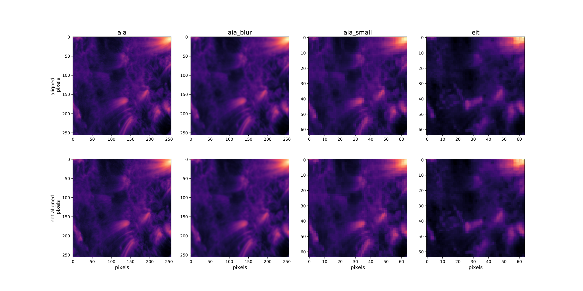
Re-projection is insufficient when we want to perform one-to-one mapping of EIT to AIA patches. Several other factors such as resolution, and optical aberration result in pixel shifts and may affect our homogenization objective. To make an accurate alignment we perform template matching (Brunelli 2009) using the following steps-

1. 1.

   Divide the EIT full disc images into contiguous non-overlapping $64\times 64$ patches.

2. 2.

   Blow up each of those patches by 4 times and map that location to the re-projected AIA.

3. 3.

   Correlate that blown-up EIT patch within the corresponding AIA location having a margin of (1/8)^th patch size on all 4 sides.

4. 4.

   Find the 256$\times$256 region from the AIA window providing the best correlation.

5. 5.

   Follow the above steps after generating another set of non-overlapping patches bounded by the center pixels of the original patches.

The steps above produce 365 patch-pairs [64$\times$64 EIT, 256$\times$256 AIA] per full-disc EIT-AIA image-pair (Figure 3).

We sample decade-long data (05/2010- 12/2020) within the training, validation, and test set by adding the first 7 months of each year to the training set, August and September to the validation set, and, the rest to the test set. We also put the entire 2015 data aside in the test set and tune the model hyperparameters based on the validation set performance.

We prepare the Deep learning (DL) model to transform 64$\times$64 EIT patches to 256$\times$256 AIA patches. The model is based on the super-resolution convolution neural net (CNN) presented in Deudon et al. 2020. However, our network is simple as we don’t have multiple views and avoid shift-net by pre-aligning the EIT, and AIA patches. The model consists of an encoder and a decoder structure. The encoder consists of 2D convolution layers and residual blocks. The decoder consists of 4x upsampling and 2D convolution layers. In each residual block, two convolution layers are used and the convolution layer outcome is added to the input layer to generate the output. We use a kernel size of $5\times 5$, 32 feature layers and a parametric ReLU activation in all the convolution layers except for the final layer that has only one feature layer and a kernel size of $1\times 1$. We use reflection padding the deal bring edge continuity in the adjacent super-resolved tiles.

To minimize the difference between the target ($T$) and DL predicted ($P$) image we consider the following as elements of loss function-

1. 1.

   Mean squared error: $MSE=\frac{1}{N}\sum_{i}{(T_{i}-P_{i})^{2}}$ where $N$ stands for the number pixels in output patches.

2. 2.

   Histogram (Wang et al. 2018) difference: $H=\frac{1}{K}\sum_{i}{(HT_{i}-HP_{i})^{2}}$ where $K$ stands for the number of bins in the histograms.

3. 3.

   Negative of Structural Similarity Index Metric (Zhou Wang et al. 2004): $S=-\frac{(2\mu_{T}\mu_{P}+C_{1})(2\sigma_{T,P}+C_{2})}{(\mu_{T}^{2}+\mu_{P}^{2}+C_{1})(\sigma_{T}^{2}+\sigma_{P}^{2}+C_{2})}$ with $C_{1}=(K_{1}L)^{2},C_{2}=(K_{2}L)^{2}$, $L$ being dynamic range and $K_{1},K_{2}\ll 1$. $\mu_{X},\sigma_{X},\sigma_{X,Y}$ respectively represent mean of $X$, standard deviation of $X$ and covariance of $X,Y$

4. 4.

   Gradient difference: $G=\frac{1}{N}\sum_{i}{(\nabla_{x}T_{i}-\nabla_{x}P_{i})^{2}}+\frac{1}{N}\sum_{i}{(\nabla_{y}T_{i}-\nabla_{y}P_{i})^{2}}$

Our objective is to perform the best performing weighted combination of $MSE$ and one of the other losses. To identify the weights we combine $MSE$ with each of the remaining components and calculate the best weight through a set of diagnostics as described in the following subsection.

Having a small amount of training data it is important that we estimate the uncertainty in model inference. We use a state-of-the-art technique called Approximately Bayesian Ensembling (ABE) that draws a set of anchor weights from a prior distribution and factor them through an additional regularization term to the loss function defined by-

where $diag(\mathbf{\Gamma})_{i}=\frac{\sigma_{\epsilon}^{2}}{\sigma_{prior,i}^{2}}$ and $N$ is the number of datapoints
During the training phase, the weights ($\boldsymbol{\theta}_{n}$) are optimized but the anchors ($\boldsymbol{\theta}_{anchor,n}$) are kept unchanged. We randomly select a set of four anchors and optimize a model for each giving rise to the ensemble of models. Here the index $n$ runs over the ensemble members. We set $\sigma_{\epsilon}^{2}$ to be the mean of the AIA patch histogram. We use anchored regularization in the last layer of our model to select both priors and anchors from a Glorot uniform (Glorot & Bengio 2010) distribution with $\sigma_{prior,i}^{2}=\frac{6}{n_{l}+n_{l+1}}$ where $n_{l}$ and $n_{l+1}$ are the numbers of units in two consecutive layers. We rewrite $diag(\mathbf{\Gamma})_{i}$ as $\frac{k_{1}(n_{l}+n_{l+1})}{6}$. We use $k_{1}$ (with a default value of $\sigma_{\epsilon}^{2}\approx 0.5$) to change the regularization weight and another parameter $k_{2}$ (with a default value of 1) to scale the standard deviation of the anchor weight distribution. We examine the sensitivity of the results to the anchored regularization with different values of $k_{1}$ (later referred to as ‘LAMBDA’) and $k_{2}$ (later referred to as ‘SD’).

We develop a set of diagnostics to compare the model inference between the baseline and outcomes for different loss function combinations. For this purpose, we collect all the validation patch pairs and model inference on those. We generate 2-dimensional histograms through logarithmic binning (uniform bins in log space) from the tuple of pixel intensity from model inference and target. We calculate the median and standard deviation for each inferred intensity bin. This generates a curve representing the expected AIA target and uncertainty for each inferred value. From those, we estimate the deviation from the expected rule i.e. ‘target = expected’. We name that metric as ‘% relative residual’. We also add a metric called ‘% relative variance’ representing the standard deviation and median ratio.

From the visual inspection and metrics (Figures 4,5), we find that all the DL outcomes give rise to superior results as compared to those corresponding to simple Upsampling and scaling. As depicted in Figure 4, the DL outcomes get rid of the bright point-like artifact present in the EIT patch. Among the DL outcomes, we use MSE loss as a baseline and examine the improvement caused by additional terms in the loss function. We find that unlike MSE additional loss terms drive the ‘% relative residual’ to be within $\pm 5\%$ for an inferred intensity range of [0,6] (Figure 5). We also observe that MSE + 400*Grad performs the best for higher intensities ($>6$). Also, by visual inspection, one can discern finer details in MSE+400*Grad more easily as compared to other DL outcomes.

The results show that (although better than the baseline) the deep-learning model cannot reach the same level of detail as the target AIA 171 Åimages (Figure 4). This could be because of the ill-posed nature of the problem with AIA having higher diffraction-limited resolution and better pixel pitch than EIT. It could also be the limited training data that is not able to constrain the outcome enough or that the small-scale information can’t be uniquely recovered from the large scale. More experiments should be performed to understand the optimal number of loss function terms beyond which performance can’t be improved given the size of the training data. Recent advancement in conditional GANs also inspires further experiments to bring back surface texture information but physical validation is needed for them to be fit for scientific applications.

We select four anchors and train a model with each of those without changing the training and validation set. Initially, we train the model with 20000 EIT-AIA patch pair and then increase the number of training patches to 70000. To record the change in performance, we generate 2-dimensional histograms between ensemble standard deviation vs. input EIT intensity over all the patch pixels for training, validation, and test sets. The ensemble standard deviation ($\sigma_{ensemble}$) is calculated over 64 pixels (4$\times$4 for 4 models) corresponding to each EIT pixel. From 2D histograms, we find a clear impact of training set size on the ensemble uncertainty. We observe that for each EIT intensity, the distribution of ensemble uncertainty when trained with 70000 patches shifts towards smaller values as compared to when trained with 20000 patches (Figure 6).

We also record changes in the distribution of ensemble standard deviation ($\sigma_{ensemble}$) for values of input intensity and parameters defining anchor distribution ($k_{2}$ or ‘SD’) and weightage of the regularization term ($k_{1}$ or ‘LAMBDA’) in the loss function over training, validation, and test set. It appears that for all the input intensities and anchor parameters, the $\sigma_{ensemble}$ distributions have a longer tail in the validation and test set as compared to the training set. The difference between validation/test and training set distribution diminishes for higher input intensities. However, the distributions get wider for higher input intensities. We don’t find as pronounced an effect by changing the anchor parameters. However, a close inspection reveals that the distribution gets wider with a reduction in regularization weightage for I=0.64. Also, for I = 0.76 the second peak in the distribution gets less pronounced for lower weightage (Figure 7).

On a representative solar image quadrant, we find that regions that are not well represented in the training data (e.g. coronal regions) produce high disagreement among the ensembles. Also, structures of non-solar origin generate high uncertainty (Figure 8).

It is unknown at this moment how many ensemble members are optimal beyond which the uncertainty in reconstruction converges. Further investigations are needed for that.

References

- Brunelli (2009) Brunelli, R. 2009, Template Matching Techniques in Computer Vision: Theory and Practice (Wiley Publishing)
- Chatterjee et al. (2022) Chatterjee, S., Muñoz-Jaramillo, A., & Lamb, D. A. 2022, Nature Astronomy, 6, 796
- Delaboudinière et al. (1995) Delaboudinière, J. P., et al. 1995, Sol. Phys., 162, 291
- Deudon et al. (2020) Deudon, M., et al. 2020, HighRes-net: Recursive Fusion for Multi-Frame Super-Resolution of Satellite Imagery
- Gal & Ghahramani (2015) Gal, Y., & Ghahramani, Z. 2015, arXiv e-prints, arXiv:1506.02142
- Glorot & Bengio (2010) Glorot, X., & Bengio, Y. 2010, in Proceedings of Machine Learning Research, Vol. 9, Proceedings of the Thirteenth International Conference on Artificial Intelligence and Statistics, ed. Y. W. Teh & M. Titterington (Chia Laguna Resort, Sardinia, Italy: PMLR), 249–256
- Jarolim (2022) Jarolim, R. 2022, in Proceedings of the 2nd Machine Learning in Heliophysics, 39
- Jungbluth et al. (2019) Jungbluth, A., et al. 2019, arXiv e-prints, arXiv:1911.01490
- Lemen et al. (2012) Lemen, J. R., et al. 2012, Sol. Phys., 275, 17
- Pearce et al. (2018) Pearce, T., Leibfried, F., Brintrup, A., Zaki, M., & Neely, A. 2018, arXiv e-prints, arXiv:1810.05546
- Wang et al. (2018) Wang, Z., Li, H., Ouyang, W., & Wang, X. 2018, CoRR, abs/1804.09398
- Zhou Wang et al. (2004) Zhou Wang, Bovik, A. C., Sheikh, H. R., & Simoncelli, E. P. 2004, IEEE Transactions on Image Processing, 13, 600
- Zhu et al. (2017) Zhu, J.-Y., Park, T., Isola, P., & Efros, A. A. 2017, in 2017 IEEE International Conference on Computer Vision (ICCV), 2242–2251