Analysis of the calculated X-X ro-vibrational transition intensities in molecular hydrogen
Abstract
The potential-energy and quadrupole-moment functions of the H2 ground electronic state are well known in literature (Komasa et al., 2019; Wolniewicz et al., 1998), and the line list of the vibrational-rotational transitions was calculated (Roueff et al., 2019). In this paper, we analyze the calculated intensities in order to learn how the intensities will change when analytic quadrupole-moment functions fitted to the ab initio and experimental data are used instead of spline-interpolated functions. We found that the use of splines does not deteriorate the intensities and does not lead to nonphysical saturation, as in heavier molecules, owing to the high precision of the ab initio data and the high density of the grid. The accuracy of the calculated intensities is estimated up to high overtones. Extraction of new spectroscopic information from the observational data that supplements the laboratory measurements is performed. The laboratory and observational data do not help increase the quality of the analytic functions. Numerous anomalies resulting from the destructive interference are identified in the calculated line lists, some of them being situated within the recently observed spectral regions, 1.5-2.5 m. The intensities of these anomalies can be sensitive to the form of the molecular functions as well as to the proton-to-electron mass ratio. In this connection, the similar Le Roy anomalies (Brown and LeRoy, 1973; Le Roy and Vrscay, 1975) also arising due to the destructive interference in the Lyman and Werner systems are discussed.
1 Introduction
The significance of H2 for astrophysics has been described in Refs. [1, 2, 3]. The high-quality analytic potential-energy function (PEF) [4, 5, 6] and ab initio quadrupole-moment function (QMF) were created and used to calculate the line lists [7, 8, 9, 10].
In order to calculate the Einstein A coefficients, the ab initio QMF needs, as a rule, to be interpolated in a functional form. Based on our experience with CO [11, 12], PN [13], and other diatomics [14], we suspected that using popular splines might introduce inaccuracies to the calculated transition probabilities. In the case of H2, an alternative exists owing to the available high-precision QMFs that permit direct evaluation of the transition-quadrupole-moment (TQM) integral by the sinc-DVR method applied over the dense enough grid of the ab initio points. We were also concerned with the fact that no experimental or observational data on the H2 transition intensities have been used for refining the calculated Einstein A coefficients.
In this paper, we show that in H2, in contrast to the molecules with heavier atoms, the interpolation of the ab initio QMF with splines does not have any significant effect on the calculated intensities owing to a very high precision of the ab initio calculations and a very dense grid of the ab initio points. It is important that the ab initio data were calculated with eight significant digits because, as we will see in Sec. 5, rounding-off to four digits results in saturation of transition intensities at .
A drawback of the spline interpolation is that it does not permit evaluation of the accuracy of the calculated intensities. In contrast, we use analytic functions to interpolate the ab initio QMF, analyze the calculated intensities, and provide for estimates of the errors involved. To this end, we constructed a few analytic QMFs that were used, along with the Roueff19 [10] data, for comparison of the calculated intensities in order to obtain the relevant estimates.
Our analysis of the calculated overtone-transition intensities is based on the NIDL11 1 Normal Intensity Distribution Law. theory [15], according to which the intensities must decay exponentially with the overtone number, the rate of the exponential fall-off being dependent only on the steepness of the repulsive branch of the potential. This result was confirmed by both experimental data and calculations for a number of diatomic molecules. A new feature discovered here in H2 is that the rate of the exponential fall-off depends not only on the potential but also on the form of the QMF. We show that this feature is intrinsic for the molecules with small reduced mass like H2.
We constructed two analytic QMFs fitted to all available ab initio data from Refs. [8, 9, 10] and one QMF fitted also to the laboratory data [9, 16, 17, 18, 19, 20, 21, 22, 23, 24, 25, 26, 27, 28, 29, 30, 31], and then we compared the intensities calculated in the present study using these analytic QMFs and the H2_spectre PEF of [5, 6] with both the experimental intensities from the laboratory measurements and astrophysical observations [3, 32, 33, 34, 35].
The paper is organized as follows. Section 2 presents our analytic forms to be fitted to the available ab initio and experimental data described in Sec. 3. The various fitting procedures detailed in Sec. 4 were used to obtain more scatter for the calculated intensities needed to estimate the expected uncertainties of the calculated intensities. Section 5 discusses the question of how the sinc-DVR method and the spline interpolation of the ab initio QMF work in H2 as opposed to the molecules with heavy atoms. Our method to analyze the calculated intensities is briefly described in Sec. 6. In Sec. 7, important features of the intensity distribution in H2 are outlined. The calculation errors estimated with use of a number of comparison QMFs proposed in Sec. 2 are presented in Sec. 8. Sections 9 and 10 are devoted to comparison of the present results with those of Roueff et al. [10] and with the experimental and observational data. Section 11 describes the anomalies in the calculated X-X spectrum; similar Le Roy anomalies in the electronic spectra of H2 are discussed with the emphasis on the possible application to the problem of variation of the proton-to-electron mass ratio. The results are summarised in Sec. 12.
2 The analytic QMFs
We explored two analytic forms whose analytic properties in the complex plane differ significantly.
Function irregK with K independent variable parameters is given by
where total of , are the parameters.
The second function is quadrK:
where are variable parameters, of which are independent.
The number of parameters depends on the details of the fitting procedure, in particular, the data sets selected for fitting and the weights and uncertainties assigned to the data.
For our purposes, we constructed two functions with different analytic properties: irregK has branching points in the complex plane but no poles; on the contrary, quadrK has poles but no branching points. Both kinds of singularities can affect the intensities of higher overtones, and it is essential that functions with different properties gave the intensities with a minimized scatter.
3 The input data sets
Wolniewicz et al. [8] calculated the ab initio QMF at -20 au (data set I, grid of 257 points) with the estimated relative precision of , which constitutes the absolute value of au. Komasa with coworkers [9, 10] calculated another ab initio QMF at -10 au (data set II, grid of 31 points. We are grateful to J. Komasa for sending us the unpublished original data file Q2ofR, which was used to interpolate and average the QMF in several works [9, 10, 36]. These data were obtained using explicitly correlated Gaussian functions.). Within the interval of au, the spline-interpolated set II QMF differs from the set I ab initio QMF by - au, but outside this interval the difference reaches au (see further discussion in supplementary file 1 and in Sec. 9). The spline-interpolated set II ab initio QMF was used in [8, 9, 10] to calculate the X-X transition probabilities.
4 The fitting procedure
Fitting was performed by minimization of the following functional:
| (1) | |||
| (2) |
where are the ab initio QMF points of sets I and II or measured intensities of set III and are contributions of the individual data sets. We also will use the standard deviations,
| (3) |
where are the individual numbers of the data points.
Both analytic forms from Sec. 2 with various numbers of variable parameters K were fitted to various combinations of the data sets and various assignments of the point uncertainties, . The following functions will be used further.
The irreg15 QMF was fitted to sets I and II with const (the least-squares method); the std of the fit is au, which corresponds to the claimed uncertainty of the ab initio QMFs. This function gives the intensities very close to those of Roueff19 and will be used to obtain an estimate of the uncertainties of the calculated intensities, see Sec. 8.
The irreg15exp QMF was fitted to sets I-III with au for the ab initio data and the experimental uncertainties for set III. The increased with respect to the claimed uncertainty of the ab initio data was used in order to minimize the deviation of the theory from experiment at the highest , see Sec. 9.
The quadr16 and quadr19 functions where fitted to sets I and II with being inversely proportional to the square root of the ab initio QMF in order to increase the accuracy of reproducing the ab initio data in the range 1–4 au essential for the TQM calculation.
The FORTRAN codes for the irreg15, irreg15exp, and quadr16 functions along with their outputs are given in supplementary files 3-6. The functions, bond length, and fitted parameters are in au. We use the definition of QMF as in [8], i.e. the QMF is two times larger than in [6]. The output files contain the calculated QMFs and their comparison with the ab initio data as well as the calculated Einstein A coefficients in comparison with the laboratory data. Supplementary file 7 contains the TQMs calculated with three QMFs for the S(0), Q(1), and O(2) lines. The fitted parameters of three functions are given in supplementary file 8 in the ASCII format.
5 Splines vs sinc-DVR
Our method of analysis of the computed data is based on the NIDL theory, which was verified by numerous measurements on diatomic molecules and quasi-diatomic local vibrations in polyatomic molecules, see detailed review [15] and references therein.
In order to check the validity of the dipole- (or quadrupole-) moment interpolation using splines, we plot the calculated intensities in the NIDL coordinates in order to see possible nonphysical saturation [14]. In the case of H2, an additional test is available due to a very dense uniform grid of the ab initio points, which permits direct application of the sinc-DVR method22 2 As always, we use our home-made codes to fit the analytic QMFs, to solve the Schrödinger equation, and to calculate the Einstein A coefficients. using this grid to evaluate the TQM integral directly, without interpolation of the QMF.


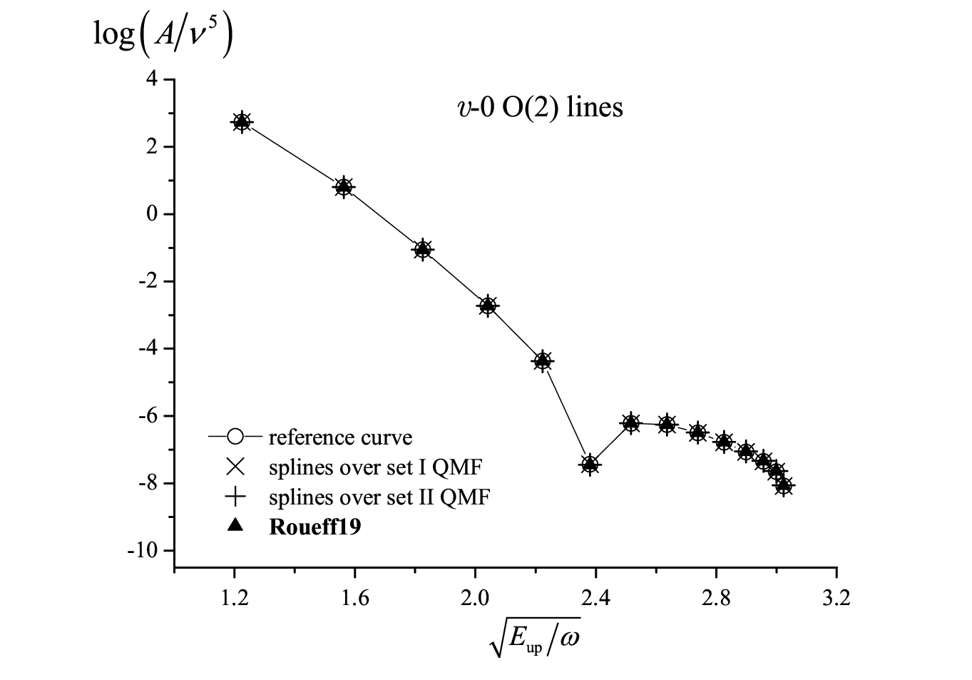
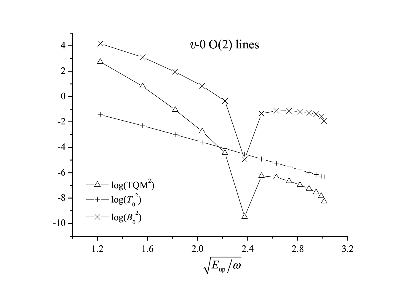
The results for the -0 transitions at -14, i.e. up to the highest bound vibrational level, are shown in Fig. 1 where ratio TQM2 is plotted in the NIDL coordinates because TQM2 is expected to show the NIDL-like behavior (see Sec. 6); this ratio will be called “intensity" for brevity. The calculations were performed with the H2_spectre potential of Komasa19 [6].
First, no signs of saturation is seen.
Second, the sinc-DVR method using the grid of set I ab initio QMF (circles with line), which is considered as “exact" and will be further used as reference, is compared with two other “exact" calculations with use of the set I QMF (crosses) or set II QMF (pluses, previously used in Roueff19) interpolated with splines. The close coincidence of the three calculations suggests that splines do work excellently. It should be noted that in the second and third curves in Fig. 1, as well as in all subsequent calculations, as distinct from the calculation of the first (reference) curve, the Schrödinger equation was solved by the sinc-DVR method using the adaptive analytical mapping approach of Meshkov et al. [37].
Third, our exact sinc-DVR intensity calculations perfectly coincide with the results obtained with the set I spline QMF (crosses) at all transitions including the anomalies (see Sec. 11) at for Q(1) lines and for O(2). Numerically, the differences between sinc-DVR and spline do not exceed 0.001 % at and 0.1–0.4% at .
Thus, we come to the very important conclusions that in H2, as distinct from the molecules with large reduced mass, splines do not deteriorate the high-overtone intensities and that the sinc-DVR method built on the extremely precise ab initio data over the very dense grid is equivalent to the use of a certain analytic function, which is very close, yet not identical, to the true molecular QMF.


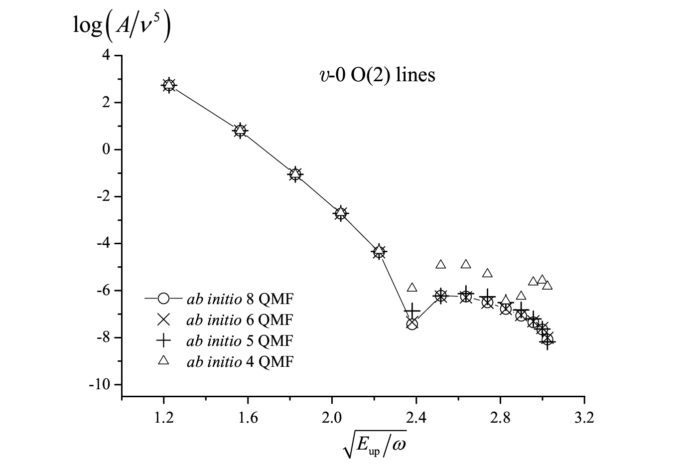
The latter property deserves special consideration. The declared relative accuracy of the ab initio calculated QMF is 10-5 [8], which is equivalent to five significant decimal places. Hence, decimal places 6-8 contain systematic errors associated with the ab initio method used. If one would change the method, a different analytic function would be obtained and then could be used as a comparison function in order to estimate the uncertainties of the calculated intensities.
Here, we explore a different method to construct the comparison functions. First, we introduce random errors into the ab initio QMF by rounding-off the original data to 6, 5, or 4 decimal places in order to determine the actual number of the reliable digits. The results are shown in Fig. 2. It is seen that 6 decimal places is sufficient to recover the data obtained with the original 8-digit QMF; 5 places slightly modify the TQM, and 4 digits destroy it significantly.
6 Method of analysis of the calculated intensities
In our method based on the NIDL theory, the wave functions are written in the quasi-classical form in terms of the classical momenta and actions [12, Appendix]. Then the transition quadrupole moment (TQM) is obtained in the form [13, Eq. (A.2)]
| (4) |
| (5) |
where is the difference between the imaginary parts of the action integrals (in units of ),
| (6) |
in the lower () and upper () states. The integral is taken from a point where the potential is very large, , till the left turning point at a given energy, . Factor is responsible for the NIDL-like decay of the overtone intensities, factor can generate the anomalies. Factor is given by some integral in the complex plane along a contour circumventing the turning points in the upper complex half-plane. The integrand depends on the semiclassical wave functions and on the QMF calculated at the complex points along the integration contour. The explicit expression for is given in [13, Eq. (A.9)].
In fact, as we have demonstrated earlier [12, 13], this quasi-classical method gives practically exact results for heavier molecules, CO and PN. In order to verify the validity of the method in application to a light molecule, H2, we need to compare the calculations using Eqs. (4)-(6) with the exact results obtained by solving the Schrödinger equation. To this end, we used the analytic potential from Piszczatowski09 [4] and the analytically interpolated ab initio QMF of sets I and II, quadr19, to calculate the TQM integral both exactly and quasi-classically, by Eqs. (4)-(6).
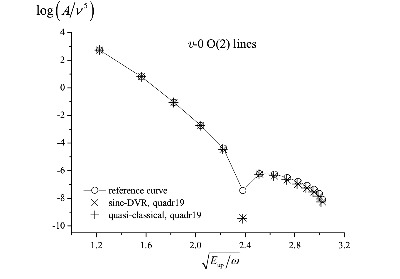
The results are shown in Fig. 3; as in Fig. 1, we divided A (in s-1) by ( is transition frequency in au) because TQM is expected to manifest the NIDL-like dependence in the form of a straight line. The exact calculations are presented by the circles+line data, our reference curve (H2_spectre + sinc-DVR over the set I uniform grid), and also by our model QMF, quadr19, fitted to both sets I and II (crosses). The quasi-classical calculation (pluses) was performed with the same quadr19 QMF. Crosses and pluses are calculated with the Piszczatowski09 [4] potential, which slightly differs from H2_spectre PEF of Komasa19 [6] used for the reference curve.
As is seen in the figure, the quasi-classical method (pluses) is highly accurate, there are no visible differences with the exact calculation (crosses) at the given scale; the differences with the reference curve at the anomalies are due to a different representation of the QMF.
The figure demonstrates once again that replacing splines with an analytic function changes the intensities very insignificantly except for the anomaly. The anomalies (see Sec. 11) are a very special phenomenon because they are highly sensitive to the form of the moment function [38] that is never known for sure; therefore, only experiment can establish which one is closer to the true molecular function than the others. The NIDL predicted by Eqs. (4)-(6) is indeed obeyed except for the anomalies.
As a side result, the effect of the small difference between the potentials of Refs. [4] and [6] on the intensity of the 6-0 O(2) anomaly was estimated to be 10% for the quadr19 QMF.
The above-noted agreement between the quasi-classical and exact results means that the quasi-classical method can be used for the analysis of the calculated data. Yet, in what follows, all the TQM integrals, except where specially noted, are computed exactly, by solving the Schrödinger equation with use of the sinc-DVR method and the analytic functions of Sec. 2 fitted to the data of Sec. 3.


7 Peculiarities of the intensity distribution in H2
In the quasi-classical equations (5) and (6), factor depends only on the repulsive branch of the potential-energy function (PEF), while factor depends on both the PEF and the QMF [12, 13]. In Eq. (4), is responsible for the fast intensity decay with increasing the overtone number whereas is expected to slowly vary with it. This feature was demonstrated for CO [12] and PN [13]. However, in the case of H2, the situation is different.


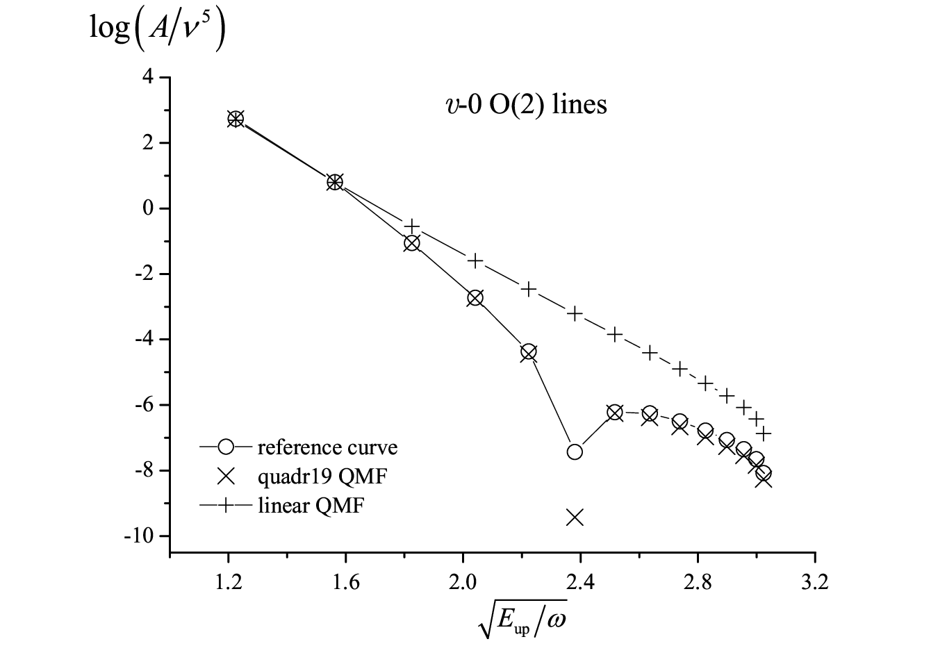
Figure 4 shows the intensities of three lines in the –0 bands, each being calculated with three QMFs, namely, set I QMF as in Fig. 1 (our reference curve) and two analytic functions: the quadr19 QMF and the linear QMF. The latter is expected to show the pure NIDL with no anomalies that usually do not happen with the linear QMFs.
First, we note that all curves indeed manifest the NIDL-like behavior in the form of straight lines except for the anomalies at (the O(2) lines, the reference and quadr19 curves) or at 9-10 (the Q(1) lines, the reference and quadr19 curves). Both the NIDL and the anomalies are in line with the general theory of the intensity distributions in the overtone vibrational spectra [15].
Second, and most importantly, the NIDL slope for the linear QMF is significantly different from two other QMFs, which contradicts to the statement of the general theory [15] that the NIDL slope depends mostly on the potential via factor whereas is a slow function of the overtone number, as took place for CO and PN. In the case of H2, is not a slow function.
In order to demonstrate this explicitly, we plot in Fig. 5 both factors separately for the quadr19 QMF. It is seen that both plots have comparable slopes. This feature deserves special consideration.


Close inspection of the calculated data reveals the reasons for such behavior. The imaginary parts of the classical action entering of Eqs. (5) and (6) is very large, on the order of 1500 and 800 (in units of ) for CO and PN, respectively, whereas it is only about 20 for H2. Two features contribute to this effect: small reduced mass of hydrogen and its less steep potential in the repulsive region. Indeed, the dissociation energy of H2 is about 36118 cm-1 [10], whereas it is about 51000 in PN and 90000 in CO, which means (by analogy with the Morse potential) that the potential of H2 increases more slowly at large and small than those of CO and PN. Also, it looks quite plausible that small number of electrons provides for weaker repulsion/attraction at small/large inter-atomic separations than in many-electron molecules.
As a result of ’s smallness, their difference, , is also small, hence, the steepness of the decay decreases and becomes comparable with that of . Nevertheless, the product of these two factors still obeys the NIDL. Thus, despite the difference of the tunnelling actions is not large, the quasi-classical approximation works perfect in H2 as in other molecules, therefore our method to estimate the expected uncertainties of the calculations can be applied as well.
As a part of our strategy, comparison functions with correct behavior in the complex plane, see [12, 13], have to be constructed that provide for similar NIDLs; then, the remaining differences will serve as estimates of the errors in the calculated intensities. In the case of molecules with heavy atoms, the reference NIDL is that of . As follows from the above consideration, in the case of H2, we should use the full TQM2 (calculated by the sinc-DVR method using the grid of the set I QMF) as reference.
8 Determination of the calculation errors


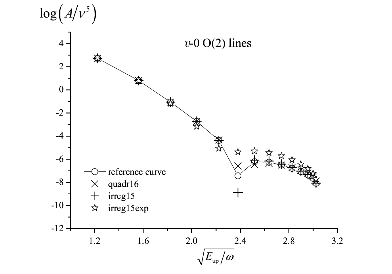
We used our QMFs, Sec. 2 and 4, and the H2_spectre potential-energy function of Komasa19 [6] to calculate the Einstein A coefficients for the X-X ro-vibrational transitions between all bound states of H2. The Schrödinger equation was solved by the sinc-DVR method using the adaptive analytical mapping approach of Meshkov et al. [39].
In Fig. 6, we compare the reference intensities with those calculated with quadr16 and irreg15 fitted to the ab initio data sets I and II, as well as with the irreg15exp QMF fitted not only to sets I and II, but also to the laboratory experimental data, set III. The results for irreg15, quadr16, and irreg15exp are given in supplementary files 4-7.
Obviously, the intensities calculated with all three functions very weakly depend on the QMF form at not very high , namely at for the S(0) lines, for the Q(1) lines, and for the O(2) lines. Even at the highest transitions, the variations of the data obtained with functions irreg15 and quadr16 are within 5–20% over the interval where the intensity itself varies by twelve orders of magnitude. The difference between the results obtained with use of the irreg15exp QMF and the reference curve is larger, it can reach 1-2 orders of magnitude at the highest overtones. Even such values do not seem too large as compared to the variations of the intensity itself, and therefore they could be used to estimate the uncertainties of the calculations. However, it is not clear whether we can trust them because it poorly reproduces the ab initio data.
At this junction, it is important to emphasize that the uncertainty of the set I ab initio QMF declared by Wolniewicz et al. [8] is “likely" to be 10-5 au, as written by the authors, i.e. 100 times smaller than the uncertainty of 0.001 au assigned by us to these data in fitting the irreg15exp QMF. The main reason to consider the irreq15exp QMF is its better reproducing the experimantal data (see Sec. 9).
The other reason can be seen in the figure included in supplementary file 1 where the spline-interpolated set II QMF built on a sparse grid is compared with the set I ab initio QMF over the dense grid. The interpolated QMF closely coincides with the set I QMF at 1-2 au but rapidly declines outside this interval in oscillating manner with the amplitude up to 0.001 au, which could affect the high- transitions; this indeed occurs in CO and PN. In H2, however, the effect is negligible (not shown) because the TQMs themselves are relatively large as compared to the heavier molecules.
The important result is that three functions of very different analytic forms fitted to different data sets give relatively small differences of the intensities of the normal lines in a wide range of transitions, which testifies that all of them, including irreg15exp, approach one and the same true molecular QMF, hence the remaining differences, about one order of magnitude over the 12-orders variations in TQM2, can be interpreted as intrinsic uncertainties of the calculation. If the deviation of 0.001 au from the ab initio QMF is considered impossible, the irreg15exp should be ignored.


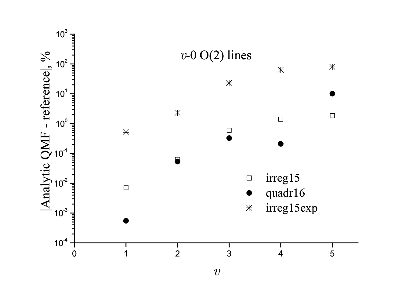
The differences obtained for the low- transitions are explicitly shown in Fig. 7. For irreg15 and quadr16, the differences with the reference values are at the sub-percent level at low ; they increase to a few percent at , as seen in the figure, and to % at (not shown). At the anomalies, the differences reach 1-2 orders of magnitude depending on the anomaly depth. If the irreg15exp is included in comparison, the error at increases up to 60%. These data can be considered as our estimates of the calculation errors.
The calculation errors obtained testify that the estimated current precision of the ab initio calculation exceeds the precision of the experimental measurements of the intensities. The differences of the intensities obtained with use of quadr16 are somewhat larger than with irreg15, probably because the mean-square difference of irreg15 with the ab initio QMF is slightly less than for quadr16. Therefore, we consider irred15 as the best analytic QMF.
The utility of our method to estimate the expected uncertainties of the calculations has been recently demonstrated for CO 7-0 band. In Fig. 8 of our paper [12], the estimated errors of the predicted line intensities in the CO 7-0 band not measured at that time are about 20-30% at , and the measured intensities [40, Table III] are indeed within these limits. In fact, the observed-minus-calculated differences are even smaller, close to the experimental uncertainties.
9 Comparison with the laboratory data

The irreg15 and quadr16 QMFs give the same deviations of the intensities from the laboratory data [24, 9, 30, 31] as those obtained by Roueff19 [10] (not shown).
In Fig. 8 we compare the intensities calculated with the irreg15exp QMF and those of Roueff19 with the laboratory experiments. Since the irreg15exp QMF was fitted not only to sets I and II (the ab initio data of Refs. [8] and [6], respectively), but also to set III (the intensities measured in laboratory), the differences with experiment at –5 are much smaller than those for the data of Roueff et al. who used only set II (their own purely ab initio QMF, Ref. [6]). However, in view of the poor reproduction of the ab initio data mentioned in Sec. 8, we consider the irreg15exp function as inferior as compared to the irreg15 one. Hence, the disagreement with experiment at –5 obtained with our irreg15 and by Roueff et al. should be attributed to the experimental uncertainties as was proposed by Campargue et al. [9].
Comparison of the calculated intensities with the laboratory measurements is given in supplementary files 4-6.
10 Comparison with astrophysical observations
The observations of the H2 emission of space objects bear important spectroscopic information on the vibrational and rotational states, especially on the highly excited states: , with the upper level energies as high as 52000 K, i.e. close to the dissociation limit [3, 33]; [32, 34]; [35]. Even quasi-bound states above the dissociation limit were observed [3] and identified [41]. However, until now, to the best of our knowledge, this information has not been used to verify and improve the theoretical molecular functions of H2. In this section, we summarize the spectroscopic information that can be extracted from the observational data and estimate the relevant uncertainties for their possible use in future refinements of the molecular functions.
The measured -th line flux, , is proportional to the upper-level column density, , and the Einstein coefficient,
| (7) |
where is the line wavelength. For the purpose of astrophysics, this equation is used to derive unknown populations using the calculated values of and [7, 8]. For the purpose of spectroscopy, we can use the ratio of fluxes and emitted from a common upper level with energy in order to derive the observed value of the A ratio,
| (8) |
and then to compare the calculated and observed ratios.
Such comparison is presented in Table 1 for a number of the line pairs observed in emission from various space objects. The observed ratios of were calculated using the integrated line fluxes corrected for the dust extinction that are provided in appropriate references. The calculated ratios were obtained in the present study with use of the H2_spectre PEF [6] and three QMFs, namely, the spline-interpolated ab initio QMF of Wolniewicz et al. [8], quadr16, and irreg15. The data of Roueff et al. [10] were also included. For all lines in Table 1, all four theoretical data sets gave the same ratios within the difference of less than 0.1% (this can be seen below, in Table 3, where the values for some lines calculated with four QMFs are presented). Since the theoretical data were obtained with a number of different QMFs, we conclude that their precision is much higher than that of the observational data, hence the differences between calculations and observations are fully due to the observational errors.
Table 133 3 Table 1 in ASCII format is presented in supplementary file 9. contains the relative difference, , i.e. the observed-minus-calculated ratio divided by the experimental uncertainty. For about a half of the line pairs, it does not greatly exceed unity, hence the theory satisfactorily describes these observational data. For the other half, , which can indicate that the theory needs further refinement. However it should be noted that the observed fluxes include the dust-extinction correction, which is not independently/directly measured. Indeed, there is a number of identical line pairs observed in different sources, they are collected in Table 2, e.g. 6-4 S(0) and 6-4 Q(2). One can see that there is variation of for a given line pair between different observed sources (indicated as err), well beyond the reported uncertainty. In principle this dispersion provides a measure of the systematic uncertainty associated with the dust-extinction correction. Comparing the differences between the calculated and observed ratios with this systematic uncertainty, we see that the theory agrees with the observations (i.e. err) except for three line pairs, namely those with , and 35613. An explanation of this discrepancy can be provided by the relatively coarse spatial resolution of the measurements under consideration. In this case the dust extinction can vary within the point spread function of the telescope. Additionally, it can also vary along each line of sight. We tried to vary the extinction correction for each observed data sets [34, 35, 32], but we could not find an appropriate unique value that could resolve discrepancies for all pair of levels within one data set. Alternatively, the dust-extinction correction can be different for different levels since in principle they can be populated in the different spatial regions of the clouds. Therefore high resolution studies are need to shed light on the observational bias in this problem, which can be done with recently launched James Webb Space Telescope (JWST).
| Line pairs | , K | , m | , obs | , calc | Ref. | |
|---|---|---|---|---|---|---|
| 1-0 Q(2) | 6471 | 2.413439 | 1.199 | 8.7 | [34]∗ | |
| 1-0 S(0) | 2.22329 | |||||
| 1-0 Q(3) | 6951 | 2.42373 | 0.802 | 12.5 | [34]∗ | |
| 1-0 S(1) | 2.121834 | |||||
| 1-0 Q(4) | 7584 | 2.437489 | 0.666 | 12.7 | [34]∗ | |
| 1-0 S(2) | 2.033758 | |||||
| 3-1 O(5) | 17818 | 1.522033 | 0.384 | 0.8 | [34]∗ | |
| 3-2 S(1) | 2.386471 | |||||
| 3-1 O(6) | 18386 | 1.581171 | 0.244 | 0.3 | [34]∗ | |
| 3-2 S(2) | 2.287045 | |||||
| 4-2 O(11) | 27706 | 2.099586 | 0.319 | 0.4 | [34]∗ | |
| 4-3 S(7) | 2.100426 | |||||
| 5-3 O(9) | 30063 | 2.057127 | 0.228 | 0.0 | [34]∗ | |
| 5-3 Q(7) | 1.562635 | |||||
| 6-4 Q(1) | 31063 | 1.601534 | 0.998 | 0.5 | [34]∗ | |
| 6-4 O(3) | 1.732641 | |||||
| 6-4 S(0) | 31304 | 1.536891 | 0.833 | 0.8 | [34]∗ | |
| 6-4 Q(2) | 1.60739 | |||||
| 6-4 S(0) | 31304 | 1.536891 | 0.844 | 1.1 | [34]∗ | |
| 6-4 O(4) | 1.796524 | |||||
| 6-4 Q(2) | 31304 | 1.60739 | 1.013 | 0.6 | [34]∗ | |
| 6-4 O(4) | 1.796524 | |||||
| 6-4 S(1) | 31661 | 1.50156 | 1.249 | 4.8 | [34]∗ | |
| 6-4 Q(3) | 1.616224 | |||||
| 7-5 Q(3) | 35613 | 1.74628 | 0.839 | 1.0 | [34]∗ | |
| 7-5 S(1) | 1.620548 | |||||
| 7-5 O(7) | 36588 | 2.204989 | 0.353 | 0.7 | [34]∗ | |
| 7-5 S(3) | 1.56151 | |||||
| 8-6 O(5) | 39219 | 2.210763 | 0.831 | 0.9 | [34]∗ | |
| 8-6 S(1) | 1.763952 | |||||
| 9-7 Q(1) | 41997 | 2.073187 | 0.863 | 2.1 | [34]∗ | |
| 9-7 O(3) | 2.253724 | |||||
| 9-7 O(4) | 42185 | 2.345581 | 1.596 | 1.6 | [34]∗ | |
| 9-7 S(0) | 1.98735 | |||||
| 9-7 O(4) | 42185 | 2.345581 | 1.211 | 1.9 | [34]∗ | |
| 9-7 Q(2) | 2.084098 | |||||
| 9-7 S(0) | 42185 | 1.98735 | 0.759 | 0.5 | [34]∗ | |
| 9-7 Q(2) | 2.084098 | |||||
| 10-8 S(1) | 45317 | 2.176855 | 1.049 | 0.2 | [34]∗ | |
| 10-7 O(5) | 1.648305 | |||||
| 6-4 S(0) | 31304 | 1.536908 | 0.833 | 7.5 | [35],† A | |
| 6-4 Q(2) | 1.607386 | |||||
| 6-4 Q(1) | 31063 | 1.601535 | 0.998 | 1.9 | [35],† A | |
| 6-4 O(3) | 1.732637 | |||||
| 7-5 S(1) | 35613 | 1.62053 | 1.384 | 4.0 | [35],† A | |
| 7-5 O(5) | 2.02204 | |||||
| 6-4 Q(5) | 32712 | 1.64308 | 2.106 | 3.6 | [35],† A | |
| 6-4 O(7) | 2.029694 | |||||
| 3-1 O(7) | 19086 | 1.645324 | 0.169 | 0.3 | [35],† A | |
| 3-2 S(3) | 2.201397 | |||||
| 11-8 Q(1) | 47391 | 1.657105 | 0.962 | 1.9 | [35],† A | |
| 11-8 O(3) | 1.760929 | |||||
| 4-2 O(7) | 23955 | 1.756296 | 0.408 | 1.8 | [35],† A | |
| 4-3 S(3) | 2.344479 | |||||
| 1-0 S(2) | 7584 | 2.033756 | 1.502 | 5.8 | [35],† A | |
| 1-0 Q(4) | 2.437491 | |||||
| 1-0 S(1) | 6951 | 2.121831 | 1.247 | 8.6 | [35],† A | |
| 1-0 Q(3) | 2.423731 | |||||
| 1-0 S(0) | 6471 | 2.223299 | 0.834 | 4.2 | [35],† A | |
| 1-0 Q(2) | 2.413436 | |||||
| 6-4 S(0) | 31304 | 1.536908 | 0.833 | 0.8 | [35],† B | |
| 6-4 Q(2) | 1.607386 | |||||
| 6-4 Q(1) | 31063 | 1.601535 | 0.998 | 1.5 | [35],† B | |
| 6-4 O(3) | 1.732637 | |||||
| 7-5 S(1) | 35613 | 1.62053 | 1.384 | 2.9 | [35],† B | |
| 7-5 O(5) | 2.02204 | |||||
| 3-1 O(7) | 19086 | 1.645324 | 0.169 | 2.2 | [35],† B | |
| 3-2 S(3) | 2.201397 | |||||
| 4-2 O(7) | 23955 | 1.756296 | 0.408 | 3.0 | [35],† B | |
| 4-3 S(3) | 2.344479 | |||||
| 1-0 S(2) | 7584 | 2.033756 | 1.502 | 13.1 | [35],† B | |
| 1-0 Q(4) | 2.437491 | |||||
| 1-0 S(1) | 6951 | 2.121831 | 1.247 | 5.3 | [35],† B | |
| 1-0 Q(3) | 2.423731 | |||||
| 1-0 S(0) | 6471 | 2.223299 | 0.834 | 6.9 | [35],† B | |
| 1-0 Q(2) | 2.413436 | |||||
| 6-4 Q(1) | 31063 | 1.601535 | 0.998 | 1.5 | [35],† C | |
| 6-4 O(3) | 1.732637 | |||||
| 7-5 S(1) | 35613 | 1.62053 | 1.384 | 4.1 | [35],† C | |
| 7-5 O(5) | 2.02204 | |||||
| 3-1 O(7) | 19086 | 1.645324 | 0.169 | 3.1 | [35],† C | |
| 3-2 S(3) | 2.201397 | |||||
| 4-2 O(7) | 23955 | 1.756296 | 0.408 | 2.7 | [35],† C | |
| 4-3 S(3) | 2.344479 | |||||
| 1-0 S(2) | 7584 | 2.033756 | 1.502 | 21.6 | [35],† C | |
| 1-0 Q(4) | 2.437491 | |||||
| 1-0 S(1) | 6951 | 2.121831 | 1.247 | 5.0 | [35],† C | |
| 1-0 Q(3) | 2.423731 | |||||
| 1-0 S(0) | 6471 | 2.223299 | 0.834 | 3.0 | [35],† C | |
| 1-0 Q(2) | 2.413436 | |||||
| 1-0 S(0) | 6471 | 2.2233 | 0.834 | 15.0 | [32]‡ | |
| 1-0 Q(2) | 2.41344 | |||||
| 1-0 S(1) | 6951 | 2.12183 | 1.247 | 103.5 | [32]‡ | |
| 1-0 Q(3) | 2.42373 | |||||
| 1-0 Q(4) | 7584 | 2.43749 | 0.666 | 33.8 | [32]‡ | |
| 1-0 S(2) | 2.03376 | |||||
| 1-0 Q(5) | 8365 | 2.45475 | 0.605 | 7.3 | [32]‡ | |
| 1-0 S(3) | 1.95756 | |||||
| 2-1 S(3) | 13890 | 2.07351 | 18.404 | 2.1 | [32]‡ | |
| 2-0 O(7) | 1.54641 | |||||
| 3-2 S(1) | 17818 | 2.38645 | 2.602 | 3.6 | [32]‡ | |
| 3-1 O(5) | 1.52203 | |||||
| 3-1 O(7) | 19086 | 1.64532 | 0.169 | 1.4 | [32]‡ | |
| 3-2 S(3) | 2.2014 | |||||
| 1-0 Q(2) | 6471 | 2.4133 | 1.454 | 1.199 | [33],& PK1 | |
| 1-0 S(0) | 2.2235 | |||||
| 1-0 S(1) | 6951 | 2.1218 | 1.006 | 1.247 | [33],& PK1 | |
| 1-0 Q(3) | 2.4237 | |||||
| 1-0 S(2) | 7584 | 2.0334 | 1.02 | 1.502 | [33],& PK1 | |
| 1-0 Q(4) | 2.4375 | |||||
| 1-0 S(3) | 8365 | 1.9576 | 1.875 | 1.653 | [33],& PK1 | |
| 1-0 Q(5) | 2.4547 | |||||
| 1-0 Q(2) | 6471 | 2.4133 | 1.429 | 1.199 | [33],& PK1N | |
| 1-0 S(0) | 2.2235 | |||||
| 1-0 S(1) | 6951 | 2.1218 | 0.951 | 1.247 | [33],& PK1N | |
| 1-0 Q(3) | 2.4237 | |||||
| 1-0 S(2) | 7584 | 2.0334 | 0.95 | 1.502 | [33],& PK1N | |
| 1-0 Q(4) | 2.4375 | |||||
| 1-0 S(3) | 8365 | 1.9576 | 1.981 | 1.653 | [33],& PK1N | |
| 1-0 Q(5) | 2.4547 | |||||
| 1-0 Q(2) | 6471 | 2.4133 | 1.403 | 1.199 | [33],& PK1S | |
| 1-0 S(0) | 2.2235 | |||||
| 1-0 S(1) | 6951 | 2.1218 | 0.998 | 1.247 | [33],& PK1S | |
| 1-0 Q(3) | 2.4237 | |||||
| 1-0 S(2) | 7584 | 2.0334 | 0.982 | 1.502 | [33],& PK1S | |
| 1-0 Q(4) | 2.4375 | |||||
| 1-0 S(3) | 8365 | 1.9576 | 1.736 | 1.653 | [33],& PK1S | |
| 1-0 Q(5) | 2.4547 | |||||
| 1-0 Q(2) | 6471 | 2.4133 | 1.239 | 1.199 | [33],& 118-117 | |
| 1-0 S(0) | 2.2235 | |||||
| 1-0 S(1) | 6951 | 2.1218 | 1.197 | 1.247 | [33],& 118-117 | |
| 1-0 Q(3) | 2.4237 | |||||
| 1-0 S(2) | 7584 | 2.0334 | 1.207 | 1.502 | [33],& 118-117 | |
| 1-0 Q(4) | 2.4375 | |||||
| 1-0 S(3) | 8365 | 1.9576 | 1.761 | 1.653 | [33],& 118-117 | |
| 1-0 Q(5) | 2.4547 | |||||
| 1-0 S(2) | 7584 | 2.0338 | 1.767 | 1.502 | [3]# | |
| 1-0 Q(4) | 2.4375 | |||||
| 1-0 S(1) | 6951 | 2.1218 | 1.251 | 1.247 | [3]# | |
| 1-0 Q(3) | 2.4237 | |||||
| 1-0 S(0) | 6471 | 2.2233 | 1.046 | 0.834 | [3]# | |
| 1-0 Q(2) | 2.4134 | |||||
| a The difference between the theoretical and observational values divided by | ||||||
| the observational error. | ||||||
| ∗ Orion Bar, Kaplan17 [34]. | ||||||
| † NGC 7023, three regions, Le17 [35]. | ||||||
| ‡ Orion KL, Oh16 [32]. | ||||||
| & Orion Molecular Cloud, four regions, Geballe17 [33]. | ||||||
| # Herbig-Haro 7, Pike16 [3]. | ||||||
| Line pairs | , obsa | , calc | No. of entries | ||
| in Table 1 | |||||
| 1-0 Q(2) | 6471 | 1.20 | 0.13 | 10 | |
| 1-0 S(0) | |||||
| 1-0 S(1) | 6951 | 1.25 | 0.16 | 10 | |
| 1-0 Q(3) | |||||
| 1-0 S(2) | 7584 | 1.17 | 1.50 | 0.33 | 10 |
| 1-0 Q(4) | |||||
| 1-0 S(3) | 8365 | 1.79 | 1.65 | 0.14 | 5 |
| 1-0 Q(5) | |||||
| 3-2 S(1) | 17818 | 2.60 | 0.22 | 2 | |
| 3-1 O(5) | |||||
| 3-2 S(3) | 19086 | 5.92 | 1.35 | 4 | |
| 3-1 O(7) | |||||
| 3-2 S(3) | 23955 | 1.59 | 2.45 | 0.86 | 3 |
| 3-1 O(7) | |||||
| 6-4 Q(1) | 31063 | 0.98 | 1.00 | 0.02 | 4 |
| 6-4 O(3) | |||||
| 6-4 Q(2) | 31304 | 1.20 | 0.24 | 4 | |
| 6-4 S(0) | |||||
| 7-5 S(1) | 35613 | 2.53 | 1.38 | 1.15 | 3 |
| 7-5 O(5) | |||||
| a Arithmetic average with scatter, which exceeds the individual | |||||
| uncertainties shown in Table 1. | |||||
| b The maximum and minimum of the observed values are omitted. | |||||
11 Anomalies in the calculated spectra
Anomalies are very common phenomenon in the calculated line lists of diatomic molecules. They appear in the vibrational, vibrational-rotational, and electronic transitions, and some of them were observed in experiment [15, 42, 43].
The rotational anomalies in the electronic spectra were first predicted by Le Roy and coworkers [44, 45] in the vibronic transitions of I2. It was discovered that the Franck-Condon amplitude (the radial overlap integral) as function of crosses zero and changes sign at some , thereby weakening the intensities of the neighboring lines. Such kind of anomalies are also present in the H2 line list recently calculated by Abgrall et al. [46, 47, 48]. While the electronic transitions are beyond the scope of the present paper, there are reasons to discuss them briefly at the end of this section.
The vibrational anomalies in the - transitions were described in Ref. [15]. They arise when the transition moment as function of at fixed crosses zero and changes its sign, thereby making the intensities of the neighboring bands very weak as compared to the values predicted by the NIDL. The vibrational anomalies were predicted in HF [49] and PN [13], predicted and observed in CO [50, 42]. Examples of the H2 vibrational anomalies, 6–0 O(2) and 9–0 Q(1), are shown in Figs. 1-6 above.
The rotational anomalies arise in the vibrational bands of the – transitions when the transition moment changes sign as function of . Examples of the rotational anomalies were given in Refs. [12, Fig. 6] (CO 7-0 R(95)) and [13, Fig. 8 and Table 6] (PN 3-0 P(17), P(18); additionally, the 3-0 band is vibrational anomaly). Recently, a rotational anomaly was observed in the 1-0 band of CH+ [43].
The full list of the vibrational (type “v") and rotational (“r") anomalies in the calculated H2 – vibrational bands is presented in Table 3, of which the full version is given in supplementary file 10. There are also mixed types (“vr") when the TQM changes sign as function of either or . A few interesting features of the data presented in Table 3 deserve special attention.
The calculated intensities of the anomalies depend on the form of the QMF, as is evident from comparison of the intensities calculated in the present study and by Roueff and coauthors. This dependence is much stronger for the anomalies than for the normal lines (not shown). The anomaly position can also change between various QMFs, as demonstrated by two pairs of lines separated by horizontal lines at the bottom of the table.
Especially interesting is the middle part of the table showing the 1.5–2.5 m range where a lot of emission lines has been observed. Some observed lines located near the anomalies are shown in italic along with their calculated values taken from earlier studies in the cited references where available. There are a lot of anomalies in this region, and their coefficients are on the same order as, or 2–4 orders of magnitude lower than, for the neighboring normal lines belonging to various vibrational bands. There are two special examples where the anomalies belong to the same bands as the observed lines: 5-4 S(9) at 2.186 m (anomaly) and 5-4 S(13) at 2.1528 m (observed); 4-3 S(11) at 2 m (anomaly) and 4-3 S(17) at 2.0475 m (observed). In these pairs, the values for the anomalies are only two orders of magnitude weaker than for the observed lines.
Some rotational anomalies that appear in the 1-0 and 2-0 bands are shown in Figs. 9, and 10 along with a few lines observed in space and measured in laboratory. As mentioned above, the values at anomalies are mostly 2-4 orders of magnitude less than at the normal lines within the same band (this is seen in Figs. 9 and 10), which makes them difficult to observe. Yet, there are other factors affecting the observed intensity that vary in wide limits. For instance, the number density in astrophysical objects emitting the H2 lines vary by three orders of magnitude, – cm-3 [34]. The large number of such objects with widely variable conditions give hope that some anomalies could be observed in future, especially with aforementioned JWST.
Figure 11 shows the isotope effect on the 1–0 S(13) anomaly. In HD, the anomaly jumped from to 15, and the intensity dropped down by a few times. Note, however, that HD observations in astrophysical sources is a limiting task, with only a few detections of the strongest line being observed to date.
Figure 12 shows that the magnetic-dipole transitions (with selection rule ) can overlap the anomaly in the Q branch of the electric quadrupole spectrum, thereby making the anomaly not observable.
Sometimes, a special kind of rotational anomaly arises when the transition moment decreases with changing but turns over to increase without changing sign. As shown in Fig. 10, the variation of on the logarithmic scale becomes smooth, therefore we call such an anomaly “flat" as distinct from the “keen", cusp-shaped ones (Figs. 9 and 11) that are due to the sign change of the transition moment. The effect of the TQM sign change at the vibrational anomalies is demonstrated in supplementary file 7 (not shown for the rotational anomalies).
The rest of this section is devoted to vibronic transitions, which seem to be beyond the scope of the present study, so much the more that no relevant calculations were performed by us. The reason to discuss them here is that they contain the keen anomalies (having the beak shape on the semi-logarithmic scale) of exactly the same nature as the keen anomalies in the X–X transitions, namely they all are manifestations of the destructive interference that makes them sensitive to the parameters of the Schrödinger equation.
Figure 13 shows an example of the keen anomaly in the Lyman spectrum calculated by Abgrall et al. [46, 47]. In the footnote to Table II of Ref. [46], the authors write: “Some R and P lines are missing due to weak Franck-Condon factors." These lines missing in the observed spectrum are exactly what Le Roy with coauthors predicted [44, 45], therefore we call such kind of vibronic anomaly the Le Roy anomaly. More such anomalies are presented in supplementary file 11.
Another important features in Fig. 13 are jumps at and 14, which are obviously not the keen anomalies. There are many anomalies of different kinds in the calculated Lyman and Werner bands of H2, e.g. jumps in the values at particular caused by avoided crossings or intensity borrowing [46], yet the keen anomalies deserve special attention. The first key point here is that the keen anomalies are manifestation of a special interference effect. Indeed, when changes, the rotational distortion changes the balance between the positive and negative contributions into the transition integral so that the transition moment can approach and then cross zero at some , – a typical interference phenomenon. And, as a consequence of this destructive interference, the intensity of the weak line, the anomaly, becomes very sensitive to various perturbations. In particular, what can be especially interesting with H2, it can be sensitive to variations of the proton-to-electron mass ratio, .
As we discovered earlier [38], the anomalies are very sensitive to the form of the potential and moment functions. When observed, they could be used, in principle, to improve the theoretical molecular functions. Moreover, they could be also sensitive to the proton-to-electron mass ratio, . These are motivations to discuss here the keen anomalies in more detail.
The search for possible variations of in time or in strong gravitational fields is based on the calculations of line shifts in the observed spectra [2], the respective sensitivity coefficients were calculated in Refs. [37] and [51]. An alternative method could be search of the keen anomalies sensitive to such variations. We did not find any keen anomalies, sensitive enough to , in the H2 – spectrum calculated by Roueff et al. [10], yet this does not mean they do not exist in reality, as discussed below.
By our request, E. Roueff and H. Abgrall made calculations to find a sensitive anomaly in the Lyman band system. Here is citation from Roueff’s letter (bold face are ours). “As you mention in your mail, we indeed find some strong anomalies in the intensities of some electronic transitions of the – system arising from the computations of the transition matrix element and possible cancellation due to destructive interference between the wave functions. These anomalies manifest themselves as huge variations in the transition emission probabilities for which the dependence of the proton-to-electron mass ratio is indeed larger than the mean value. However, the possible experimental or observational measurement seems quite improbable to me. Indeed, for example, we get for –, = 1254.7, = 11, s–1,44 4 Misprint: s-1. a variation in of 2% for = 5e–5." In other words, a relatively huge (in comparison with other studies) variation of resulted in a negligible variation in . The above-mentioned anomaly is shown in Fig. 13.
Our objection to the above reasoning is based on the second key point: The weak sensitivity of the keen anomalies found by us and by the colleagues relates to the artificial theoretical functions rather than the true potential and quadrupole moment, which are unknown. Using the model functions, we can determine only locations and types of the anomalies, but not their precise intensities; the true intensities can differ from the calculated ones by times and orders of magnitude. The sensitivity of the destructive-interference effect to depends on the accuracy with which the interference is complete. When the transition matrix element is extremely small, the sensitivity will be extremely high, and vice versa. Of course, this creates a difficulty to observe such weak lines, but it is a matter of experimental technique, which develops very rapidly towards increasing the measurement precision. When Einstein discovered gravitational waves, he could not imagine that one can ever detect a vibration of a 4th-km-long ruler with the amplitude of a few thousandth of the proton diameter.
Finally, it should be stressed that our classification of the keen anomalies in the vibronic spectra is purely speculative because no calculations on the electronic transitions were made by us in order to determine whether the anomalies shown in Fig. 13 and in supplementary file 11 are indeed associated with the sign change of the TQM. Therefore, before looking for sensitivity of a particular anomaly, one has to verify that the TQM sign change indeed takes place and that, additionally, no stronger magnetic-dipole transition overlaps the given anomaly.
| ) | |||||||
|---|---|---|---|---|---|---|---|
| , s-1 | |||||||
| line | typea | m | irreg15c | ab initio [8]d | ab initio [6]e | Roueff19 [10] | |
| 13-12 O(4) | r | 50995 | 13.536 | 4.8553e-013 | 4.8546e-013 | 4.9091e-013 | 4.382e-013 |
| 13-12 O(3) | v | 50908 | 11.976 | 1.3324e-011 | 1.3324e-011 | 1.3277e-011 | 1.366e-011 |
| 4-1 O(26) | v | 49878 | 2.485 | 2.0469e-009 | 2.0457e-009 | 2.0506e-009 | 2.05e-009 |
| 11-9 S(7) | vr | 50183 | 2.485 | 3.4126e-009 | 3.4147e-009 | 3.429e-009 | 3.483e-009 |
| 7-4 O(20) | v | 49418 | 2.478 | 1.0714e-009 | 1.0726e-009 | 1.0759e-009 | 1.069e-009 |
| 1–0 Q(6)f | 9286 | 2.4755 | Geballe17 [33] | ||||
| 5-2 O(24) | v | 49573 | 2.471 | 3.1231e-009 | 3.1228e-009 | 3.1363e-009 | 3.135e-009 |
| 6-3 O(22) | v | 49420 | 2.467 | 2.868e-009 | 2.8691e-009 | 2.8862e-009 | 2.881e-009 |
| 2-0 O(17) | v | 27265 | 2.458 | 7.0875e-011 | 7.1418e-011 | 7.1424e-011 | 7.203e-011 |
| 1-0 Q(5)f | 2.45475 | Oh16 [32] | |||||
| 11-9 S(6) | v | 49676 | 2.448 | 4.9573e-009 | 4.9553e-009 | 4.9205e-009 | 4.87e-009 |
| 1-0 Q(4)f | 2.437491 | Le17 [35] | |||||
| 11-9 S(5) | v | 49198 | 2.429 | 3.763e-008 | 3.7626e-008 | 3.7488e-008 | 3.739e-008 |
| 6-5 S(7) | r | 35989 | 2.428 | 1.1468e-009 | 1.1475e-009 | 1.1463e-009 | 1.15e-009 |
| 1–0 Q(3)f | 6952 | 2.4237 | Pike16 [3]; A = 2.78e-007 Turner77 [7] | ||||
| 11-9 S(4) | v | 48758 | 2.426 | 9.3066e-008 | 9.3062e-008 | 9.28e-008 | 9.27e-008 |
| 6-5 S(8) | v | 37012 | 2.391 | 1.0786e-008 | 1.0783e-008 | 1.0789e-008 | 1.078e-008 |
| 3–2 S(1)f | 17819 | 2.3863 | Geballe17 [33] | ||||
| 2-0 O(16) | v | 25569 | 2.333 | 1.6751e-010 | 1.6831e-010 | 1.6832e-010 | 1.694e-010 |
| 10-8 Q(2)f | 2.337306 | Le17 [35] | |||||
| 8-5 O(17) | v | 48556 | 2.329 | 4.289e-011 | 4.2562e-011 | 4.3533e-011 | 4.577e-011 |
| 4-1 O(25) | v | 48344 | 2.311 | 2.8962e-009 | 2.8932e-009 | 2.8972e-009 | 2.897e-009 |
| 7-4 O(19) | v | 48267 | 2.303 | 1.9168e-009 | 1.9186e-009 | 1.934e-009 | 1.926e-009 |
| 5-2 O(23) | v | 48158 | 2.298 | 4.5584e-009 | 4.5565e-009 | 4.5702e-009 | 4.569e-009 |
| 6-3 O(21) | v | 48133 | 2.294 | 4.4127e-009 | 4.4134e-009 | 4.4379e-009 | 4.432e-009 |
| 3–2 S(25)f | 51939 | 2.2663 | Pike16 [3]; A = 3.07e-006 Turner77 [7] | ||||
| 5-4 S(9) | vr | 34288 | 2.186 | 5.5675e-009 | 5.568e-009 | 5.5693e-009 | 5.551e-009 |
| 5–4 S(13)f | 39539 | 2.1528 | Pike16 [3]; A = 5.08e-007 Turner77 [7] | ||||
| 8-5 O(16) | v | 47551 | 2.178 | 2.4859e-011 | 2.4549e-011 | 2.3562e-011 | 2.52e-011 |
| 5-4 S(10) | v | 35526 | 2.166 | 5.2832e-008 | 5.283e-008 | 5.2835e-008 | 5.28e-008 |
| 4-1 O(24) | v | 46782 | 2.163 | 3.8428e-009 | 3.8375e-009 | 3.8405e-009 | 3.841e-009 |
| 10-8 S(9) | v | 49541 | 2.161 | 8.0449e-009 | 8.0459e-009 | 8.1621e-009 | 8.225e-009 |
| 7-4 O(18) | v | 47109 | 2.155 | 2.7777e-009 | 2.7797e-009 | 2.8055e-009 | 2.796e-009 |
| 2-1 S(2)f | 2.154225 | Le17 [35] | |||||
| 5-2 O(22) | v | 46721 | 2.151 | 6.1442e-009 | 6.1399e-009 | 6.1515e-009 | 6.15e-009 |
| 6-3 O(20) | v | 46831 | 2.147 | 6.0818e-009 | 6.0812e-009 | 6.1077e-009 | 6.102e-009 |
| 4–3 S(6)f | 26615 | 2.1460 | Geballe17 [33] | ||||
| 10-8 S(8) | vr | 48865 | 2.123 | 4.6464e-009 | 4.6467e-009 | 4.5481e-009 | 4.517e-009 |
| 10-8 S(7) | v | 48213 | 2.098 | 4.936e-008 | 4.9364e-008 | 4.9051e-008 | 4.9e-008 |
| 12-9 S(8) | v | 51947 | 2.086 | 2.983e-009 | 2.9818e-009 | 2.9553e-009 | 2.883e-009 |
| 10-8 S(6) | v | 47595 | 2.085 | 1.3364e-007 | 1.3365e-007 | 1.3321e-007 | 1.332e-007 |
| 10-8 S(5) | v | 47022 | 2.083 | 2.4264e-007 | 2.4265e-007 | 2.422e-007 | 2.423e-007 |
| 2-1 S(3)f | 13890 | 2.073482 | Kaplan17 [34]; A = 5.75e-007 Wolniewicz98 [8] | ||||
| 12-9 O(3)f | 2.069969 | Le17 [35] | |||||
| 8-5 O(15) | v | 46557 | 2.05 | 5.9279e-011 | 5.8746e-011 | 5.5134e-011 | 5.771e-011 |
| 4-1 O(23) | v | 45202 | 2.035 | 4.8545e-009 | 4.8467e-009 | 4.8487e-009 | 4.849e-009 |
| 7-4 O(17) | v | 45954 | 2.028 | 3.4565e-009 | 3.4582e-009 | 3.4886e-009 | 3.478e-009 |
| 5-2 O(21) | v | 45273 | 2.024 | 7.7927e-009 | 7.7854e-009 | 7.7942e-009 | 7.793e-009 |
| 7-5 O(5)f | 2.022040 | Le17 [35] | |||||
| 6-3 O(19) | v | 45524 | 2.02 | 7.71e-009 | 7.7075e-009 | 7.7312e-009 | 7.725e-009 |
| 4-3 S(10) | vr | 31465 | 2.014 | 1.9822e-009 | 1.9848e-009 | 1.9852e-009 | 1.964e-009 |
| 4-3 S(11) | v | 32854 | 2 | 4.1269e-008 | 4.1278e-008 | 4.128e-008 | 4.121e-008 |
| 4–3 S(17)f | 42022 | 2.0475 | Pike16 [3]; A = 1.34e-006 Turner77 [7] | ||||
| 1–0 S(3)f | 8365 | 1.9576 | Geballe17 [33] | ||||
| 10-6 O(16) | v | 51596 | 1.951 | 1.7576e-009 | 1.7603e-009 | 1.74e-009 | 1.722e-009 |
| 2-1 S(5)f | 1.94487 | Oh16 [32] | |||||
| 8-5 O(14) | v | 45584 | 1.938 | 2.4683e-010 | 2.4572e-010 | 2.3574e-010 | 2.412e-010 |
| 9-7 S(11) | v | 48987 | 1.937 | 2.1414e-008 | 2.1409e-008 | 2.1622e-008 | 2.168e-008 |
| 4-1 O(22) | v | 43612 | 1.923 | 5.8951e-009 | 5.885e-009 | 5.8862e-009 | 5.887e-009 |
| 7-4 O(16) | v | 44812 | 1.917 | 3.7642e-009 | 3.7651e-009 | 3.7937e-009 | 3.783e-009 |
| 5-2 O(20) | v | 43822 | 1.912 | 9.4048e-009 | 9.3943e-009 | 9.4005e-009 | 9.399e-009 |
| 6-3 O(18) | v | 44223 | 1.909 | 9.1162e-009 | 9.1112e-009 | 9.1298e-009 | 9.123e-009 |
| 9-7 S(10) | vr | 48144 | 1.897 | 9.0535e-010 | 9.0694e-010 | 8.7707e-010 | 8.722e-010 |
| 9-7 S(9) | v | 47318 | 1.869 | 4.1735e-008 | 4.1747e-008 | 4.1656e-008 | 4.167e-008 |
| 3-2 S(11) | vr | 28555 | 1.868 | 2.6272e-010 | 2.6385e-010 | 2.6398e-010 | 2.542e-010 |
| 3-2 S(12) | v | 30097 | 1.858 | 2.9354e-008 | 2.9366e-008 | 2.9367e-008 | 2.927e-008 |
| 9-7 S(8) | v | 46521 | 1.85 | 1.3711e-007 | 1.3713e-007 | 1.3716e-007 | 1.373e-007 |
| 9-7 S(7) | v | 45762 | 1.84 | 2.7337e-007 | 2.734e-007 | 2.7365e-007 | 2.739e-007 |
| 8-5 O(13) | v | 44641 | 1.839 | 9.0176e-010 | 8.9977e-010 | 8.7895e-010 | 8.895e-010 |
| 4-1 O(21) | v | 42020 | 1.823 | 6.9242e-009 | 6.9123e-009 | 6.913e-009 | 6.915e-009 |
| 7-4 O(15) | v | 43693 | 1.819 | 3.5617e-009 | 3.5615e-009 | 3.584e-009 | 3.573e-009 |
| 5-2 O(19) | v | 42377 | 1.813 | 1.0871e-008 | 1.0858e-008 | 1.0862e-008 | 1.086e-008 |
| 6-3 O(17) | v | 42936 | 1.811 | 1.0114e-008 | 1.0107e-008 | 1.012e-008 | 1.012e-008 |
| 10-6 O(15) | v | 50921 | 1.802 | 3.1503e-009 | 3.155e-009 | 3.1701e-009 | 3.149e-009 |
| 11-8 S(10) | v | 51758 | 1.794 | 9.4044e-009 | 9.4071e-009 | 9.263e-009 | 9.173e-009 |
| 11-8 O(3)f | 1.760929 | Le17 [35] | |||||
| 8-5 O(12) | v | 43739 | 1.752 | 2.669e-009 | 2.6661e-009 | 2.6315e-009 | 2.651e-009 |
| 2-1 S(12) | r | 25569 | 1.742 | 5.3761e-011 | 5.3882e-011 | 5.3859e-011 | 5.93e-011 |
| 2-1 S(13) | v | 27265 | 1.736 | 1.809e-008 | 1.809e-008 | 1.809e-008 | 1.8e-008 |
| 4-1 O(20) | v | 40433 | 1.734 | 7.896e-009 | 7.8833e-009 | 7.8837e-009 | 7.885e-009 |
| 6-4 O(3)f | 1.732637 | Le17 [35] | |||||
| 8-6 S(12) | vr | 47551 | 1.732 | 1.4013e-009 | 1.3982e-009 | 1.3851e-009 | 1.38e-009 |
| 7-4 O(14) | v | 42605 | 1.731 | 2.8123e-009 | 2.811e-009 | 2.8261e-009 | 2.816e-009 |
| 5-2 O(18) | v | 40946 | 1.725 | 1.2074e-008 | 1.2059e-008 | 1.2062e-008 | 1.206e-008 |
| 6-3 O(16) | v | 41671 | 1.724 | 1.053e-008 | 1.052e-008 | 1.0529e-008 | 1.052e-008 |
| 1-0 S(8)f | 1.71466 | Oh16 [32] | |||||
| 8-6 S(11) | v | 46557 | 1.701 | 2.1541e-008 | 2.1551e-008 | 2.1668e-008 | 2.172e-008 |
| 10-6 O(14) | v | 50231 | 1.681 | 4.1372e-009 | 4.143e-009 | 4.2133e-009 | 4.191e-009 |
| 8-6 S(10) | v | 45584 | 1.678 | 1.0572e-007 | 1.0573e-007 | 1.0607e-007 | 1.062e-007 |
| 2-0 O(9)f | 15763 | 1.679641 | Kaplan17 [34]; A = 1.29e-008 Wolniewicz98 [8] | ||||
| 8-6 S(9) | v | 44641 | 1.663 | 2.4328e-007 | 2.4329e-007 | 2.4382e-007 | 2.442e-007 |
| 11-8 Q(1)f | 1.657105 | Le17 [35] | |||||
| 8-6 S(8) | v | 43739 | 1.654 | 4.1862e-007 | 4.1862e-007 | 4.1926e-007 | 4.198e-007 |
| 7-4 O(13) | v | 41558 | 1.653 | 1.6498e-009 | 1.648e-009 | 1.6563e-009 | 1.648e-009 |
| 4-1 O(19) | v | 38859 | 1.653 | 8.7593e-009 | 8.747e-009 | 8.7472e-009 | 8.749e-009 |
| 5-2 O(17) | v | 39537 | 1.645 | 1.2892e-008 | 1.2876e-008 | 1.2878e-008 | 1.288e-008 |
| 6-3 O(15) | v | 40438 | 1.644 | 1.0219e-008 | 1.0207e-008 | 1.0213e-008 | 1.02e-008 |
| 1-0 S(11)f | 18979 | 1.650413 | Kaplan17 [34]; A = 5.37e-008 Wolniewicz98 [8] | ||||
| 1-0 S(13) | r | 22516 | 1.632 | 4.5463e-010 | 4.5889e-010 | 4.5886e-010 | 4.735e-010 |
| 1-0 S(14) | v | 24367 | 1.63 | 8.16e-009 | 8.1445e-009 | 8.1446e-009 | 8.087e-009 |
| 7-5 S(14) | v | 47109 | 1.607 | 1.5097e-008 | 1.5088e-008 | 1.4966e-008 | 1.492e-008 |
| 10-7 S(12) | v | 51596 | 1.6 | 1.0993e-008 | 1.1001e-008 | 1.0923e-008 | 1.087e-008 |
| 7-5 S(2)f | 1.588290 | Le17 [35] | |||||
| 7-4 O(12) | v | 40559 | 1.582 | 4.6704e-010 | 4.6559e-010 | 4.6875e-010 | 4.635e-010 |
| 10-6 O(13) | v | 49541 | 1.58 | 4.3071e-009 | 4.3126e-009 | 4.4248e-009 | 4.403e-009 |
| 4-1 O(18) | v | 37306 | 1.579 | 9.4571e-009 | 9.4464e-009 | 9.4466e-009 | 9.445e-009 |
| 7-5 S(13) | vr | 45954 | 1.575 | 3.8377e-009 | 3.8403e-009 | 3.9022e-009 | 3.939e-009 |
| 6-3 O(14) | v | 39245 | 1.573 | 9.1045e-009 | 9.0927e-009 | 9.0965e-009 | 9.086e-009 |
| 5-2 O(16) | v | 38158 | 1.572 | 1.3204e-008 | 1.3189e-008 | 1.319e-008 | 1.319e-008 |
| 5-3 O(2)f | 26606 | 1.560736 | Kaplan17 [34]; A = 2.24E-006 Wolniewicz98 [8] | ||||
| 7-5 S(12) | v | 44812 | 1.549 | 5.9038e-008 | 5.9038e-008 | 5.9247e-008 | 5.943e-008 |
| 12-7 O(12) | v | 51947 | 1.54 | 8.3512e-010 | 8.3761e-010 | 8.4954e-010 | 8.323e-010 |
| 7-5 S(11) | v | 43693 | 1.53 | 1.7356e-007 | 1.7354e-007 | 1.7383e-007 | 1.742e-007 |
| 3-1 O(5)f | 1.52203 | Oh16 [32] | |||||
| 7-4 O(11) | vr | 39618 | 1.518 | 2.3598e-011 | 2.4024e-011 | 2.3508e-011 | 2.47e-011 |
| 7-5 S(10) | v | 42605 | 1.516 | 3.3583e-007 | 3.3578e-007 | 3.3607e-007 | 3.366e-007 |
| 5-3 Q(4)f | 1.515792 | Le17 [35] | |||||
| 4-1 O(17) | v | 35783 | 1.511 | 9.9274e-009 | 9.9198e-009 | 9.92e-009 | 9.922e-009 |
| 4-2 O(3)f | 22079 | 1.509865 | Kaplan17 [34]; A = 7.76e-007 Wolniewicz98 [8] | ||||
| 7-5 S(9) | v | 41558 | 1.508 | 5.3073e-007 | 5.3065e-007 | 5.309e-007 | 5.317e-007 |
| 6-3 O(13) | v | 38100 | 1.507 | 7.2187e-009 | 7.2077e-009 | 7.2101e-009 | 7.202e-009 |
| 5-2 O(15) | v | 36818 | 1.506 | 1.2904e-008 | 1.289e-008 | 1.2891e-008 | 1.289e-008 |
| 6-4 S(1)f | 31661 | 1.50156 | Kaplan17 [34]; A = 1.15e-006 Wolniewicz98 [8] | ||||
| 10-6 O(12) | v | 48865 | 1.496 | 3.5165e-009 | 3.5203e-009 | 3.6386e-009 | 3.619e-009 |
| 6-4 S(15) | vr | 45524 | 1.477 | 1.2438e-009 | 1.2444e-009 | 1.2239e-009 | 1.198e-009 |
| 9-6 S(14) | v | 51507 | 1.463 | 6.435e-009 | 6.4423e-009 | 6.5505e-009 | 6.547e-009 |
| 12-3 O(2) | v | 49354 | 0.45 | 1.6556e-011 | 1.1558e-011 | 1.1441e-011 | 1.111e-011 |
| 8-1 O(2) | v | 38604 | 0.448 | 1.2222e-011 | 7.4728e-012 | 7.7483e-012 | 8.672e-012 |
| 10-2 O(2) | v | 44819 | 0.44 | 2.3926e-011 | |||
| 11-1 Q(2) | v | 47535 | 0.35 | 1.6571e-014 | |||
| 9-0 Q(4) | v | 42827 | 0.35 | 1.8971e-014 | |||
| 11-1 Q(1) | v | 47391 | 0.349 | 1.1775e-016 | |||
| 9-0 Q(3) | vr | 42463 | 0.347 | 9.1824e-016 | |||
| 9-0 Q(2) | v | 42185 | 0.345 | 3.1132e-015 | 1.9326e-014 | 1.5311e-014 | 1.521e-014 |
| 9-0 Q(1) | v | 41998 | 0.344 | 1.8542e-014 | 8.6009e-015 | 5.3482e-015 | 5.269e-015 |
| 12-1 Q(4) | vr | 49932 | 0.34 | 5.3309e-016 | |||
| 12-1 Q(3) | v | 49706 | 0.337 | 3.75e-014 | |||
| 12-1 Q(3) | vr | 49706 | 0.337 | 3.7163e-015 | 2.0719e-015 | 3.778e-015 | |
| 10-0 Q(6) | vr | 46500 | 0.334 | 3.263e-016 | |||
| 12-1 Q(2) | v | 49532 | 0.334 | 5.5923e-015 | 8.9173e-015 | 6.355e-015 | |
| 13-1 Q(5) | vr | 51473 | 0.334 | 2.0924e-015 | |||
| 12-1 Q(1) | v | 49414 | 0.333 | 3.9967e-014 | 5.1183e-014 | 5.132e-014 | |
| 10-0 Q(5) | v | 46038 | 0.33 | 8.2368e-015 | 2.2102e-015 | ||
| 10-0 Q(5) | vr | 46038 | 0.33 | 1.2674e-15 | 1.2410e-15 | ||
| 13-1 Q(4) | vr | 51284 | 0.329 | 3.6783e-016 | 8.77e-016 | 8.85e-016 | |
| 10-0 Q(4) | v | 45641 | 0.327 | 2.6532e-015 | 4.3113e-015 | 4.381e-015 | |
| 10-0 Q(3) | v | 45317 | 0.325 | 1.8397E-14 | 2.3179E-14 | 2.3380E-14 | |
| 11-0 Q(7) g | vr | 49198 | 0.323 | 1.8539e-015 | |||
| 11-0 Q(6) | vr | 48758 | 0.318 | 1.1498e-15 | 2.0069E-15 | 2.0410E-15 | |
| 12-0 Q(8) g | vr | 51218 | 0.317 | 7.4371e-016 | |||
| 12-0 Q(7) | vr | 50856 | 0.311 | 8.7092e-16 | 1.4616E-15 | 1.4800E-15 | |
| a Anomaly types: v, vibrational; r, rotational; vr, vibrational-rotational (see text). | |||||||
| b The energy of the upper state in Kelvin. | |||||||
| c Present study, the irreg15 TQM. | |||||||
| d Present study, the spline-interpolated ab initio TQM of Wolniewicz [8]. | |||||||
| e Present study, the spline-interpolated TQM of Komasa19 [6]. | |||||||
| f Observed lines near the anomalies are shown in italic. The reference to the source | |||||||
| is given. The calculated values for these lines from the source are cited. | |||||||
| g When QMF is changed, the anomaly can disappear (empty spaces) or move to a neighbouring | |||||||
| (two examples are shown by horizontal lines.) | |||||||


12 Conclusions
This study was motivated by the fact that the X-X ro-vibrational transition intensities were calculated with use of the spline-interpolated quadrupole-moment function (QMF) [10], which had been compromised in CO [11, 52] and other molecules [14]. The second motivation was that the numerous available experimental and observational data were not used in construction of the QMF. In order to resolve these issues, we constructed a few analytic functions fitted to either the ab initio data only or to both the ab initio and experimental data. We used these analytic QMFs to calculate the transition intensities and found the following.
1. In the case of H2, as distinct from other molecules, the use of the spline-interpolated QMF does not deteriorate the overtone intensities and does not lead to nonphysical saturation owing to the high precision of the ab initio data (at least six decimal places) and the high density of the ab initio grid.
2. The use of the laboratory data does not help increase the quality of the analytic QMF. While the observed-minus-calculated differences can be essentially decreased by fitting the QMF to the experimental data, this is reached by a large deviation of the QMF from the ab initio data that seems improbable.
3. The same is true of the astrophysical observations in view of low precision of the data, since there is likely large systematic uncertainties are associated with the dust extinction.
4. The theoretical A values are used in astrophysics to determine the column densities for individual lines and the temperature of the emitting objects [3, 34, 41, 35, 33, 53]. Our new data do not affect the results of this analysis.
5. The NIDL theory applies to H2, i.e. the transition moment is factorised as , where is the exponential factor depending on the potential alone and pre-factor depending on both the potential and the QMF. As always, the pre-factor is responsible for the anomalies, i.e. the lines with intensities lower than those predicted by the NIDL for the “normal" lines. The anomalies arise because can cross zero and change its sign at some transitions. The difference with other molecules is that is no longer a slow function of the overtone number as compared to , therefore it affects the NIDL slope.
6. Numerous anomalies resulting from destructive interference (the “keen" anomalies) are identified in the calculated line lists. Some of them are situated within the recently observed spectral regions, e.g. 1.5-2.5 m, and some are close to such regions. The intensities of the anomalies are very sensitive to the QMF representation, as illustrated by comparison of our results with those of Roueff et al. [10].
7. As a side result, we mention the Le Roy anomalies in the ro-vibronic (electronic) spectra of H2. Le Roy with co-authors [44, 45] predicted that the transition matrix element of I2 can cross zero as function of and change its sign, exactly as in our case of the X-X transitions. Here, we demonstrated that numerous Le Roy anomalies are seen in the Lyman and Werner series.
8. Since the keen anomalies in both the vibration-rotation and vibronic spectra are sensitive to the potential and the moment, we assumed that they might be also sensitive to the proton-to-electron mass ratio. Sample calculations by us as well as by E. Roueff and H. Abgrall performed by our request (unpublished) did reveal enhanced sensitivity of the anomalies as compared to the normal lines, yet insufficient to be observed.
9. The insensitivity of the keen anomalies relates to the model molecular functions whereas the actual functions can make some anomalies sensitive. The only thing that theory can do is to predict the position of the anomaly; one also has to make sure that the particular anomaly is due to the sign change of the transition matrix element in order that the anomaly were of the interference nature.
Supplementary material
File 1 Comparing sets I and II QMFs.pdf.
File 2 H2_laboratory_data.txt.
File 3 QMFs_em.f. FORTRAN codes for three analytic quadrupole-moment functions: irreg15, irreg16, and irreg15exp.
File 4 Fit_OUT_Irreg15_Paper_em1.txt. The output file for the FORTRAN code using irreg15.
File 5 Fit_OUT_Quadr16_Paper_em.txt. The output file for the FORTRAN code using quadr16.
File 6 Fit_TDM_DMF-0_001_em1.txt. The output file for the FORTRAN code using irreg15exp.
File 7 TQMs_em.txt. The transition quadrupole moments computed with three QMFs for the S(0), Q(1), and O(2) lines at .
File 8 parameters_em.txt. The fitted parameters of the irreg15, irreg15exp, and quadr16 QMFs.
File 9 H2_astrophysical_data_Table1.txt.
File 10 Paper_on_H2_2023_Table3_full.pdf.
Acknowledgements
We are grateful to J. Komasa for ab initio data, E. Roueff and H. Abgrall for the calculations discussed in Sec. 11. The work by VGU and ESM was carried out in accordance with the state task, state registration number AAAA-A19-119071190017-7.
References
- [1] I. E. Gordon, L. S. Rothman, R. J. Hargreaves, R. Hashemi, E. V. Karlovets, F. M. Skinner, E. K. Conway, C. Hill, R. V. Kochanov, Y. Tan, P. Wcisło, A. A. Finenko, K. Nelson, P. F. Bernath, M. Birk, V. Boudon, A. Campargue, K. V. Chance, A. Coustenis, B. J. Drouin, J.-M. Flaud, R. R. Gamache, J. T. Hodges, D. Jacquemart, E. J. Mlawer, A. V. Nikitin, V. I. Perevalov, M. Rotger, J. Tennyson, G. C. Toon, H. Tran, V. G. Tyuterev, E. M. Adkins, A. Baker, A. Barbe, E. Canè, A. G. Cs’asz’ar, A. Dudaryonok, O. Egorov, A. J. Fleisher, H. Fleurbaey, A. Foltynowicz, T. Furtenbacher, J. J. Harrison, J.-M. Hartmann, V.-M. Horneman, X. Huang, T. Karman, J. Karns, S. Kassi, I. Kleiner, V. Kofman, F. Kwabia-Tchana, N. N. Lavrentieva, T. J. Lee, D. A. Long, A. A. Lukashevskaya, O. M. Lyulin, V. Y. Makhnev, W. Matt, S. T. Massie, M. Melosso, S. N. Mikhailenko, D. Mondelain, H. S. P. M"uller, O. V. Naumenko, A. Perrin, O. L. Polyansky, E. Raddaoui, P. L. Raston, Z. D. Reed, M. Rey, C. Richard, R. T’obi’as, I. Sadiek, D. W. Schwenke, E. Starikova, K. Sung, F. Tamassia, S. A. Tashkun, J. Vander Auwera, I. A. Vasilenko, A. A. Vigasin, G. L. Villanueva, B. Vispoel, G. Wagner, A. Yachmenev, S. N. Yurchenko, The HITRAN2020 molecular spectroscopic database, Journal of Quantitative Spectroscopy and Radiative Transfer 277 (2022) 107949. doi:10.1016/j.jqsrt.2021.107949.
- [2] W. Ubachs, J. Bagdonaite, E. J. Salumbides, M. T. Murphy, L. Kaper, Colloquium: Search for a drifting proton-electron mass ratio from , Rev. Mod. Phys. 88 (2016) 021003. doi:10.1103/RevModPhys.88.021003.
- [3] R. E. Pike, T. R. Geballe, M. G. Burton, A. Chrysostomou, Highly excited H2 in Herzberg-Haro 7: Formation pumping in shocked molecular gas?, Astrophys. J. 822 (2016) 82 (13pp). doi:10.3847/0004-637X/822/2/82.
- [4] K. Piszczatowski, G. Łach, M. Przybytek, J. Komasa, K. Pachucki, B. Jeziorski, Theoretical Determination of the Dissociation Energy of Molecular Hydrogen, J. Chem. Theory Comp. 5 (2009) 3039–3048. doi:10.1021/ct900391p.
- [5] K. Pachucki, Born-Oppenheimer potential for H2, Phys. Rev. A 82 (2010) 032509. doi:10.1103/PhysRevA.82.032509.
- [6] J. Komasa, M. Puchalski, P. Czachorowski, G. Łach, K. Pachucki, Rovibrational energy levels of the hydrogen molecule through nonadiabatic perturbation theory, Phys. Rev. A 100 (2019) 032519. doi:10.1103/PhysRevA.100.032519.
- [7] J. Turner, K. Kirby-Docken, A. Dalgarno, The quadrupole vibration-rotation transition probabilities of molecular hydrogen, Astrophys. J. Suppl. Ser. 35 (1977) 281–292.
- [8] L. Wolniewicz, I. Simbotin, A. Dalgarno, Quadrupole transition probabilities for the excited rovibrational states of H2, Astrophys. J. Suppl. Ser. 115 (2) (1998) 293–313. doi:10.1086/313091.
- [9] A. Campargue, S. Kassi, K. Pachucki, J. Komasa, The absorption spectrum of H2: CRDS measurements of the (2-0) band, review of the literature data and accurate ab initio line list up to 35000 cm-1, Phys. Chem. Chem. Phys. 14 (2012) 802–815. doi:10.1039/c1cp22912e.
- [10] E. Roueff, H. Abgrall, P. Czachorowski, K. Pachucki, M. Puchalski, J. Komasa, The full infrared spectrum of molecular hydrogen, A&A 630 (2019) A58. doi:10.1051/0004-6361/201936249.
- [11] E. S. Medvedev, V. V. Meshkov, A. V. Stolyarov, I. E. Gordon, Peculiarities of high-overtone transition probabilities in carbon monoxide revealed by high-precision calculation, J. Chem. Phys. 143 (16) (2015) 154301. doi:10.1063/1.4933136.
- [12] E. S. Medvedev, V. G. Ushakov, Irregular semi-empirical dipole-moment function for carbon monoxide and line lists for all its isotopologues verified for extremely high overtone transitions, J. Quant. Spectrosc. Radiat. Transfer 288 (2022) 108255. doi:10.1016/j.jqsrt.2022.108255.
- [13] V. G. Ushakov, M. Semenov, S. N. Yurchenko, A. Y. Ermilov, E. S. Medvedev, Improved potential-energy and dipole-moment functions of the ground electronic state of phosphorus nitride, J. Mol. Spectrosc. 395 (2023) 111804. doi:10.1016/j.jms.2023.111804.
- [14] E. S. Medvedev, V. G. Ushakov, Selection of the model functions for calculations of high-overtone intensities in the vibrational-rotational spectra of diatomic molecules, Opt. spectrosc. 130 (9) (2022) 1334–1342. doi:10.21883/OS.2022.09.53292.3428-22[inRussian.Englishtranslationisavailableatdoi:10.21883/EOS.2022.09.54822.3428-22].
- [15] E. S. Medvedev, Towards understanding the nature of the intensities of overtone vibrational transitions, J. Chem. Phys. 137 (2012) 174307. doi:10.1063/1.4761930.
- [16] U. Fink, T. A. Wiggins, D. H. Rank, Frequency and intensity measurements on the quadrupole spectrum of molecular hydrogen, J. Mol. Spectrosc. 18 (4) (1965) 384–395. doi:10.1016/0022-2852(65)90044-5.
- [17]
J. S. Margolis,
Measurement
of some 1-0 H2 quadrupole transition strengths, J. Mol. Spectrosc.
48 (2) (1973) 409–410.
doi:https://doi.org/10.1016/0022-2852(73)90203-8.
URL https://www.sciencedirect.com/science/article/pii/0022285273902038 - [18] C. Chackerian, L. P. Giver, Density-dependent frequency shift of the hydrogen S2(1) quadrupole line, J. Mol. Spectrosc. 58 (3) (1975) 339–343. doi:10.1016/0022-2852(75)90215-5.
- [19] C. Chackerian, L. P. Giver, Measurement of weak ir absorption with a tunable laser: the hydrogen S2(1) line strength, Applied Optics 14 (8) (1975) 1993–1996. doi:10.1364/AO.14.001993.
- [20] J. T. Bergstralh, J. W. Brault, Intensity and pressure shift of H2 (4,0) S(1) quadrupole line, Astrophys. J. 224 (1978) L39–L41.
- [21] J. Reid, A. R. W. McKellar, Observation of the pure rotational quadrupole transition of with a tunable diode laser, Phys. Rev. A 18 (1978) 224–228. doi:10.1103/PhysRevA.18.224.
- [22] J. T. Trauger, M. E. Mickelson, L. E. Larson, Laboratory absorption strengths for the H2 (4,0) and (3,0) S(1) lines, Astrophys. J. 225 (1978) L157–L160.
- [23] J. W. Brault, W. H. Smith, Determination of the H2 4-0 S(1) quadrupole line strength and pressure shift, Astrophys. J. 235 (1980) L177–L178.
- [24] S. L. Bragg, J. W. Brault, W. H. Smith, Line positions and strengths in the h2 quadrupole spectrum, Astrophys. J. 263 (1982) 999–1004.
- [25] D. E. Jennings, J. W. Brault, The Ground State of Molecular Hydrogen, Astrophys. J. 256 (1982) L29–L31.
- [26] D. W. Ferguson, K. N. Rao, M. E. Mickelson, L. E. Larson, An Experimental Study of the 4-0 and 5-0 Quadrupole Vibration Rotation Bands of H2 in the Visible, J. Mol. Spectrosc. 160 (2) (1993) 315–325. doi:10.1006/jmsp.1993.1178.
- [27] D. C. Reuter, J. M. Sirota, Astrophys. J. 428 (1994) L77–L79.
- [28] M. Gupta, T. Owano, S. Baer, D, A. O’Keefe, Quantitative determination of the Q(1) quadrupole hydrogen absorption in the near infrared via off-axis ICOS, Chem. Phys. Lett. 418 (1) (2006) 11–14. doi:10.1016/j.cplett.2005.10.081.
- [29] D. C. Robie, J. T. Hodges, Line positions and line strengths for the electric quadrupole band of H, J. Chem. Phys. 124 (2006). doi:10.1063/1.2145925.
- [30] S.-M. Hu, H. Pan, C.-F. Cheng, Y. R. Sun, X.-F. Li, J. Wang, A. Campargue, A.-W. Liu, The S(0)-S(3) electric quadrupole transitions of H2 near 0.8 m, Astrophys. J. 749 (2012) 76. doi:10.1088/0004-637X/749/1/76.
- [31] S. Kassi, A. Campargue, Electric quadrupole transitions and collision-induced absorption in the region of the first overtone band of H2 near 1.25 m, J. Mol. Spectrosc. 300 (2014) 55–59. doi:10.1016/j.jms.2014.03.022.
- [32] H. Oh, T.-S. Pyo, K. Kaplan, I.-S. Yuk, B.-G. Park, G. Mace, C. Park, M.-Y. Chun, S. Pak, K.-M. Kim, J. S. Oh, U. Jeong, Y. S. Yu, J.-J. Lee, H. Kim, N. Hwang, H.-I. Lee, H. A. N. Le, S. Lee, D. T. Jaffe, Three-dimensional shock structure of the orion kl outflow with igrins, Astrophys. J. 833 (2016) 275. doi:10.3847/1538-4357/833/2/275.
- [33] T. R. Geballe, M. G. Burton, R. E. Pike, Very High Excitation Lines of H2 in the Orion Molecular Cloud Outflow, Astrophys. J. 837 (2017) 83 (7pp). doi:10.3847/1538-4357/aa619e.
- [34] K. F. Kaplan, H. L. Dinerstein, H. Oh, G. N. Mace, H. Kim, K. R. Sokal, M. D. Pavel, S. Lee, S. Pak, C. Park, J. Sok Oh, D. T. Jaffe, Excitation of Molecular Hydrogen in the Orion Bar Photodissociation Region from a Deep Near-infrared IGRINS Spectrum, Astrophys. J. 838 (2017) 152 (13pp). doi:10.3847/1538-4357/aa5b9f.
- [35] H. A. N. Le, S. Pak, K. Kaplan, G. Mace, S. Lee, M. Pavel, U. Jeong, H. Oh, H.-I. Lee, M.-Y. Chun, I.-S. Yuk, T.-S. Pyo, N. Hwang, K.-M. Kim, C. Park, J. Sok Oh, Y. S. Yu, B.-G. Park, Y. C. Minh, D. T. Jaffe, Fluorescent H2 Emission Lines from the Reflection Nebula NGC 7023 Observed with IGRINS, Astrophys. J. 841 (2017) 13 (18pp). doi:10.3847/1538-4357/aa6bf7.
- [36] K. Pachucki, J. Komasa, Magnetic dipole transitions in the hydrogen molecule, Phys. Rev. A 83 (2011) 032501. doi:10.1103/PhysRevA.83.032501.
- [37] V. V. Meshkov, A. V. Stolyarov, A. V. Ivanchik, D. A. Varshalovich, Ab initio nonadiabatic calculation of the sensitivity coefficients for the ; lines of H2 to the proton-to-electron mass ratio, JETP Lett. 83 (2006) 303–307. doi:10.1134/S0021364006080017.
- [38] E. S. Medvedev, V. G. Ushakov, High sensitivity of the anomalies in the rotational and ro-vibrational bands of carbon monoxide to small changes in the molecular potential and dipole moment, J. Mol. Spectrosc. 349 (2018) 60–64. doi:10.1016/j.jms.2018.04.008.
- [39] V. V. Meshkov, A. V. Stolyarov, R. J. Le Roy, Adaptive analytical mapping procedure for efficiently solving the radial Schrödinger equation, Phys. Rev. A 78 (2008) 052510. doi:10.1103/PhysRevA.78.052510.
- [40] A. A. Balashov, K. Bielska, G. Li, A. A. Kyuberis, S. Wójtewicz, J. Domysławska, R. Ciuryło, N. F. Zobov, D. Lisak, J. Tennyson, O. L. Polyansky, Measurement and calculation of CO (7-0) overtone line intensities, J. Chem. Phys. 158 (2023) 234306. doi:10.1063/5.0152996.
- [41] E. Roueff, M. G. Burton, T. R. Geballe, H. Abgrall, Analysis of the first infrared spectrum of quasi-bound H2 line emission in Herbig-Haro 7, Astronomy & Astrophysics (2023, manuscript no. 45358arxaa).
- [42] C.-Y. Chung, J. F. Ogilvie, Y.-P. Lee, Detection of Vibrational-Rotational Band 0-3 of 12C16O with Cavity Ringdown Absorption near 0.96 m, J. Phys. Chem. A 109 (2005) 7854–7858. doi:10.1021/jp052035x.
- [43] P. B. Changala, D. A. Neufeld, B. Godard, Anomalous Intensities in the Infrared Emission of CH+ Explained by Quantum Nuclear Motion and Electric Dipole Calculations, Astrophys. J. 917 (2021) 16. doi:10.3847/1538-4357/ac05c8.
- [44] J. D. Brown, G. Burns, R. J. Le Roy, Improved spectroscopic data synthesis for I and predictions of dependence for transition intensities, Can. J. Phys. 51 (1973) 1664–1677.
- [45] R. J. Le Roy, E. R. Vrscay, Periodicity of the oscillatory dependence of diatomic molecule Franck–Condon factors, Canad. J. Phys. 53 (16) (1975). doi:10.1139/p75-198.
- [46] H. Abgrall, E. Roueff, F. Launay, J.-Y. Roncin, J.-L. Subtil, The Lyman and Werner Band Systems of Molecular Hydrogen, J. Mol. Spectrosc. 157 (1993) 512–523. doi:10.1006/jmsp.1993.1040.
- [47] H. Abgrall, E. Roueff, F. Launay, J.-Y. Roncin, J.-L. Subtil, The Lyman Band Systems of Molecular Hydrogen, Astron, Astrophys. Suppl. Ser. 101 (1993) 273–321.
- [48] H. Abgrall, E. Roueff, F. Launay, J.-Y. Roncin, J.-L. Subtil, The Werner Band Systems of Molecular Hydrogen, Astron, Astrophys. Suppl. Ser. 017 (1993) 323–362.
- [49] R. E. Meredith, F. G. Smith, Computation of electric dipole matrix elements for hydrogen fluoride, J. Quant. Spectrosc. Radiat. Transfer 13 (1973) 89–114. doi:10.1016/0022-4073(73)90105-2.
- [50] E. Medvedev, Determination of a new molecular constant from overtone vibrational spectra, J. Mol. Spectrosc. 114 (1985) 1–12. doi:10.1016/0022-2852(85)90330-3.
- [51] E. J. Salumbides, J. Bagdonaite, H. Abgrall, E. Roueff, W. Ubachs, H2 Lyman and Werner band lines and their sensitivity for a variation of the proton-electron mass ratio in the gravitational potential of white dwarfs, Mon. Not. Royal Astr. Soc. 450 (2015) 1237–1245. doi:10.1093/mnras/stv656.
- [52] E. S. Medvedev, V. V. Meshkov, A. V. Stolyarov, V. G. Ushakov, I. E. Gordon, Impact of the dipole-moment representation on the intensity of high overtones, J. Mol. Spectrosc. 330 (2016) 36–42. doi:10.1016/j.jms.2016.06.013.
- [53] D. A. Neufeld, B. Godard, P. B. Changala, A. Faure, T. R. Geballe, R. Gusten, K. M. Menten, H. Wiesemeyer, Observations and analysis of CH+ vibrational emissions from the young, carbon-rich planetary nebula NGC 7027: A textbook example of chemical pumping, Astrophys. J. 917 (2021) 15. doi:10.3847/1538-4357/ac05c9.