Pseudo Flow Consistency for Self-Supervised 6D Object Pose Estimation
Abstract
Most self-supervised 6D object pose estimation methods can only work with additional depth information or rely on the accurate annotation of 2D segmentation masks, limiting their application range. In this paper, we propose a 6D object pose estimation method that can be trained with pure RGB images without any auxiliary information. We first obtain a rough pose initialization from networks trained on synthetic images rendered from the target’s 3D mesh. Then, we introduce a refinement strategy leveraging the geometry constraint in synthetic-to-real image pairs from multiple different views. We formulate this geometry constraint as pixel-level flow consistency between the training images with dynamically generated pseudo labels. We evaluate our method on three challenging datasets and demonstrate that it outperforms state-of-the-art self-supervised methods significantly, with neither 2D annotations nor additional depth images.
1 Introduction
The goal of 6D object pose estimation is to accurately estimate the 3D rotation and 3D translation of a rigid object with respect to the camera, which gives essential information about the world beyond classical 2D understanding and is a fundamental component in many applications, such as robotic manipulation [5], autonomous driving [36], and augmented reality [37].
Recent progress in this field has significantly improved the robustness and accuracy of the model [49, 60, 21, 56, 7, 29, 19, 18]. Most of these approaches, however, rely on a large number of real images with accurate 6D pose annotations. But, compared to classical 2D annotation, these 6D annotations are either very hard to obtain [38, 34] or are prone to contain large labeling errors [16, 11, 58].
Some recent methods propose to use techniques based on image synthesis [15] or self-supervised learning [55, 54] to handle this problem. The main problem with synthetic images is the large domain gap to the real images, making the model’s generalization ability suffers in practice [42, 60]. On the other hand, most self-supervised methods rely on additional information. Some can only work with additional depth images [55, 54, 31, 4] or others need pixel-level annotation of a segmentation mask [46, 61], which prevents the general applicability, as shown in Fig. 1.
 |
| (a) Existing self-supervised 6D object pose methods |
 |
| (b) Our solution based on pseudo flow consistency |
 |
 |
| (a) The standard strategy for self-supervised classification | (b) The proposed strategy for self-supervised object pose estimation |
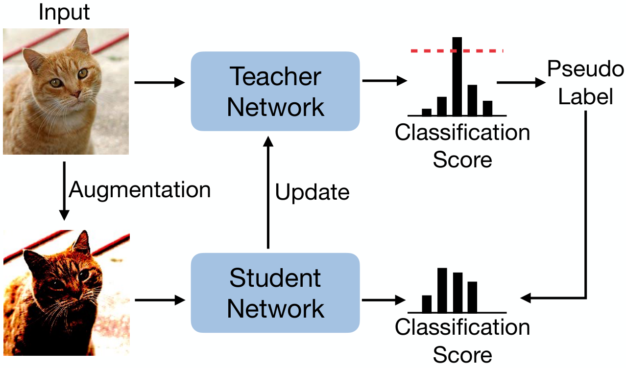
In this work, we propose a self-supervised framework for 6D object pose estimation, which relies on neither depth nor additional 2D annotations. We first generate a synthetic dataset based on rendered images from the target’s 3D mesh and train networks only on this dataset to get a rough pose initialization. To close the domain gap between the synthetic and real data, we use a refinement strategy where we compare the rendered reference image according to the initial pose and the real input based on pseudo labels [47, 62]. Pseudo labeling is widely used in many computer vision tasks [52, 59, 12, 8]. However, the two fundamental problems of pseudo labeling are still open questions in 6D object pose estimation, including the generative strategy of creating pseudo labels and the selection strategy of extracting high-quality labels from the noisy candidates, as shown in Fig. 2.
We propose to formulate the pseudo 6D pose labels as pixel-level flow supervision signals in a render-and-compare framework [16, 26, 29, 60, 21, 32, 9]. Unlike the common render-and-compare frameworks that need accurate pose annotations, we propose a geometry-guided learning framework without any annotations. We render multiple images near the initial pose, and compare them with the real input with the guidance of flow consistency, based on the geometry constraints between these image pairs from different views. We choose high-quality flow labels based on the proposed consistency on the fly, and supervise the network training with these dynamically generated labels in every training step.
We evaluate our method on three challenging datasets LINEMOD [14], Occluded-LINEMOD [24], and YCB-V [58], and show that it outperforms state-of-the-art self-supervised methods significantly, including those methods relied on depth image [55, 54] or auxiliary annotation information [61, 46].
Our contributions can be summarized as the following. First, we investigate the problem of the standard teacher-student methods in selecting high-quality pseudo labels for self-supervised object pose estimation. Second, we propose a strategy based on flow consistency that embeds the geometry constraint from multiple views. Finally, we demonstrate its effectiveness by significantly outperforming state-of-the-art self-supervised object pose methods, without relying on any auxiliary information.

2 Related Work
Object pose estimation has shown significant progress recently, based on different techniques, such as direct pose regression [56, 7, 26], 2D reprojection regression [44, 42, 18, 19, 40], 3D keypoint prediction [30, 41, 49, 11], and differentiable PnP solver [27, 17, 2, 3]. However, most of these methods rely on a large number of real images with accurate 6D pose annotation, which is usually hard to obtain in practice, especially in cluttered scenes with multiple object instances and occlusions [58, 16].
Some recent methods tackle this problem by training on synthetic images rendered from the target’s 3D mesh [11, 42, 1], but this strategy suffers from the domain gap between the synthetic and real image sets [6]. In contrast, some pose refinement methods have shown significant improvement in the generalization ability across different domains [29, 32, 26, 21, 60, 9] and especially [16], which produces comparable results as the state-of-the-art methods with only about one-tenth of the real images involved in training. Although having this promising progress, these pose refinement methods still need many annotated real images for training, and can not easily benefit from more real data without further annotations.
To solve this problem, some recent self-supervised methods [55, 61, 46, 54] try to remove the cumbersome procedure of pose annotation completely. Most of them are based on a strategy that compares the synthetic image rendered from an initial pose with the real image, and backpropagate the gradient through a differentiable renderer [23, 33] to update the network’s weights during training, expecting to align the rendered image with the real input without explicit annotations. This type of strategy, however, relies heavily on the performance of comparing the final rendered image and the real input, which suffers from the domain gap, making them often rely either on depth [55] or on additional pixel-level annotations of segmentation masks [61]. In contrast, we propose to compare multiple synthetic-to-real image pairs at the same time, and force networks to comply with the geometry constraint between those image pairs from different views, which suffers little from the domain problem. On the other hand, we formulate the geometry constraint as pixel-level consistency, which provides us dynamic valid label mask during training, without any 3D depth information or additional 2D mask annotations.
Pseudo labeling is also one of the basic techniques used in recent self-supervised object pose methods [31, 4]. However, these approaches still rely on additional depth images to select valid pseudo labels. In addition, they only update the pseudo labels after finishing the previous training, which usually means the model needs to be trained multiple times to utilize the slowly updated pseudo labels. By contrast, our pseudo flow labels are generated dynamically in every training step, and our model only needs to be trained once.
Our method is related to the recent teacher-student formulation of pseudo labeling [47, 62, 52, 59, 25, 64, 28, 63, 57, 43, 22], which works under the assumption that the generated high-quality pseudo label of the teacher can be used to supervise the student network when having the same input as the teacher but only different data augmentations. Although this simple general framework has been widely used in image classification [47, 62], object detection [59, 28, 64, 51], and semantic segmentation [25], it only can work with high-quality pseudo labels. However, there is still no easy way to generate high-quality pose labels in the context of 6D object pose estimation. To solve this problem, we propose to formulate pseudo 6D pose labels as pixel-level flow supervision signals and select high-quality pseudo flow labels based on flow consistency across multiple different views during training. Our experiments demonstrate the effectiveness of this method.
3 Approach
Given a dataset of calibrated RGB images and the 3D mesh of the target, our goal is to train a self-supervised model on this dataset to estimate the 6D object pose of the target, without relying on depth images or any auxiliary information, such as 6D pose and 2D mask annotations. We first create a synthetic dataset by rendering the 3D mesh of the target in different poses and train an existing pose estimation network [19, 26] on it to obtain a rough pose initialization [16, 29, 21]. The core component of our method is a self-supervised pose refinement framework, which we will discuss in detail in this section. We first show an overview of our self-supervised framework, and then present how we formulate the flow consistency based on the geometry constraint between different views. Finally, we show how we extend it to multiple image pairs to further increase the robustness. Fig. 3 shows the overview of our method.
 |
 |
| (a) Flow consistency across multiple views | (b) Flow-guided photometric consistency |
3.1 Framework Overview
We use a teacher-student architecture [52] for our self-supervised framework. It contains two networks with identical network structures, but not shared weights, which are called the teacher and student, respectively. During training, when an image input of the teacher network can produce a prediction that can fulfill some criteria, we convert this prediction to a one-hot pseudo-label, and use it to supervise the student network with the same image input but only different data augmentations. After updating the weights of the student network by gradient backpropagation supervised by this pseudo label, we then update the weights of the teacher network by a simple exponential moving averaging (EMA) strategy from the student network:
| (1) |
where and are the network weight parameters of the teacher and student network, respectively, and is the exponential factor, which is typically 0.999. The weight updating and pseudo label generation is conducted after each iteration during training, making it much more efficient than other pseudo-label-based object pose methods [4, 31], which can only produce pseudo labels after the whole training pipeline and need to train the model multiple times.
Our main problem is how to select high-quality pseudo label candidates from the noisy predictions of the teacher network. For the image classification task as in [52], one can obtain the label quality by the output distribution after the softmax operation easily, which is usually implemented by checking if the probability of any class is above a threshold [47, 62]. However, there is no such easy way to determine the quality of an object pose prediction without the ground truth. We discuss our solution in the following sections.
3.2 Flow Consistency across Multiple Views
To solve the problem of difficulties in determining the quality of object pose predictions, we first formulate object pose estimation as a problem of estimating dense 2D-to-2D correspondence, or optical flow estimation, as in PFA [16], which, however, is a fully-supervised object pose method. To tackle the problem of no pose annotation for the computation of ground truth flow, we render multiple images around the initial pose, and predict the flow between each of them and the real input. In principle, since both the rendered images and real input image are 2D reprojections of the same 3D object, the flow prediction that aligns with the underlying geometry should have a higher probability of being of high quality. Fig. 4(a) illustrates such consistency assumption.
More formally, given an unannotated real image and the obtained initial pose from networks trained only on synthetic data, we randomly generate another poses , around the initial pose , and then create synthetic images by rendering the target under the corresponding poses, generating image pairs:
| (2) |
where is the rendered image of the target under pose .
For an object having 3D keypoints, the 2D reprojection of a 3D keypoint under pose can be obtained by
| (3) |
where is a scale factor, is the 2D image location, is the intrinsic camera matrix, and and are the rotation and translation of pose , respectively. We then establish 3D-to-2D correspondence under pose . For the real image , although its true pose is unknown to us, the relation between the 3D keypoint and its 2D image location should follow the perspective principle of Eq. 3, implicitly generating the correspondence .
We train a network to predict dense 2D-to-2D correspondence between the two images in each image pair of Eq. 2, such that
| (4) |
where is the corresponding 2D flow vector. Although is unknown during training, we have the geometry constraint that the 2D image locations of the same 3D keypoint from different synthetic views should be the same.
We use the standard variance of the predicted from different views to determine if the current pixel’s flow prediction is a valid pseudo label
| (5) |
and select valid flow pseudo labels by a simple threshold . Fig. 7 shows some visualizations of the variance .
After obtaining the valid flow labels from the teacher network, we use them to supervise the student network by a loss function
| (6) |
where is the flow network with parameters and for the teacher and student network, respectively, and is the same real image as but only with different data augmentations, and is the mask containing valid pixels where . Note that, is generated dynamically from the consistency check between multiple image pairs in Eq. 2, and does not rely on any 2D mask annotations.
3.3 Flow-Guided Photometric Consistency
The previous section only investigates the consistency between the synthetic views and the real input. We further explore the consistency between multiple real inputs. Our motivation is that the 2D image reprojections of the same 3D object keypoint on different real images should have similar textures. We formulate this texture assumption as a photometric consistency, as illustrated in Fig. 4(b).
Given the real image with the initial pose , as in the previous section, we randomly retrieve another real images whose initial pose is around , generating image pairs
| (7) |
and after feeding the two images in each image pair to the teacher network, we have
| (8) |
where is the predicted 2D image location on image . We assume these predicted 2D image locations of the same 3D keypoint have similar texture properties, and we use a photometric loss to model this
| (9) |
where is an operation function that warps the image according to the new pixel locations, is a generalized Charbonnier function to measure the photometric difference based on the Census transformation [39], and is inferred from the student’s prediction, where
| (10) |
We combine the flow consistency and photometric consistency into our final loss
| (11) |
Note that, we only apply the loss to the student network since the gradient backprogataion only occurs for the student network, and the teacher network only gets its weight updated by EMA updating as discussed in Section 3.1.
4 Experiments
In this section, we first present the experiment setting of our method and then compare our method with state-of-the-art self-supervised methods. We finally conduct detailed ablation studies of our method in various settings. Our source code is publicly available at https://github.com/YangHai-1218/PseudoFlow.
4.1 Experiment Setup
Datasets. We evaluate our method on three widely-used datasets for 6D object pose estimation: LINEMOD (“LM”) [14], Occluded-LINEMOD (“LM-O”) [24], and YCB-V [58]. LINEMOD dataset contains 13 objects, with a single sequence per object without occlusions. We follow [55, 16] to use 15% of the real images for training, resulting in a total of 2.4k images. Occluded-LINEMOD is an extension of LINEMOD, which annotates all the objects in one sequence in LINEMOD as the test set and shares the training set with LINEMOD. The recent YCB-V dataset consists of 130k real training images for 21 texture-less objects captured in cluttered scenes. Although all these three datasets contain manually labeled annotations, we train our models on them without accessing the ground truth, and report the final accuracy on their test set. We use the synthetic dataset used in the BOP challenge [6, 15, 50] to train WDR-Pose [19] for the pose initialization.
Evaluation Metrics. We mainly use ADD-0.1d as our metric, which computes the average distance between the mesh vertices transformed by the predicted pose and the ground truth pose, and then only treat the prediction with an average 3D error below 10% of the mesh diameter as a correct pose estimate. We use its symmetric version for symmetric objects. Additionally, in some settings, we also use BOP metrics [15] for evaluation, including the Visible Surface Discrepancy (VSD), the Maximum Symmetry-aware Surface Distance (MSSD), the Maximum Symmetry-aware Projection Distance (MSPD), and their average AR. We refer the readers to [15] for their detailed definition.
Training details. We use RAFT [53] as our flow network for both the teacher and student network. We initialize the weights of both teacher and student network with the weights pretrained on synthetic data and train the model using AdamW optimizer [35] with a batch size of 16. We use One-cycle strategy [45] to anneal the learning rate from a starting point 4e-4. We crop the target object from the original image according to the initial pose, and then resize the image patch to 256256. We do not use any data augmentation in the teacher network, and only use random color augmentation used in PFA [16] for the student network. We typically set , , and in our experiments. Unlike [55, 54, 31, 20] that train a separate model for each object, which is cumbersome to train, we train a single model for all objects in the same dataset.
4.2 Comparison against State of the Art
We first compare our method against the state-of-the-art self-supervised pose estimation methods on LINEMOD and Occluded-LINEMOD. Since most of them report numbers only in ADD-0.1d, we follow the same for a fair comparison. Table. 1 and 2 summarize the result. Our method outperforms the state-of-the-art methods significantly. Especially, our method, which requires only RGB images, even outperforms Self6D [54] by 3.7% on LINEMOD, which is a method that relies on additional depth images. We show some qualitative results in Fig. 5.
| Method | DSC [61] | Sock et al. [46] | Lin et al. [31] | Self6D [54] | Self6D [54] | Ours |
| Ape | 31.2 | 37.6 | 67.5 | 76.0 | 75.4 | 81.9 |
| Bench. | 83.0 | 78.6 | 99.9 | 91.6 | 94.9 | 95.0 |
| Cam | 49.6 | 65.6 | 87.4 | 97.1 | 97.0 | 94.2 |
| Can | 56.5 | 65.6 | 99.2 | 99.8 | 99.5 | 96.8 |
| Cat | 57.9 | 52.5 | 94.3 | 85.6 | 86.6 | 95.4 |
| Driller | 73.7 | 48.8 | 97.6 | 98.8 | 98.9 | 94.8 |
| Duck | 31.3 | 35.1 | 67.2 | 56.5 | 68.3 | 83.5 |
| Eggbox* | 96.0 | 89.2 | 98.9 | 91.0 | 99.0 | 93.9 |
| Glue* | 63.4 | 64.5 | 96.2 | 92.2 | 96.1 | 96.5 |
| Holep. | 38.8 | 41.5 | 49.9 | 35.4 | 41.9 | 84.5 |
| Iron | 61.9 | 80.9 | 99.5 | 99.5 | 99.4 | 94.9 |
| Lamp | 64.7 | 70.7 | 99.8 | 97.4 | 98.9 | 94.8 |
| Phone | 54.4 | 60.5 | 91.5 | 91.8 | 94.3 | 94.1 |
| Avg. | 58.6 | 60.6 | 88.4 | 85.6 | 88.5 | 92.2 |
| Method | DSC [61] | Sock et al. [46] | Lin et al. [31] | Self6D [54] | Self6D [54] | Ours |
| Ape | 9.1 | 12.0 | 40.3 | 57.7 | 59.4 | 60.1 |
| Can | 21.1 | 27.5 | 75.2 | 95.0 | 96.5 | 94.2 |
| Cat | 26.0 | 12.0 | 35.0 | 52.6 | 60.8 | 56.5 |
| Driller | 33.5 | 20.5 | 68.5 | 90.5 | 92.0 | 89.7 |
| Duck | 12.2 | 23.0 | 25.7 | 26.7 | 30.6 | 30.9 |
| Eggbox* | 39.4 | 25.1 | 44.7 | 45.0 | 51.1 | 58.1 |
| Glue* | 37.0 | 27.0 | 60.7 | 87.1 | 88.6 | 88.9 |
| Holep. | 20.4 | 35.0 | 28.0 | 23.5 | 38.5 | 44.2 |
| Avg. | 24.8 | 22.8 | 47.3 | 59.8 | 64.7 | 65.4 |
4.3 Ablation Study
Evaluation of different components. Table. 3 summarizes the results of our method with different components. The first row is the results of the standard teacher-student structure used in [47]. Although it has the standard EMA updating strategy, its performance is limited, mainly caused by the lacking of high-quality pseudo pose labels. After adding our flow loss and photometric loss, the performance increases significantly, which demonstrates the effectiveness of the proposed components.
Training analysis on YCB-V. We evaluate our method in three different settings during the training, as shown in Fig. 6. The baseline is the original teacher-student structure [52], and the other two are the proposed components of our method. The baseline model struggles to learn from the unannotated data without explicit quality measurement of pseudo labels. Our flow loss introduces a constraint based on flow consistency derived from multiview geometry, and tackles this problem effectively, and the proposed photometric loss increases performance further, as shown in Fig. 7.
| MSPD | MSSD | VSD | ADD | ||
| - | - | 0.759 | 0.589 | 0.519 | 30.9 |
| - | ✓ | 0.765 | 0.631 | 0.578 | 37.5 |
| ✓ | - | 0.780 | 0.711 | 0.658 | 64.2 |
| ✓ | ✓ | 0.785 | 0.749 | 0.664 | 67.4 |
| Method | MSPD | MSSD | VSD | ADD |
| Initialization v1 | 0.632 | 0.491 | 0.420 | 27.4 |
| + Ours (Real) | 0.780 | 0.731 | 0.673 | 64.6 |
| + Ours (SSL) | 0.759 | 0.722 | 0.650 | 63.2 |
| Initialization v2 | 0.673 | 0.580 | 0.508 | 36.0 |
| + Ours (Real) | 0.775 | 0.722 | 0.660 | 65.3 |
| + Ours (SSL) | 0.764 | 0.724 | 0.643 | 64.2 |
| Initialization v3 | 0.694 | 0.598 | 0.522 | 38.6 |
| + Ours (Real) | 0.803 | 0.752 | 0.686 | 69.2 |
| + Ours (SSL) | 0.785 | 0.749 | 0.664 | 67.4 |
 |
 |
 |
 |
 |
 |
 |
 |
 |
 |
 |
 |
 |
 |
 |
 |
 |
 |
 |
|
 |
 |
 |
 |
 |
 |
 |
|
| Input | Variance | Flow error | |||||
| (a) Ablation study in ADD-0.1d and AR | (b) Different amount of real training data | |
Evaluation of hyper-parameters. We evaluate the hyper-parameters used in our framework in Fig. 8. We first evaluate the impact of the number of different views. More views generally increase the performance, since it adds more information to the geometry constraint. However, too many views, such as those larger than 4, has negative impacts on the performance. We believe it is caused by the noise introduced by too many views with large viewpoint differences, which usually makes the network harder to learn. We then evaluate the threshold used in our framework, which is used to determine the reliability of pseudo flow labels. It works well between 1 and 4.
Evaluation with limited real data. We evaluate our method on YCB-V with different amounts of real data used in training, as shown in Fig. 8(b). Our method increases the performance by about 20.2% (from 41.7% to 61.9%) in ADD-0.1d by only using 1% of all the real data. 99% more real data can only increase the performance by 5.5% further, which demonstrates the effectiveness of our method in data-limited scenarios.
Evaluation with different initialization and additional annotations. In principle, our method can be trained with ground truth pose annotations easily, which is basically training the student network in a standard fully-supervised way. We evaluate our self-supervised method with the version trained with real pose annotations. At the same time, to evaluate the robustness of our framework to different pose initialization, we evaluate three versions of pose initialization with different initialization accuracy, including the results obtained by the original WDR-Pose, and two other versions with pre-cropping the detected regions of interest, based on Mask RCNN [13] and RADet [10], respectively. Table 4 summarizes the results. Although the initial poses have different accuracy, our self-supervised refinement framework boosts their performance significantly, and even achieves similar performance as that trained on fully-annotated real images.
Comparison against standard optical flow methods. In principle, one can use a self-supervised optical flow method to directly establish dense 2D-to-2D correspondence between the rendered image and the real image input, without any real pose annotations. However, we find that this strategy hardly can work, mainly due to the large domain gap between the rendered and real images, in which case the standard component of photometric comparison in self-supervised flow methods suffers. We evaluate a typical self-supervised optical flow method SMURF [48], and report the results on YCB-V in Table 5. Our self-supervised strategy suffers little from this domain gap problem and produces much more accurate pose results than SMURF.
| Method | MSPD | MSSD | VSD | ADD |
| SMURF [48] | 0.751 | 0.565 | 0.488 | 28.7 |
| Ours | 0.785 | 0.749 | 0.664 | 67.4 |
 |
 |
 |
 |
 |
 |
 |
 |
| Symmetry objects | Ground truth | Initialization | Refinement |
Symmetry handling. We use the same strategy as in [16, 44] for symmetric objects in obtaining pose initialization, which restricts the range of poses used in training depending on the objects’ symmetry type. We do not explicitly handle the symmetry for the refinement, where we build multiple views around the initial pose and use the consistency constraint between them to find the best flow to align different views within a small pose range. Fig. 9 shows two examples with reflectional symmetry and rotational symmetry, respectively. Note how the predicted poses have different 3D axis from the ground truth pose but align the target mesh with the images well in appearance.
Time analysis. We conduct all our experiments on a workstation with an NVIDIA RTX-3090 GPU and an Intel-Xeon CPU with 12 cores running at 2.1GHz. The training of our self-supervised framework is only about 20% slower than its fully-supervised version, consuming about 30 and 24 hours in the typical setting on YCB-V, respectively, which is much more efficient than methods relying on multiple times of retraining [31, 4]. For the inference time, our method is the same as its fully-supervised version and takes only 23ms for a single object, including the optical flow estimation 17ms and the PnP solver 6ms.
5 Conclusion
We have introduced a simple self-supervised 6D object pose method. After obtaining the rough pose initialization based on a network training on synthetic images, we refine the pose with a teacher-student pseudo labeling framework. To solve the problem of identifying high-quality labels in the context of object pose estimation, we first formulate pseudo object pose labels as pixel-level optical flow supervision signals. Then, we introduce a flow consistency based on the underlying geometry constraint between multiple different views. Our experiments show that the proposed method significantly outperforms existing solutions in both accuracy and efficiency, without relying on any 2D annotations or additional depth images.
Acknowledgments. This work was supported by the Natural Science Foundation of China, the Youth Innovation Team of Shaanxi Universities, the Fundamental Research Funds for the Central Universities under Grant JBF220101, and the 111 Project of China under Grant B08038. We thank Thomas Probst, Daniel Koguciuk, Juan-Ting Lin, and Lin Sun for helpful discussions.
References
- [1] Dingding Cai, Janne Heikkilä, and Esa Rahtu. SC6D: Symmetry-agnostic and Correspondence-free 6D Object Pose Estimation. In International Conference on 3D Vision, 2022.
- [2] Bo Chen, Alvaro Parra, Jiewei Cao, Nan Li, and Tat-Jun Chin. End-to-End Learnable Geometric Vision by Backpropagating PnP Optimization. In Conference on Computer Vision and Pattern Recognition, 2020.
- [3] Hansheng Chen, Pichao Wang, Fan Wang, Wei Tian, Lu Xiong, and Hao Li. EPro-PnP: Generalized End-to-End Probabilistic Perspective-n-Points for Monocular Object Pose Estimation. In Conference on Computer Vision and Pattern Recognition, 2022.
- [4] Kai Chen, Rui Cao, Stephen James, Yichuan Li, Yun-Hui Liu, Pieter Abbeel, and Qi Dou. Sim-to-Real 6D Object Pose Estimation via Iterative Self-training for Robotic Bin Picking. In European Conference on Computer Vision, 2022.
- [5] Alvaro Collet, Manuel Martinez, and Siddhartha S Srinivasa. The MOPED Framework: Object Recognition and Pose Estimation for Manipulation. The international journal of robotics research, 30(10):1284–1306, 2011.
- [6] Maximilian Denninger, Martin Sundermeyer, Dominik Winkelbauer, Dmitry Olefir, Tomas Hodan, Youssef Zidan, Mohamad Elbadrawy, Markus Knauer, Harinandan Katam, and Ahsan Lodhi. Blenderproc: Reducing the Reality Gap with Photorealistic Rendering. In International Conference on Robotics: Sciene and Systems, 2020.
- [7] Yan Di, Fabian Manhardt, Gu Wang, Xiangyang Ji, Nassir Navab, and Federico Tombari. SO-Pose: Exploiting Self-Occlusion for Direct 6D Pose Estimation. In International Conference on Computer Vision, 2021.
- [8] Jean-Bastien Grill, Florian Strub, Florent Altché, Corentin Tallec, Pierre Richemond, Elena Buchatskaya, Carl Doersch, Bernardo Avila Pires, Zhaohan Guo, Mohammad Gheshlaghi Azar, et al. Bootstrap Your Own Latent-A New Approach to Self-Supervised Learning. Advances in neural information processing systems, 2020.
- [9] Yang Hai, Rui Song, Jiaojiao Li, and Yinlin Hu. Shape-Constraint Recurrent Flow for 6D Object Pose Estimation. In Conference on Computer Vision and Pattern Recognition, 2023.
- [10] Yang Hai, Rui Song, Jiaojiao Li, Mathieu Salzmann, and Yinlin Hu. Rigidity-Aware Detection for 6D Object Pose Estimation. In Conference on Computer Vision and Pattern Recognition, 2023.
- [11] Rasmus Laurvig Haugaard and Anders Glent Buch. SurfEmb: Dense and Continuous Correspondence Distributions for Object Pose Estimation with Learnt Surface Embeddings. In Conference on Computer Vision and Pattern Recognition, 2022.
- [12] Kaiming He, Haoqi Fan, Yuxin Wu, Saining Xie, and Ross Girshick. Momentum Contrast for Unsupervised Visual Representation Learning. In Conference on Computer Vision and Pattern Recognition, 2020.
- [13] Kaiming He, Georgia Gkioxari, Piotr Dollár, and Ross Girshick. Mask R-CNN. In International Conference on Computer Vision, 2017.
- [14] Stefan Hinterstoisser, Vincent Lepetit, Slobodan Ilic, Stefan Holzer, Gary Bradski, Kurt Konolige, and Nassir Navab. Model Based Training, Detection and Pose Estimation of Texture-Less 3D Objects in Heavily Cluttered Scenes. In Asian Conference on Computer Vision, 2012.
- [15] Tomáš Hodaň, Frank Michel, Eric Brachmann, Wadim Kehl, Anders Glent Buch, Dirk Kraft, Bertram Drost, Joel Vidal, Stephan Ihrke, Xenophon Zabulis, Caner Sahin, Fabian Manhardt, Federico Tombari, Tae-Kyun Kim, Jiří Matas, and Carsten Rother. BOP: Benchmark for 6D Object Pose Estimation. European Conference on Computer Vision, 2018.
- [16] Yinlin Hu, Pascal Fua, and Mathieu Salzmann. Perspective Flow Aggregation for Data-Limited 6D Object Pose Estimation. In European Conference on Computer Vision, 2022.
- [17] Yinlin Hu, Pascal Fua, Wei Wang, and Mathieu Salzmann. Single-Stage 6D Object Pose Estimation. In Conference on Computer Vision and Pattern Recognition, 2020.
- [18] Yinlin Hu, Joachim Hugonot, Pascal Fua, and Mathieu Salzmann. Segmentation-Driven 6D Object Pose Estimation. In Conference on Computer Vision and Pattern Recognition, 2019.
- [19] Yinlin Hu, Sebastien Speierer, Wenzel Jakob, Pascal Fua, and Mathieu Salzmann. Wide-Depth-Range 6D Object Pose Estimation in Space. In Conference on Computer Vision and Pattern Recognition, 2021.
- [20] Lin Huang, Tomas Hodan, Lingni Ma, Linguang Zhang, Luan Tran, Christopher Twigg, Po-Chen Wu, Junsong Yuan, Cem Keskin, and Robert Wang. Neural Correspondence Field for Object Pose Estimation. In European Conference on Computer Vision, 2022.
- [21] Shun Iwase, Xingyu Liu, Rawal Khirodkar, Rio Yokota, and Kris M. Kitani. RePOSE: Fast 6D Object Pose Refinement via Deep Texture Rendering. In International Conference on Computer Vision, 2021.
- [22] Isinsu Katircioglu, Helge Rhodin, Victor Constantin, Jörg Spörri, Mathieu Salzmann, and Pascal Fua. Self-Supervised Human Detection and Segmentation via Background Inpainting. IEEE Transactions on Pattern Analysis and Machine Intelligence, 44(12):9574–9588, 2021.
- [23] Hiroharu Kato, Yoshitaka Ushiku, and Tatsuya Harada. Neural 3D Mesh Renderer. In Conference on Computer Vision and Pattern Recognition, 2018.
- [24] Alexander Krull, Eric Brachmann, Frank Michel, Michael Ying Yang, Stefan Gumhold, and Carsten Rother. Learning Analysis-by-Synthesis for 6D Pose Estimation in RGB-D Images. In International Conference on Computer Vision, 2015.
- [25] Donghyeon Kwon and Suha Kwak. Semi-Supervised Semantic Segmentation with Error Localization Network. In Conference on Computer Vision and Pattern Recognition, 2022.
- [26] Y. Labbe, J. Carpentier, M. Aubry, and J. Sivic. CosyPose: Consistent Multi-View Multi-Object 6D Pose Estimation. In European Conference on Computer Vision, 2020.
- [27] Vincent Lepetit, Francesc Moreno-Noguer, and Pascal Fua. Epnp: An Accurate O(n) Solution to the PnP Problem. International Journal of Computer Vision, 81(2):155–166, 2009.
- [28] Gang Li, Xiang Li, Yujie Wang, Yichao Wu, Ding Liang, and Shanshan Zhang. PseCo: Pseudo Labeling and Consistency Training for Semi-Supervised Object Detection. In European Conference on Computer Vision, 2022.
- [29] Yi Li, Gu Wang, Xiangyang Ji, Yu Xiang, and Dieter Fox. Deepim: Deep Iterative Matching for 6D Pose Estimation. In European Conference on Computer Vision, 2018.
- [30] Zhigang Li, Gu Wang, and Xiangyang Ji. CDPN: Coordinates-Based Disentangled Pose Network for Real-Time RGB-Based 6-DoF Object Pose Estimation. In International Conference on Computer Vision, 2019.
- [31] Haotong Lin, Sida Peng, Zhize Zhou, and Xiaowei Zhou. Learning to Estimate Object Poses without Real Image Annotations. In International Joint Conference on Artificial Intelligence, 2022.
- [32] Lahav Lipson, Zachary Teed, Ankit Goyal, and Jia Deng. Coupled Iterative Refinement for 6D Multi-Object Pose Estimation. In Conference on Computer Vision and Pattern Recognition, 2022.
- [33] Shichen Liu, Tianye Li, Weikai Chen, and Hao Li. Soft Rasterizer: A Differentiable Renderer for Image-based 3D Reasoning. In International Conference on Computer Vision, 2019.
- [34] Xingyu Liu, Shun Iwase, and Kris M Kitani. StereOBJ-1M: Large-Scale Stereo Image Dataset for 6D Object Pose Estimation. In International Conference on Computer Vision, 2021.
- [35] Ilya Loshchilov and Frank Hutter. Decoupled Weight Decay Regularization. In International Conference on Learning Representations, 2018.
- [36] Fabian Manhardt, Wadim Kehl, and Adrien Gaidon. ROI-10D: Monocular Lifting of 2D Detection to 6D Pose and Metric Shape. In Conference on Computer Vision and Pattern Recognition, 2019.
- [37] Eric Marchand, Hideaki Uchiyama, and Fabien Spindler. Pose Estimation for Augmented Reality: a Hands-On Survey. IEEE transactions on visualization and computer graphics, 22(12):2633–2651, 2015.
- [38] Pat Marion, Peter R Florence, Lucas Manuelli, and Russ Tedrake. Label Fusion: A Pipeline for Generating Ground Truth Labels for Real RGBD Data of Cluttered Scenes. In International Conference on Robotics and Automation, 2018.
- [39] Simon Meister, Junhwa Hur, and Stefan Roth. Unflow: Unsupervised Learning of Optical Flow with a Bidirectional Census Loss. In AAAI conference on artificial intelligence, 2018.
- [40] Nathaniel Merrill, Yuliang Guo, Xingxing Zuo, Xinyu Huang, Stefan Leutenegger, Xi Peng, Liu Ren, and Guoquan Huang. Symmetry and Uncertainty-Aware Object SLAM for 6DoF Object Pose Estimation. In Conference on Computer Vision and Pattern Recognition, 2022.
- [41] Kiru Park, Timothy Patten, and Markus Vincze. Pix2Pose: Pixel-Wise Coordinate Regression of Objects for 6D Pose Estimation. In International Conference on Computer Vision, 2019.
- [42] Sida Peng, Yuan Liu, Qixing Huang, Xiaowei Zhou, and Hujun Bao. PVNet: Pixel-Wise Voting Network for 6DoF Pose Estimation. In Conference on Computer Vision and Pattern Recognition, 2019.
- [43] Congpei Qiu, Tong Zhang, Wei Ke, Mathieu Salzmann, and Sabine Süsstrunk. De-coupling and De-positioning Dense Self-supervised Learning. Conference on Computer Vision and Pattern Recognition, 2023.
- [44] Mahdi Rad and Vincent Lepetit. BB8: A Scalable, Accurate, Robust to Partial Ccclusion Method for Predicting the 3D Poses of Challenging Objects without Using Depth. In International Conference on Computer Vision, 2017.
- [45] Leslie N Smith and Nicholay Topin. Super-Convergence: Very Fast Training of Neural Networks Using Large Learning Rates. In Artificial intelligence and machine learning for multi-domain operations applications, volume 11006, page 1100612. International Society for Optics and Photonics, 2019.
- [46] Juil Sock, Guillermo Garcia-Hernando, Anil Armagan, and Tae-Kyun Kim. Introducing Pose Consistency and Warp-Alignment for Self-Supervised 6D Object Pose Estimation in Color Images. In International Conference on 3D Vision, 2020.
- [47] Kihyuk Sohn, David Berthelot, Nicholas Carlini, Zizhao Zhang, Han Zhang, Colin A Raffel, Ekin Dogus Cubuk, Alexey Kurakin, and Chun-Liang Li. Fixmatch: Simplifying Semi-Supervised Learning with Consistency and Confidence. Advances in neural information processing systems, 33:596–608, 2020.
- [48] Austin Stone, Daniel Maurer, Alper Ayvaci, Anelia Angelova, and Rico Jonschkowski. SMURF: Self-Teaching Multi-Frame Unsupervised RAFT with Full-Image Warping. In Conference on Computer Vision and Pattern Recognition, 2021.
- [49] Yongzhi Su, Mahdi Saleh, Torben Fetzer, Jason Rambach, Nassir Navab, Benjamin Busam, Didier Stricker, and Federico Tombari. ZebraPose: Coarse to Fine Surface Encoding for 6DoF Object Pose Estimation. In Conference on Computer Vision and Pattern Recognition, 2022.
- [50] Martin Sundermeyer, Tomas Hodan, Yann Labbe, Gu Wang, Eric Brachmann, Bertram Drost, Carsten Rother, and Jiri Matas. BOP Challenge 2022 on Detection, Segmentation and Pose Estimation of Specific Rigid Objects. arXiv preprint arXiv:2302.13075, 2023.
- [51] Yihe Tang, Weifeng Chen, Yijun Luo, and Yuting Zhang. Humble Teachers Teach Better Students for Semi-Supervised Object Detection. In Conference on Computer Vision and Pattern Recognition, 2021.
- [52] Antti Tarvainen and Harri Valpola. Mean teachers are better role models: Weight-averaged consistency targets improve semi-supervised deep learning results. Advances in neural information processing systems, 30, 2017.
- [53] Zachary Teed and Jia Deng. RAFT: Recurrent All-Pairs Field Transforms for Optical Flow. In European Conference on Computer Vision, 2020.
- [54] Gu Wang, Fabian Manhardt, Xingyu Liu, Xiangyang Ji, and Federico Tombari. Occlusion-Aware Self-Supervised Monocular 6D Object Pose Estimation. IEEE Transactions on Pattern Analysis and Machine Intelligence, 2021.
- [55] Gu Wang, Fabian Manhardt, Jianzhun Shao, Xiangyang Ji, Nassir Navab, and Federico Tombari. Self6D: Self-Supervised Monocular 6D Object Pose Estimation. In European Conference on Computer Vision, 2020.
- [56] Gu Wang, Fabian Manhardt, Federico Tombari, and Xiangyang Ji. GDR-Net: Geometry-Guided Direct Regression Network for Monocular 6D Object Pose Estimation. In Conference on Computer Vision and Pattern Recognition, 2021.
- [57] Yanhao Wu, Tong Zhang, Wei Ke, Sabine Süsstrunk, and Mathieu Salzmann. Spatiotemporal Self-supervised Learning for Point Clouds in the Wild. In Conference on Computer Vision and Pattern Recognition, 2023.
- [58] Yu Xiang, Tanner Schmidt, Venkatraman Narayanan, and Dieter Fox. PoseCNN: A Convolutional Neural Network for 6D Object Pose Estimation in Cluttered Scenes. In Robotics: Science and Systems Conference, 2018.
- [59] Mengde Xu, Zheng Zhang, Han Hu, Jianfeng Wang, Lijuan Wang, Fangyun Wei, Xiang Bai, and Zicheng Liu. End-to-End Semi-Supervised Object Detection with Soft Teacher. In International Conference on Computer Vision, 2021.
- [60] Yan Xu, Kwan-Yee Lin, Guofeng Zhang, Xiaogang Wang, and Hongsheng Li. RNNPose: Recurrent 6-DoF Object Pose Refinement with Robust Correspondence Field Estimation and Pose Optimization. In Conference on Computer Vision and Pattern Recognition, 2022.
- [61] Zongxin Yang, Xin Yu, and Yi Yang. DSC-PoseNet: Learning 6DoF Object Pose Estimation via Dual-scale Consistency. In Conference on Computer Vision and Pattern Recognition, 2021.
- [62] Bowen Zhang, Yidong Wang, Wenxin Hou, Hao Wu, Jindong Wang, Manabu Okumura, and Takahiro Shinozaki. FlexMatch: Boosting Semi-Supervised Learning with Curriculum Pseudo Labeling. Advances in Neural Information Processing Systems, 34:18408–18419, 2021.
- [63] Jing Zhang, Tong Zhang, Yuchao Dai, Mehrtash Harandi, and Richard Hartley. Deep Unsupervised Saliency Detection: A Multiple Noisy Labeling Perspective. In Conference on Computer Vision and Pattern Recognition, 2018.
- [64] Hongyu Zhou, Zheng Ge, Songtao Liu, Weixin Mao, Zeming Li, Haiyan Yu, and Jian Sun. Dense Teacher: Dense Pseudo-Labels for Semi-Supervised Object Detection. In European Conference on Computer Vison, 2022.