Oscillatory networks: Insights from piecewise-linear modelingThanks: Submitted to the editors August 11, 2026.
Abstract
There is enormous interest — both mathematically and in diverse applications — in understanding the dynamics of coupled oscillator networks. The real-world motivation of such networks arises from studies of the brain, the heart, ecology, and more. It is common to describe the rich emergent behavior in these systems in terms of complex patterns of network activity that reflect both the connectivity and the nonlinear dynamics of the network components. Such behavior is often organized around phase-locked periodic states and their instabilities. However, the explicit calculation of periodic orbits in nonlinear systems (even in low dimensions) is notoriously hard, so network-level insights often require the numerical construction of some underlying periodic component. In this paper, we review powerful techniques for studying coupled oscillator networks. We discuss phase reductions, phase–amplitude reductions, and the master stability function for smooth dynamical systems. We then focus in particular on the augmentation of these methods to analyze piecewise-linear systems, for which one can readily construct periodic orbits. This yields useful insights into network behavior, but the cost is that one needs to study nonsmooth dynamical systems. The study of nonsmooth systems is well-developed when focusing on the interacting units (i.e., at the node level) of a system, and we give a detailed presentation of how to use saltation operators, which can treat the propagation of perturbations through switching manifolds, to understand dynamics and bifurcations at the network level. We illustrate this merger of tools and techniques from network science and nonsmooth dynamical systems with applications to neural systems, cardiac systems, networks of electro-mechanical oscillators, and cooperation in cattle herds.
keywords
Coupled oscillators, networks, phase reduction, phase–amplitude reduction, master stability function, network symmetries, piecewise-linear oscillator models, nonsmooth dynamics, saltation operatorsFunding.
This work was supported by the Engineering and Physical Sciences Research Council [grant numbers EP/P007031/1 and EP/V04866X/1].AMS
34C15, 49J52, 90B10, 92C42, 91D30, 49J52.Dedication
We dedicate this paper to the memory of our dear friend and colleague Yi Ming Lai. Although he began with us on the journey to write this paper, which in part reviews some of his research activity in recent years, sadly he did not end that journey with us. RIP Yi Ming Lai 1988–2022.
1 Introduction
Real-world networks — such as those in the brain, the heart, and ecological systems — exhibit rich emergent behavior. The observed complex patterns of network activity reflect both the connectivity and the nonlinear dynamics of the network components [127]. The science of networks [105] has proven especially fruitful in probing the role of connectivity, as exemplified by [130]. However, overly focusing on network connectivity can downplay the crucial role of dynamics, and even the investigation of dynamical processes on networks has often focused on a few types of situations [128], such the spread of infectious diseases [116] and synchronization in coupled oscillators [5]. This is perhaps not too surprising, given the significant challenges of understanding even low-dimensional dynamical systems. However, for some time, there has been an appreciation in the applied sciences of the benefits of studying complex systems in the form of networks of piecewise-linear (PWL) and possibly discontinuous dynamical systems.
There is a long history of PWL modeling throughout engineering — particularly in electrical engineering [1] and mechanical engineering [41] — that has now begun to pervade other disciplines, including the social sciences, finance, and biology [40, 24]. In neuroscience, the McKean model is a classical example [99] of a PWL system. In the McKean mode, one replaces the cubic nullcline of the FitzHugh–Nagumo model [74] for action-potential (i.e., nerve-impulse) generation with a PWL function that preserves the original shape, allowing explicit calculations that one cannot perform with the original smooth system. At its heart, PWL modeling allows one to obtain analytical insight into a nonlinear model by (1) breaking down its phase space into regions in which trajectories obey linear dynamical systems and (2) patching these together across the boundaries between the regions. The approach can also handle discontinuous dynamical systems, such as those that arise naturally when modeling impacting mechanical oscillators, integrate-and-fire (IF) models of spiking neurons, and cardiac oscillators with both state-dependent and time-dependent switching [153]. Although PWL modeling is a beautifully simplistic modeling perspective, the loss of smoothness precludes the use of many results from the standard toolkit of smooth dynamical systems [40], and one must be careful to correctly determine conditions for the existence, uniqueness, and stability of solutions.
An important perspective in the applied dynamical-systems community is that the piecewise nature of models is a much more generally applicable feature for many modern applications in science than the smooth dynamical-systems approach that has dominated to date [57]. We refer to the switches and discontinuities in such models as threshold elements. The explicit analysis of PWL models at the network level builds on results at the level of individual nodes (e.g., individual oscillatory units), in disciplines ranging from engineering to biology, to reap benefits for understanding network states. This approach opens up a new frontier in network science to address the role of node dynamics in the interrelationships between the structure and function of real-world networks [70].
Throughout the present review, we illustrate the above modeling approach with applications to biological networks in neuroscience and cardiology. We also illustrate these ideas with explorations of other systems, including Franklin Bells and coordinated behavior in cow herds.
We consider networks of identical oscillators of the general form
| (1) |
and show how to gain insight into emergent network dynamics when the vector field (i.e., the local dynamics) is PWL and the interactions are pairwise. Each oscillator is associated with a node of a structural network (which, most traditionally, takes the form of a graph [105]), and each interaction is associated with an edge of that network. With only pairwise interactions, the coupling function is
| (2) |
where is the dynamics that expresses the coupling between nodes and , the relative strength of this interaction is , and sets the overall network coupling strength. One achieves insight into network behavior with a merger of techniques that have been developed for nonsmooth systems (see, e.g., [95]), as exemplified in the books of di Bernardo et al. [40], Acary et al. [1], and Jeffrey [76] for low-dimensional systems with discontinuous behavior and by network-science tools, especially weakly-coupled oscillator theory [72] and the master stability function [118] — that have been developed to describe phase-locked states (i.e., states in which all pairs of oscillators are frequency-locked with a constant phase lag between each pair) and their bifurcations.
Our paper proceeds as follows. In section 2, we present the types of PWL models — including PWL continuous, Filippov, and impacting systems — that we use as nodes of a network. We partition the phase space of these PWL models using switching manifolds. We give a method to construct periodic orbits, and we describe and employ an extension of Floquet theory to nonsmooth systems to determine a criterion for the stability of a periodic orbit. We use saltation operators to describe the propagation of perturbations through the switching manifolds. In section 3, we present a reduction technique that allows one to describe a limit-cycle oscillator in terms of a scalar phase variable and additional variables that encode directed distances. By again exploiting saltation operators, we show how to calculate the infinitesimal phase and amplitude responses for PWL models. We illustrate this approach for some PWL neuron models. We first examine weakly coupled systems. In section 4, we consider phase-only network descriptions (i.e., dropping the amplitude coordinates) and we also describe the relevant phase-interaction function. We highlight the usefulness of a phase-oscillator network description using a combination of theory (specifically, about the stability of phase-locked network states) and numerical simulations, with a focus on neural networks.11 1 When we write “neural networks”, we are referring to networks in neuroscience, as opposed to the use of the term “neural networks” in contexts such as machine learning. In section 5, we examine phase–amplitude networks, for which one needs more functions to fully specify all of the interactions between units. We use a simple two-node network to highlight the dangers of an overreliance on only phase information and emphasize the benefits of using phase–amplitude coordinates to correctly predict phase-locked behavior for moderate values of the network coupling strength . We then consider strongly coupled systems, for which we do not expect to obtain good predictions of system behavior from approximations of the network dynamics through either phase-only reductions or phase–amplitude network reductions. In section 6, we develop a theory of phase-locked states in networks of identical PWL oscillators without recourse to any approximation. In essence, this theory is based on an extension of the master stability function to nonsmooth systems. We use saltation operators to develop this extension. We apply this theory to a variety of distinct systems, with a focus on synchronous network states and solutions that can arise when a synchronous state loses stability. Finally, in section 7, we summarize our paper and then briefly discuss extensions and further applications of the methodology in it for analyzing the dynamics of coupled-oscillator networks.
2 Piecewise-linear oscillators
Planar PWL systems [43, 138, 55] have dynamics on two regions (i.e., “zones”), with a line of discontinuity between those regions. The dynamics of planar PWL systems can be complicated, but they are tractable to study. Therefore, we start by considering them. We describe the dynamics in the two zones by the variable , which satisfies
| (3) |
where are constant matrices and are constant vectors. The regions and are
| (4) |
where the indicator function is
| (5) |
Switching events occur when , which holds on the switching manifold . The condition implicitly yields the event times , with . If an equilibrium point exists in the region , one determines its stability by the eigenvalues of , with . When relevant, it is simple to partition phase space into more regions and to thereby incorporate further switching manifolds, so we describe only the simplest situation of two regions of phase space. However, in PWL Morris–Lecar model (continuous) [see , we give an example of a system with three switching manifolds.
Planar PWL systems of the form eq. 3 have been studied for many years and can have rich dynamics. For example, Freire et. al [54] considered continuous systems with two zones and proposed a canonical form that captures many interesting oscillatory behaviors, and Llibre et. al [93] studied the existence and maximum number of limit cycles in systems with a discontinuity. Planar PWL systems can have almost all types of dynamics that occur in smooth nonlinear dynamical systems, and they can also support bifurcations that are not possible in smooth systems [41, 40]. However, in comparison to smooth systems, the knowledge of bifurcations in PWL systems is largely limited to specific examples [27]. Nevertheless, we can start to develop a picture of the theory of bifurcations in PWL systems by gathering results from the differential inclusions of Filippov [50], the “C bifurcations” of Feigin [49, 42], and the nonsmooth equilibrium bifurcations of Andronov et al. [3]. Examples of well-known bifurcations that arise from discontinuities include grazing bifurcations, sliding bifurcations, and discontinuous saddle–node bifurcations [40, 69].
One of the key advantages of PWL modeling is that it allows one to derive closed-form expressions for periodic orbits22 2 Every periodic orbit that we consider in this paper is also a limit cycle, so we use the terms “periodic orbit” and “limit cycle” interchangeably. [125]. However, the analysis of such dynamics is not trivial because one needs to match the solution pieces from separate linear regimes. Deriving conditions for matching dynamics from different regions typically necessitates the explicit knowledge of the times-of-flight (i.e., the time that is spent by the flow in a zone of phase space before reaching the switching manifold) in each region. Essentially, we solve the system eq. 3 in each of its linear zones using matrix exponentials and demand continuity of solutions to construct orbits of the full nonlinear flow. To clarify how to implement this procedure, we denote a trajectory in zone by and solve eq. 3 to obtain using the solution form
| (6) |
where is the initial time, , and
| (7) |
where is the identity matrix. One can construct a closed orbit (i.e., a periodic orbit) by connecting two trajectories. One starts from initial data , which lies on the switching manifold, in each zone. One then writes
| (8) |
for some . We obtain a periodic orbit by requiring that have period (i.e., be -periodic). The times , with and , gives the times-of-flight between switching events. To complete the procedure, we must determine the unknowns by simultaneously solving a system of three equations: , , and . This is easy to do using a numerical method for root finding, such as fsolve in Matlab, along with a method to compute matrix exponentials (e.g., exmp in Matlab). Alternatively, one can readily perform explicit calculations of and [29].
One can classify PWL systems into three different types, depending on their degree of discontinuity [40, 92]. These three types of PWL systems are as follows.
- Continuous PWL systems.
-
These systems have continuous states and continuous vector fields (i.e., ) but discontinuities in the first derivative or higher derivatives of the right-hand side functions (i.e., for an integer ), across the switching manifold. These systems have a degree of smoothness of or more, but their Jacobian matrices are different on different sides of a switching manifold (i.e., ).
- Filippov systems [50].
-
These systems have continuous states but vector fields that are different on different sides of a switching manifold (i.e., ). These systems have a degree of smoothness of . The vector field of the system eq. 3 is not defined on the switching manifold . One completes the description of the dynamics on the switching manifold with a set-valued extension . The extended dynamical system is
(9) where denotes the smallest closed convex set that contains . In (9), we have
(10) where (which has no physical meaning) is a parameter that defines the convex combination. The extension (i.e., convexification) of the discontinuous system eq. 3 into a convex differential inclusion eq. 9 is known as the Filippov convex method [50]. If , a Filippov system can have sliding motion [78, 75], with , along a switching manifold.33 3 We use and interchangeably to denote the standard vector inner product. We then have
(11) - Impacting systems (i.e., impulsive systems).
-
These systems have instantaneous discontinuities (i.e., “jumps”) in a solution at the switching boundary that are governed by a smooth jump operator (i.e., a “switch rule”) , where denotes the time immediately before the impact and denotes the time immediately after the impact. These systems have a degree of smoothness of . The jump operator is often called an impact rule (or an impact law), and the discontinuity boundary is often called an impact surface. Depending on the properties of , many different types of dynamics can occur. To further understand the behavior of impacting systems, see [20, 21, 41, 40].
To illustrate this classification, we now briefly introduce five different models, each of which has oscillatory behavior and can be written in the form eq. 3. We defer the detailed form of these models to appendix A. In the present section, we emphasize the qualitative aspects of each model with plots of their nullclines and typical periodic orbits (which we construct using the method that we described in the present section).
- Absolute model (continuous) [see fig. 1(a)
-
]. The vector field is continuous across the switching boundary, although its Jacobian is not. The equilibrium point in zone is an unstable focus, and the equilibrium point in zone is a stable focus. A nonsmooth Andronov–Hopf bifurcation [143, 77, 141] occurs when an equilibrium crosses from to and the eigenvalues of the Jacobian jump across the imaginary axis.
- PWL homoclinic model (continuous) [see fig. 1(b)
-
]. There is a saddle point for and an unstable focus for , with a vector field that crosses the switching boundary in a continuous manner. There is a homoclinic orbit that tangentially touches the unstable and stable eigendirections of the saddle point in . This orbit encloses the unstable focus in . See [168] for a detailed discussion of the conditions that ensure existence of a limit cycle or a homoclinic orbit.
- PWL Morris–Lecar model (continuous) [see fig. 2
-
]. The Morris–Lecar model is a planar conductance-based single-neuron model that captures many important features (such as low firing rates) of neuronal firing [103]. One can then simplify it to obtain a PWL system with four zones and three switching manifolds [29]. (By contrast, our other examples have two zones and one switching manifold.) For full details, see appendix A.
- McKean model (Filippov) [see fig. 1(c)
-
]. The McKean model is a well-known planar PWL model for action-potential generation [99]. There are two varieties of McKean model. One of them has a PWL approximation of a cubic nonlinearity (to capture the behavior of the FitzHugh–Nagumo model), with the associated nullcline broken into three pieces. In the other variety, the PWL approximation of the cubic nonlinearity has two pieces [154]. We discuss the latter, which requires a set-valued extension on the switching manifold [see eq. 9–eq. 10]. For some parameter values, a stable periodic orbit coexists with a stable equilibrium point (i.e., an attracting focus). In all of those situations, they are separated by an unstable sliding periodic orbit.
- Planar IF model (impacting) [see fig. 1(d)
-
]. In the planar IF model, which is a single-neuron model, whenever the voltage variable reaches a firing threshold , the system resets according to . Namely, the voltage resets to and the recovery variable is kicked by the amount , where is the kick strength and is the time scale of the recovery variable.


Figure 1: Nullclines and periodic orbits in a variety of planar PWL models. The region (respectively, ) is the zone with (respectively, ). We show the stable (respectively, unstable) periodic orbits with solid (respectively, dotted) black curves. We show the -nullcline (i.e., the curve ) with a dotted gray curve and the -nullcline (i.e., the curve ) with a dashed–dotted gray curve. We indicate the switching manifold () with a solid gray line. (a) Absolute model. The unstable equilibrium point, which we indicate with an unfilled circle, is in the zone . The parameter values are , , , and . (b) PWL homoclinic model. The repelling focus, which we indicate with an unfilled circle, is in zone . The saddle point, which we indicate with a half-filled circle, is in zone . The parameter values are , , , , and . (c) McKean model. The unstable periodic orbit is of sliding type. The stable equilibrium point, which we indicate by a filled black circle and is a focus, is in the zone . The parameter values are , , , and . (d) Planar IF model. We indicate the firing threshold with a dashed–dotted black line and indicate the reset value with a dashed gray line. The parameter values are , , , , , , and . For further details about these models, see section 2 and appendix A. 
Figure 2: Phase plane of the piecewise-linear Morris–Lecar model, with a stable periodic orbit in black. The periodic orbit has four pieces, with the first and third pieces in , the second piece in , and the fourth piece in . We show the -nullcline with a dotted gray line, the -nullcline with a dashed–dotted gray line, and the switch manifolds , , and with solid gray lines. The nullclines are piecewise-linear approximations of those of the original smooth Morris–Lecar model. The open black circle indicates an unstable equilibrium point, the half-filled black circle indicates a saddle point, and the filled black circle indicates a stable equilibrium point (which is in zone ). The parameter values are , , , , , and . For further details this model, see section 2 and appendix A.
2.1 Floquet theory for nonsmooth systems
Floquet theory [122] is a popular and well-developed technique to study the stability and bifurcations of periodic orbits of smooth dynamical systems , where and is a continuously differentiable function. If we write a -periodic solution in the form , the variational equation for this solution is
| (12) |
Equation (12) has an associated monodromy matrix . The eigenvalues of , which are for all , are the so-called “Floquet multipliers” of the limit cycle, and the values are their associated “Floquet exponents”. For a planar system, for which , one of the Floquet multipliers is equal to (corresponding to perturbations that are tangent to the periodic orbit) and the other is , where
| (13) |
One determines the stability of periodic orbits from the sign of . An orbit is linearly stable if and unstable if .
For dynamical systems with nonsmooth or even discontinuous vector fields, one cannot directly use standard Floquet theory [79, 80]. It is also necessary to carefully evolve a perturbation across the switching boundaries. We revisit the adaptation of standard Floquet theory (for non-sliding periodic orbits) to PWL systems [40, 31] of the form , where , , and the phase space has distinct regions (with ). Switching events have associated indicator functions . They occur when and have switching times , with . The state of the system immediately after the switch event is , where is the switch rule, , and denotes the state immediately before the switch event. We construct a periodic orbit is by patching solutions (built from matrix exponentials) across the boundaries of the regions .
Away from switching events, the variational equation for a periodic orbit is
| (14) |
where is a perturbation of the periodic orbit. The evolution of perturbations in each region is governed by the matrix exponential form , where and denotes the time at which the trajectory crosses into region . To map perturbations across a switching manifold, we use a saltation operator [104, 53]. This allows us to evaluate perturbations during the boundary crossing in which either the solution or the vector field (or both) has a discontinuity. Müller [104] used saltation operators to calculate Lyapunov exponents of discontinuous systems and Fredriksson and Nordmark [53] used them in a normal-form derivation for impact oscillators. See [81] for a recent review of saltation operators and their use in engineering. In our context, saltation operators admit an explicit matrix construction of the form
| (15) |
We derive eq. 15 in appendix B.
Equation eq. 15 allows us to write
| (16) |
to describe how perturbations are mapped across a switching manifold at the boundary of region . Combining eq. 14 and eq. 16 allows us to evaluate over one oscillation period using separate times-of-flight. We thus write , with , where is the product
| (17) |
where and . The index indicates the region that the periodic orbit is in at time . The periodic orbit is linearly stable if all of its nontrivial eigenvalues (i.e., Floquet multipliers) of the matrix have moduli less than and equivalently if the corresponding Floquet exponents () all have negative real parts. One (trivial) eigenvalue of is equal to , corresponding to perturbations that are tangential to the periodic orbit. For planar systems, one calculates the lone nontrivial Floquet exponent using the formula
| (18) |
The logarithmic term in eq. 18 reflects the contribution of discontinuous switching to the stability of an orbit. If (i.e., there is no saltation), the logarithmic term vanishes and we recover the formula eq. 13 for a smooth system. In appendix C, we derive the Floquet-exponent formula eq. 18 for planar PWL systems. We use this formula to compute the stability of periodic orbits in all numerical studies of single-oscillator PWL models.
3 Isochrons and isostables
We now examine networks of interacting PWL oscillators. We start by generalizing results from the theory of weakly coupled systems of smooth oscillators.
The theory of weakly coupled oscillators allows us to obtain insights into the phase relationships between the nodes of a network [72]. Historically, the theory of weakly coupled oscillators has focused on phase-reduction techniques using the notion of isochrons, which extend the phase variable for a limit-cycle attractor to its basin of attraction [167, 64]. More recent research has emphasized the importance of distance from a limit cycle using isostable coordinates (which we call “isostables” as shorthand terminology) [66, 98, 163, 97]. Employing isochrons and isostables yield reductions to phase networks and phase–amplitude networks, respectively, although the theory for the latter is far less developed than the theory for the former.
To introduce the concepts of an isochron and an isostable, it is sufficient to consider the dynamical system , with .
3.1 Phase response and amplitude response
Consider a -periodic hyperbolic limit cycle for the case . Following Pérez-Cervera et al. [121], we parametrize the limit cycle and its -dimensional stable invariant manifold by writing
| (19) |
where and is the th Floquet exponent of the limit cycle. The dynamics for is uniform rotation, and the dynamics for is contraction at a rate of . There exists an analytic map such that [23]. From the map , we define a scalar function that assigns a phase to any point in a neighborhood of the limit cycle. The function if there exists such that . This function satisfies , and the isochrons are the level curves of . An isochron extends the notion of a phase (which occurs on a cycle) to the neighborhood . Similarly, we define a set of functions that assign a value of the amplitude variable to a point by setting if there exists such that . This function satisfies , and the isostables are the level curves of . Intuitively, one can consider each coordinate to be a signed distance from the limit cycle in a direction that is specified by , which is the right eigenvector of with corresponding eigenvalue . See [85, 164] for more details. As an illustration, we show a limit cycle of the absolute model in fig. 3 along with some isochrons and isostables in its neighborhood.

Knowledge of isochrons and isostables allows us to compute corresponding changes in phase and amplitude under a small perturbation of to . The change in phase is , and the change in amplitude is . It is challenging to determine the map , although it is not necessary to know it to compute the (-dimensional) infinitesimal phase response and amplitude response , which are
| (20) |
We obtain the infinitesimal phase response (iPRC44 4 The “C” in iPRC (and iIRC) is a historical hangover from the phrase “infinitesimal phase response curve”, even though the phase response and amplitude response are vector-valued functions. ) as the -periodic solution of the adjoint equation
| (21) |
with the normalization condition [47, 46, 72]. Similarly, the infinitesimal isostable responses (iIRC††footnotemark: ) satisfy the adjoint equation
| (22) |
with the normalization condition , where is the right eigenvector that is associated with the th Floquet exponent of the monodromy matrix [163, 161, 102].
For a nonsmooth system, one needs to augment the above adjoint equations for (see eq. 21) and (see eq. 22) to examine the behavior at any event time. For example, Coombes et al. [32] determined the discontinuous iPRC for the planar PWL integrate-and-fire (IF) model by enforcing normalization conditions on both sides of a switching manifold. Additionally, for piecewise-smooth systems, Park et al. [112] and Wilson [160] developed a jump operator to map the iPRC through an event by using the above normalization condition and certain linear matching conditions. This jump operator is equal to the inverse transpose of the saltation matrix, and related studies [33, Chapter 5] have also made this observation. Using a similar approach, Chartrand et al. [25] constructed a discontinuous iPRC for the resonate-and-fire model and Shirasaka et al. [139] showed how to analyze “hybrid dynamical systems”, which include both continuous and discrete state variables [2]. Ermentrout et al. [44] computed the iPRC of the Izhikevich neuron using a mixture of a jump operator and numerical computations. Wang et al. [158] determined the iPRC for several planar nonsmooth systems for a limit cycle with sliding dynamics. To do this, they used a modified saltation matrix and then related it to the the jump operator at the point where a sliding motion begins and terminates. Wang et al. subsequently applied their approach to neuromechanical control problems [159].
Suppose that one has a matrix representation of the iPRC’s jump operator of the form , where denotes the iPRC immediately before an event and denotes the iPRC immediately after it. It is then perhaps simplest to construct the jump operator by enforcing normalization across the switching manifold. This balancing of normalization conditions at an event time requires , so
| (23) |
which yields
| (24) |
Equation 24 holds for any . Therefore, . Additionally, the action of the saltation matrix on satisfies . To see this, we multiply equation eq. 15 on the right by to obtain
| (25) |
This implies that , which in turn yields
| (26) |
An analogous argument for the iIRC gives
| (27) |
All that remains is to determine and between events. As usual, the PWL nature of eq. 21 and eq. 22 implies that one can use matrix exponentials to obtain closed-form solutions. For example, the iPRC and iIRC of the McKean, absolute, and homoclinic models are
| (28) |
and
| (29) |
where .
One still needs to determine the initial data
and . To do this, one satisfies the normalization condition and the requirement that responses are periodic. For example, for eq. 28, one needs
and . One then solves this pair of simultaneous linear equations (e.g., using Cramer’s rule, as was done in [29]) to determine the initial data . One analogously determines using and . One can follow the same procedure for models with as many regions as desired (e.g., for the
PWL Morris–Lecar model, which has four regions).
In Figure 4 and fig. 5, we show plots of iPRCs and iIRCs, respectively, that we construct using this method for several PWL models.
Sayli et al. [135] used direct numerical computations to confirm the shapes of these responses.
The similarity between the shapes of some iPRCs and iIRCs, such as that between fig. 4(d) and fig. 5(d) for the PWL Morris–Lecar model, was seen previously in studies
of certain smooth models [62]. Indeed, comparing the responses that we have constructed
with those for smooth models [62, 101] illustrates that a PWL approach can successfully capture the qualitative response features of their smooth counterparts.


3.2 Phase–amplitude dynamics
With the results from section 3.1, we are in a position to construct the phase dynamics and amplitude dynamics for weak forcing with . In the neighborhood of a stable limit cycle, we expand the gradients of and and write
| (30) | ||||
| (31) |
where and are the Hessian matrices of second derivatives of and , respectively, evaluated at the limit cycle . Close to a periodic orbit, we use Floquet theory [122] to write
| (32) |
where .
Using the chain rule, we see that and in the neighborhood of the limit cycle. Therefore, equations eq. 30, eq. 31, and eq. 32 yield a phase–amplitude approximation of the full dynamics that is accurate to second order. This approximation is
| (33) | ||||
| (34) |
where we define the notation and and we enforce the conditions
| (35) | ||||
| (36) |
Following Wilson and Ermentrout [160], one can show that and satisfy
| (37) | ||||
| (38) |
and we have used the fact that the Hessian of a vector field vanishes for PWL dynamical systems. Importantly, because the system is PWL, we again use matrix exponentials to construct explicit formulas for (by first solving the variational equation eq. 12 for ), , and (which are all -periodic), being mindful to incorporate appropriate jump conditions.
As we show in appendix D, the jump condition on for the transition across a switching manifold is
| (39) |
where we have suppressed the indices, and are
| (40) |
for a planar system, and denotes the -component of . Similarly, the jump condition for for the transition across a switching boundary is
| (41) |
where we have again suppressed the indices and
| (42) |
For example, for PWL models with two zones (such as the McKean model), the above method yields the following explicit formulas:
| (43) |
where is the right eigenvector that is associated with the nontrivial Floquet exponent and
| (44) |
where and
| (45) |
For and , one can determine initial data in an analogous fashion as for equation eq. 28 by simultaneously enforcing the periodicity constraints and conditions eq. 35 and eq. 38. For further details, see [135]. In fig. 6 and fig. 7, we show example plots of and that we obtain with the above approach. .


We are now ready to examine how to use the phase and amplitude to describe the dynamics of networks of the form eq. 1.
4 Phase-oscillator networks
We first consider the case of strong attraction to a limit cycle. Therefore, to leading order, we do not need to consider amplitude coordinates. Using eq. 33, we take a leading-order approximation of eq. 1 with eq. 2 and to obtain
| (46) |
with . This reduced dynamical system evolves on , whereas the original dynamical system evolves on . We obtain a further (and pragmatic) reduction to a model in terms of phase differences (rather than products of phases) after averaging over one oscillation period. See, e.g., [46] and the review [8]. We obtain the Kuramoto-like model [83]
| (47) |
where the phase-interaction function is -periodic. We write it as a Fourier series , where the complex Fourier coefficients take the form and and are the corresponding vector Fourier coefficients of and , respectively. For computationally useful representations of the coefficients, see [29].
Using eq. 47, it is straightforward to construct relative equilibria (which correspond to oscillatory network states) and determine their stability in terms of both local dynamics and structural connectivity [45]. The structural connectivity is encoded in a graph (i.e., a structural network) with weighted adjacency matrix (i.e., coupling matrix) with entries . For a graph of nodes, one specifies the connectivity pattern by an adjacency matrix (which is sometimes also called a “coupling matrix” or a “connectivity matrix”) with entries . The spectrum of the graph is the set of eigenvalues of . This spectrum also determines the eigenvalues of the associated combinatorial graph Laplacian . We denote the eigenvalues of by , with ; we denote the corresponding right eigenvectors by .
For a phase-locked state (where is the constant phase of each oscillator), one determines stability in terms of the eigenvalues of the Jacobian matrix of eq. 47, where and its components are
| (48) |
The globally synchronous steady state, for all , exists in a network with a phase-interaction function that vanishes at the origin (i.e., ) or for a network with a constant row sum (i.e., for all ). Using the Jacobian (48), synchrony is linearly stable if and all of the eigenvalues of the structural network’s combinatorial graph Laplacian [105]
| (49) |
lie in the right-hand side of the complex plane. Because the eigenvalues of a graph Laplacian all have the same sign (apart from a single 0 value), stability is determined entirely by the sign of .
In a globally coupled network with , the graph Laplacian has one 0 eigenvalue, and degenerate eigenvalues at , so synchrony is stable if . In a globally connected network, one also expects the splay state to exist generically [10]. Additionally, in the limit , the eigenvalues to determine stability are related to the Fourier coefficients of by the equation [83]. To illustrate these results in a concrete setting, it is informative to consider a globally coupled network of PWL Morris–Lecar neurons. In this case, and for some common orbit . This yields , where the superscript denotes voltage component and we can readily calculate the Fourier coefficients of the phase response and orbit for a PWL system [29]. In the upper-left panel of fig. 13, we show a plot of the phase-interaction function. By visually inspecting the plot, we see that . Therefore, for , the synchronous state is unstable. See [82] for a geometric argument for why synchrony is unstable for gap-junction coupling when the uncoupled oscillators are near a homoclinic bifurcation (as is the case here). A numerical calculation of this splay state’s eigenvalues also illustrate that the synchronous state is unstable. Direct numerical simulations with large networks of oscillators illustrate an interesting large time-scale rhythm for which the Kuramoto synchrony order parameter fluctuates (possibly chaotically) between the value for complete synchrony and the value [67, 29]. In fig. 8, we illustrate these dynamics.
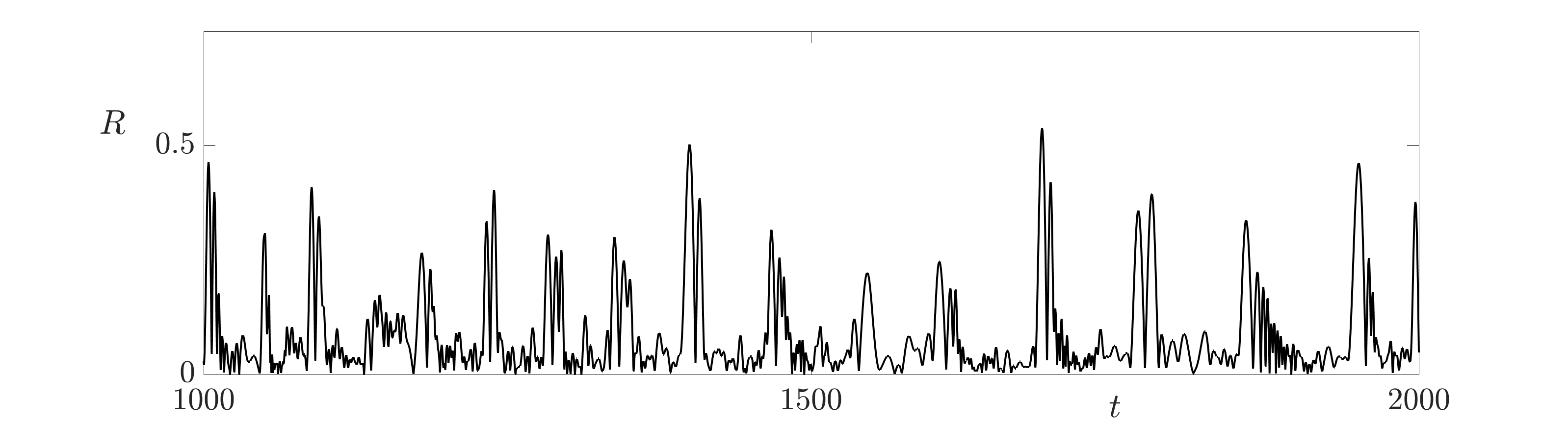
4.1 An application to the structure–function relationship in large-scale brain dynamics
The weakly-coupled-oscillator theory that we described in section 4 is natural for exploring relationships between the brain’s structural connectivity (SC) and the associated supported neural activity (i.e., its function). There are studies of the SC of the human brain, and graph-theoretic approaches have revealed a variety of features, including a small-world architecture [11], hub regions and cores [108], rich-club organization [16], a hierarchical-like modular structure [147], and cost-efficient wiring [17]. One can evaluate the emergent brain activity that SC supports using functional-connectivity (FC) network analyses [13], which describe patterns of temporal coherence between brain regions. Researchers have associated disruptions in SC network and FC networks with many psychiatric and neurological diseases [12]. A measure of FC that is especially appropriate for network models of the form eq. 47 is the pairwise phase coherence
| (50) |
Models of interacting neural masses yield natural choices of the phase-interaction function [71, 51]. For simplicity, we use a biharmonic phase-interaction function [68]
| (51) |
to illustrate how SC can influence FC. Using the results of the present section, we find that the stability boundary for the synchronous state is , which yields . Direct simulations of the phase oscillator network eq. 47 using human connectome data (parcellated into 68 brain regions) beyond the point of instability of the synchronous state reveal very rich patterns of pairwise coherence eq. 50. These complicated FC dynamics reflect the fact that all eigenmodes of the graph Laplacian are unstable, leading to network dynamics that mixes all of these states. In fig. 9, we show a plots of the emergent FC matrix from the network model eq. 47 and the interactions that are prescribed by the SC matrix.
4.2 Dead zones in networks with refractoriness
Consider once again a phase-oscillator network (47) that one obtains from a phase reduction of a weakly coupled system eq. 1 with coupling function eq. 2. The phase-interaction function has a dead zone if is an open interval on which [6]. Let denote the union of all dead zones of . When the phase difference , oscillator does not respond to changes in oscillator because the connection between them is temporarily absent. Therefore, dead zones of the interaction function lead to an effective decoupling of network nodes for certain network states . For a state , the effective interaction graph is a subgraph of the underlying structural network (which is defined by the connection strengths ) that include only the edges for which . Along solution trajectories, the effective interaction graph evolves with time. The set of subgraphs of the underlying structural network (i.e., graph) that are realizeable by trajectories of the system depends on the dead zones of the coupling function . Ashwin et al. [6] explored the interplay between dead zones of coupling functions and the realization of particular effective interaction graphs, and they began to explore how the dynamics of the associated coupled system corresponds to changing effective interactions along a trajectory.
Because one derives the phase-oscillator network eq. 47 from the original nonlinear-oscillator network described by eq. 1, eq. 2, it is natural to examine conditions on the nonlinear oscillator dynamics that yield a dead zone of the phase-interaction function . Both the coupling function and the iPRC influence whether or not there is an open interval with for all . See Ashwin et al. [7] for conditions for dead zones for relaxation oscillators with a separable coupling that acts only through one component of . Here a coupling function is separable if it can be written as
| (52) |
where is an input function and is the response function and denotes the Hadamard (element-wise) product of the vectors and . They also showed that pulsatile coupling can yield -approximate dead zones , on which .
In the present section, we show how to obtain -approximate dead zones in the phase-interaction function for networks of synaptically coupled PWL neuron models with refractoriness. Many neural oscillators have a refractory period after emitting an action potential (i.e., a nerve impulse). During this time, the neuron does not respond to input. For a phase-oscillator, during the refractory period, input does not cause the oscillator phase to advance thereby preventing further firing events. Therefore, the iPRC, is approximately for one or more intervals , where is the oscillator period. An example of a planar PWL model with such a refractory period is the continuous McKean model with “three pieces” [99, 29]. This is a PWL caricature of the FHN model, with the -nullcline broken into three pieces, which partitions the phase space into three zones, with two switching manifolds. The dynamics of the system satisfy
| (53) |
where , , and (to approximate the cubic -nullcline) is given by equation eq. 128. The dynamical system eq. 53 has a stable periodic orbit when there is a single unstable equilibrium on the center branch of the cubic -nullcline. In Figure 10, we show the phase portrait for parameter values with a stable periodic orbit. See appendix A for further details about the model.

For , the dynamics of the voltage are fast and the dynamics of the recovery variable are slow. Therefore, as , the system spends most of its time on the left and right branches of the -nullcline, with fast switching between the two branches. Consequently, (i.e., the component of the iPRC) is approximately for much of the limit cycle, with peaks corresponding to locations near the switching planes. In Figure 11, we show (and on the limit cycle) for . In the singular limit, the iPRC for this model is discontinuous [73, 28].

We now compute the phase-interaction function for a network of synaptically coupled continuous McKean neurons with time-dependent forcing:
| (54) |
Suppose that the synaptic input from neuron takes the standard “event-driven” form
| (55) |
where denotes the th firing time of neuron and the causal synaptic filter describes the shape of the post-synaptic response.
For a phase-locked system, one writes the firing times as for a phase offset . Therefore, the phase-interaction function is
| (56) |
where . Because is -periodic, we can write , where . Consequently,
| (57) |
where is the Fourier transform of the causal synaptic filter . That is, , where . If we adopt the common choice
| (58) |
where and is a Heaviside step function, then
| (59) |
In Figure 12, we show the phase-interaction function for two values of . This interaction function has two large dead zones. The larger the value of , the larger the dead zones of . For the chosen parameter values, the dead zones of are symmetric for large values of [6]. (That is, if , then . Such a coupling function is “dead-zone symmetric”.) This symmetry places restrictions on the effective interaction graphs which can be realized by the trajectories of the model. For example, if is dead-zone symmetric, then all of the effective interaction graphs for are undirected [6, Proposition 3.7]. In the limit , we also observe that is a scaled version of the component of the iPRC. This follows from and the fact that , giving pulsatile coupling.

5 Phase–amplitude networks
We now consider the second-order approximation eq. 33–eq. 34 that allows us to use both phase and amplitude coordinates to treat oscillatory network dynamics. In contrast to the phase-only approach in section 4, there has been much less work on the theory and applications of phase–amplitude networks although this is now growing, as exemplified by the work in [162]. Because of both this and to facilitate our exposition, we focus on a small network of two identical planar oscillators with linear coupling through the component. Pairs and larger networks of linearly coupled smooth Morris–Lecar neurons are considered in Nicks et al. [106] where conditions for linear stability of various phase-locked states in globally coupled phase-amplitude networks are also derived. Our discussion parallels the one in Ermentrout et al. [44] for a smooth model of synaptically coupled thalamic neurons [133].
Specifically, we consider equation eq. 1 with oscillators, a coupling strength of , and
| (60) | ||||
To determine the form of in the phase–amplitude equations eq. 33–eq. 34 to obtain the corresponding phase-amplitude reduction of the network equations eq. 1, we write and assume that the amplitudes are . Substituting this expression into eq. 33 and eq. 34 and keeping terms up to order yields the phase-amplitude reduced network equations
| (61) | ||||
where we give the detailed forms of the doubly -periodic functions in appendix E.
To further reduce the system eq. 61 to a phase-difference form, we use averaging (see section 4) and write and . This yields
| (62) | ||||
In fig. 13, we show the six interaction functions for the PWL Morris–Lecar model. We compute these functions using the Fourier representation that we described in section 4. Note that these six functions are all that is needed to describe the phase-amplitude reduced dynamics of networks of any finite size [113, 106].


For the synchronous -amplitude solution , the Jacobian of eq. 62 has the form
| (63) |
where we have used the fact that linear coupling gives and . All eigenvalues have negative real part, so the synchronous solution is linearly stable when (which we assume to obtain a stable periodic orbit), , and . Reducing to the phase-only description by taking recovers the result that the synchronous solution is linearly stable when . One can similarly determine stability conditions for the antisynchronous state (for which the phase difference between the two oscillators is ). For the antisynchronous state, the shared orbit satisfies , where , which is constant (so that the orbit coincides with an isostable of the node dynamics) [106].
Importantly, for both solutions, the phase-only reduction does not predict any bifurcations from changing , whereas the phase–amplitude approach does allow this possibility. This is the case because both the eigenvalues of eq. 63 and of the Jacobian for the antisynchronous state have a richer dependence on the coupling strength . See fig. 14 for an interesting bifurcation diagram for the PWL Morris–Lecar model that we obtain by varying . We see that we can restabilize the synchronous state by increasing when . Moreover, at smaller values of , stable periodic orbits arise from a Andronov–Hopf bifurcation of the antisynchronous state. In one region, for which , our analysis predicts that there are no stable solution branches. Direct numerical simulations (see fig. 16) of the full model eq. 127 confirm this prediction.

Although the qualitative predictions of the phase–amplitude formalism are better than those of the phase-only formalism, it remains to be seen if these predictions can also give successful quantitative insights. We explore this issue in section 6.
6 Strongly coupled oscillator networks
In previous sections, we explored how collective behavior (such as phase-locked states) arises in weakly coupled networks. We considered the dynamics of the system eq. 1 on a reduced phase space that is given by the Cartesian product of each oscillator’s phase and possibly a subset of the oscillator amplitudes. However, the assumption of weak coupling is not valid in many real-world situations. There are far fewer results for strongly coupled oscillator networks than for weakly coupled oscillator networks, and the former are often restricted to special states such as synchrony [33, Chapter 7].
One popular approach to obtain insights into the behavior of strongly coupled oscillators in the context of smooth dynamical systems is the master-stability-function (MSF) approach. The MSF approach55 5 At least on occasion, MSF approaches were used before they were invented officially in the 1990s. See Segel and Levin [137] (a conference-proceeding paper from 1976). of Pecora and Carroll [117] to assess the stability of synchronous states of a network in terms of the spectral properties of the network’s adjacency matrix is exact. It does not rely on any approximations, aside from those in numerical implementations (to construct periodic orbits and compute Floquet exponents). In the present section, we describe how to augment this MSF approach for PWL systems using the saltation operators that we described in section 2.1. For PWL systems, one can use semi-analytical approaches (with numerical computations only for times of flight between switching manifolds) instead of the numerical computations (i.e., simulations of differential equations) that one uses for smooth nonlinear systems.66 6 Recently, Corragio et al. [34] used an alternative approach for systems with a so-called “-QUAD property” (which includes many discontinuous neural, genetic, and impact networks) to prove global asymptotic convergence to synchronization in networks of piecewise-smooth dynamical systems.
6.1 The master stability function for nonsmooth systems
To introduce the MSF formalism, we start with an arbitrary connected network of coupled identical oscillators eq. 1, eq. 2 with . The output for each oscillator is determined by a vector function (which can be either linear or nonlinear). The network dynamics are
| (64) |
where, the matrix , with entries , is the graph Laplacian eq. 49. By construction, the matrix has row sums. The constraints define the invariant synchronization manifold, where is a solution in of the associated uncoupled system. That is, . Any motion that begins on the synchronization manifold remains there, so the associated synchronized state is flow-invariant.
When all oscillators are initially on the synchronization manifold with identical initial conditions, they always remain synchronized. To assess the stability of a synchronized state, we perform a linear stability analysis by inserting a perturbed solution into eq. 64 to obtain the variational equation
| (65) |
where and , respectively, denote the Jacobians of and , which one evaluates at the synchronous solution . We introduce and use the tensor product (i.e., Kronecker product) for matrices to write the variational equation as
| (66) |
We organize the normalized right eigenvectors of into a matrix such that , with , where (with ) are the corresponding eigenvalues of . We introduce a new variable using the linear transformation to obtain a block-diagonal system
| (67) |
where is the identity matrix. This yields a set of decoupled -dimensional equations,
| (68) |
that are parametrized by the eigenvalues of the graph Laplacian . The Jacobians and are independent of the block label . Because the row sums of are , there is always a eigenvalue , with a corresponding eigenvector that characterizes a perturbation that is tangential to the synchronization manifold. The remaining transversal perturbations (which are associated with the other solutions of equation eq. 68) must damp out for the synchronous state to be linearly stable. In general, some eigenvalues of may be complex. (For example, this can occur when the adjacency matrix is not symmetric.) This leads us to consider the system
| (69) |
All of the individual variational equations in the system eq. 68 have the same structure as that of the system eq. 69. The only difference is that . Equation eq. 69 is the so-called master variational equation. To determine its stability, we calculate its largest Floquet exponent [65] as a function of . The resulting function is the so-called master stability function (MSF). More explicitly, for a given the MSF is the function that maps the complex number to the largest Floquet exponent of the dynamical system eq. 69. The synchronized state of a network of coupled oscillators is linearly stable if the MSF is negative at , where ranges over all eigenvalues of the matrix except for .
The Laplacian form of the coupling in equation eq. 64 guarantees that there exists a synchronous state. However, other forms of coupling are also natural. For example, consider
| (70) |
Substituting , with }, into equation eq. 70 yields
| (71) |
To guarantee that all oscillators have the same behavior, we assume that for all . If the constant is , then we say that the system is balanced [39, 156, 134, 132]. In a balanced network, the existence of a synchronous network state is independent of the interaction parameters, so varying these parameters cannot induce any nonsmooth bifurcations (arising from a change of the orbit shape and its possible tangential intersection with a switching manifold).
One can apply the MSF framework to chaotic systems, for which one calculates Liapunov exponents instead of Floquet exponents [119, 117, 37]. One can also generalize the MSF formalism to network settings in which the coupling between oscillators includes a time delay [86, 38]. A synchronous solution is a very special network state, and more elaborate types of behavior can occur. An example is a “chimera state”(see [31, 94]), in which some oscillators are synchronized but others behave asynchronously [111]. The original MSF approach allows one to investigate the stability of networks of identical oscillators, but it has been extended to study stability in networks of almost identical oscillators [148]. For other discussions of the MSF formalism and its applications, see [8, 4, 118, 127].
One cannot directly apply the MSF methodology to networks of nonsmooth oscillators, and it is desirable to extend it to such systems. We first review a technique that adapts the MSF to PWL systems [31], and we then apply this approach to the models in section 2. We seek to show how the linear stability of the synchronous solution changes under variations of the coupling strength in networks of coupled oscillators.
For networks of the form eq. 64 with linear vector functions (including the “linear diffusive case” ) that one builds from PWL systems of the form eq. 3, both and are piecewise-constant matrices. Therefore, in each region , equation eq. 69 takes the form
| (72) |
where and . We solve eq. 72 using matrix exponentials. This yields , where is given by equation eq. 7, although we need to be careful when evolving perturbations through the switching manifolds. Using the notation , at each event time , we write . We then use the transformation and obtain , which has dimensions and an block structure. The action of the saltation operator on each block is . We use the technique in appendix B to treat perturbations across a switching boundary. After one period of motion (with switching events), this yields , where
| (73) |
and (see eq. 17). For PWL systems, all of the individual variational equations, which take the form eq. 68, have the same structure as that of the system eq. 72. The only difference is that now there is an additional term . Therefore, by choosing a reasonable value of in the complex plane, we can determine the stability of eq. 68 by checking that the MSF of eq. 72 is negative for each . Alternatively, we can calculate for each ; we use the notation to emphasize this. We then obtain that the synchronous state is linearly stable if the periodic solution of a single oscillator is linearly stable and the eigenvalues of , for each lie within the unit disc.
The power of the MSF approach is that it allows one to treat the stability of synchronous states for all possible networks. One first computes the MSF and then uses the spectrum of the chosen network to determine stability. Unlike in weakly-coupled-oscillator theory, one can perform the MSF stability analysis without making any approximations.
6.2 MSF versus weakly-coupled-oscillator theory for systems of oscillators
Before we present applications of the augmented MSF to a few example nonsmooth systems, we compare and contrast this exact approach to results from weakly-coupled-oscillator theory without focusing too much on network structure. Consider a simple reciprocal network (i.e., all coupling is bidirectional) of two nodes with an interaction that is described by eq. 60. The nonzero eigenvalue of the graph Laplacian of this network is . For the phase-only description, the synchronous state is linearly stable if (see section 4). For the phase–amplitude description, the synchronous state is linearly stable if the three eigenvalues of eq. 63 are all in the left-hand side of the complex plane (see section 5). For the exact approach of the present section, the synchronous state is linearly stable if the MSF is negative at (see section 6.1). Using the same oscillator parameters as those in fig. 1 and fig. 2, we find that weakly-coupled-oscillator theory sometimes fails to capture the behavior that is predicted by the exact (MSF) approach. For the McKean and absolute models, all three approaches give the same qualitative prediction that the synchronous state is linearly stable for small positive (i.e., for weak coupling) and this stability persists for larger (i.e., strong coupling).

For the PWL Morris–Lecar model (see eq. 127), the prediction from the phase-only approximation is that synchrony is always unstable for weak positive coupling. By contrast, the phase–amplitude approximation and MSF approach predict that synchrony can restabilize with increasing coupling strength , although they predict somewhat different values for the critical coupling strength at which the network restabilizes. In Figure 15, we plot the real part (where ) of the largest Floquet exponent from the MSF as a function of . In the same figure, we plot the the real part of the largest eigenvalue from the phase–amplitude approximation. The phase–amplitude prediction is that , whereas the (exact) MSF prediction is that . The phase-only theory is incorrect qualitatively, the phase–amplitude theory is correct qualitatively, and the MSF approach (which agrees with direct numerical simulations) is correct both qualitatively and quantitatively. In fig. 14, we explored the behavior of the PWL Morris–Lecar model in the phase–amplitude reduction for coupling strengths (where synchrony is unstable) using bifurcation analysis, which predicts the existence of a stable antisynchronous state (for which there is a relative phase of between the two oscillators) and of frequency-locked states (i.e., states in which oscillators are synchronized at the same frequency) of different amplitudes. Direct numerical simulations (see fig. 16) confirm these predictions.


For the PWL homoclinic model, both the phase-only approximation and the phase–amplitude approximation predict that synchrony is always unstable for weak positive coupling in a two-oscillator reciprocal network. These predictions are both inconsistent with the MSF prediction (which agrees with direct numerical simulations) of two windows of positive coupling with stable synchronous states. In Figure 17, we show a plot of the MSF that reveals a nontrivial structure, with two ellipsoidal regions where it is negative. (There is a very small ellipsoidal region near the origin that is not visible with the employed scales.) We also show a slice through along the real axis that illustrates where the real part of the largest network Floquet exponent is negative, generating two regions in which the synchronous state is stable.


6.3 A brief note about graph spectra
As we have seen in our discussions, the spectrum of a graph is important for determining the stability of the synchronous state in both the weakly-coupled-oscillator and MSF approaches. We thus briefly discuss the spectra of a few simple but notable types of graphs. See [155] for a thorough exploration of graph spectra.
For a network (i.e., a graph) of nodes, one specifies the connectivity pattern by a coupling matrix (which is often called an “adjacency matrix”) with entries . The spectrum of the graph is the set of eigenvalues of the matrix . This spectrum also determines the eigenvalues of the associated combinatorial graph Laplacian . In our discussion, we denote the eigenvalues of by , with , and we denote the corresponding right eigenvectors by .
- Global.
-
The simplest type of network with global coupling has adjacency-matrix entries . The associated network is fully connected with homogeneous coupling. The matrix has an eigenvector with eigenvalue and degenerate eigenvalues , for , with corresponding eigenvectors that satisfy the constraint .
- Star.
-
A star network has a hub-and-spoke structure, with a central oscillator that is adjacent to leaf nodes (which are not adjacent to each other). Star networks arise in computer-network topologies in which one central computer acts as a conduit to transmit messages (providing a common connection point for all nodes through a hub). This star-graph architecture has the adjacency matrix
(74) for some constant . If , the matrix has an eigenvalue with corresponding eigenvector , an eigenvalue with corresponding eigenvector , and degenerate eigenvalues , for , with corresponding eigenvectors of the form that satisfy the constraint .
- Circulant.
-
A circulant network’s adjacency matrix has entries . Its rows are shifted versions of the column vector . Its eigenvalues are , where is an th root of unity. The eigenvectors are .
6.4 Network symmetries and cluster states
Perfect global synchronization is just one of many states that can emerge in networks of oscillators. Indeed, one expects instabilities of the synchronous state to generically yield “cluster states”, in which subpopulations synchronize, but not necessarily with each other. Such cluster synchronization has been relatively well-explored in phase-oscillator networks [9, 22], although less is known about it in networks of limit-cycle oscillators. For this more general scenario, researchers have made progress in networks with symmetry or when the coupling has a linear diffusive (i.e., Laplacian) form [58, 60, 123, 124, 15].
Pecora et al. [120] and Sorrentino et al. [146] extended the MSF approach (see section 6.1) to analyze the stability of cluster states that stem either from network symmetries or from Laplacian coupling (see equations eq. 64 and eq. 70). Cluster states arise naturally in networks with symmetry, and cluster synchronization can also occur in networks without symmetry when some of the nodes have synchronous input patterns [61]. For networks of identical oscillators that satisfy equation eq. 64, a symmetry of the network is a permutation of the nodes that does not change the governing equations. These permutations are precisely the ones that satisfy , where is the graph Laplacian eq. 49 and is the permutation matrix for the permutation . The network symmetries form a group that is isomorphic to the group of automorphisms of the graph that underlies the network.
For a given adjacency matrix, one can identify the automorphism group using computational-algebra routines (such as those that are implemented in SageMath [152]). One can then apply the algorithms in [146] to enumerate all possible cluster states for the associated network structure. Some of these correspond to isotropy subgroups77 7 A subgroup of a Lie group is an isotropy subgroup for the action of on a vector space if it is the largest subgroup that leaves invariant some vector in [58, 59]. and thus arise from network symmetries. The orbit under of node is the set . The orbits permute subsets of nodes among each other and thereby partition the nodes into clusters. Nodes that are part of the same orbit (i.e., in the same cluster) have synchronized dynamics for any (see [61, Thm III.2]). Isotropy subgroups that are conjugate in lead to cluster states with identical existence and stability criteria [59, 8]. The remaining possible cluster states arise from the specific choice of Laplacian coupling. One can determine them using an algorithm that considers whether or not merging two clusters in a state that is determined by symmetry yields a dynamically valid state (i.e., whether or not it yields consistent equations of motion when is the same for all nodes in the merged cluster). Sorrentino et al. [146] referred to such cluster states as “Laplacian clusters”. See [146] for a detailed explanation of the algorithm to determine these clusters, and see [107] for an illustration of this algorithm. One can automate this algorithm using computer-algebra tools [152].
The above steps yield a list of possible cluster states. The existence and stability of these states depends on the node dynamics , the output function , and the coupling strength . The presence of symmetry in a system imposes constraints on the form of the Jacobian matrix, which one can use to greatly simplify stability calculations. For periodic cluster states that one predicts from symmetry, there are well-established methods for stability calculations in symmetric systems to block-diagonalize the Jacobian and generalize the MSF formalism [59, 58]. Sorrentino et al. [146] extended these techniques to Laplacian cluster states. We follow [146, 107] and summarize this analysis.
Consider a periodic cluster state that arises from a network symmetry with the corresponding isotropy subgroup . The fixed-point subspace of is , which is the synchrony subspace of the cluster state. The cluster state consists of clusters , with , where . Let denote the synchronized state of nodes in cluster and recall the notation of section 6.1. The variational equation of eq. 64 about the cluster state is
| (75) |
where is the diagonal matrix with entries if and otherwise. To determine the stability of the periodic cluster state, we need to compute the Floquet exponents of equation eq. 75. We block-diagonalize the variational equation eq. 75 using the system’s symmetries to simplify this task. One can decompose the action of on the phase space into a collection of irreducible representations of (i.e., the most trivial invariant subspaces under the action of ). Some of these subspaces are isomorphic to each other; we combine these subspaces to obtain “isotypic components” [59, 58]. Each isotypic component is invariant under the variational equation (75), so one can determine the Floquet exponents by considering the restriction of this equation to each isotypic component. Therefore, the decomposition puts the variational equations into block-diagonal form. We then compute Floquet exponents for each block to determine the stability of the cluster state. See [59] for a detailed discussion of the process of isotypic decomposition and its use in stability computations. Pecora et al. [120] presented an explicit algorithm to (1) determine the isotypic decomposition for a given cluster state from symmetry and (2) compute a transformation matrix so that is block diagonal. Applying this transformation to the variational equation (75) yields a block-diagonal system of equations:
| (76) |
where and . The isotypic component of the trivial representation is , which is the synchronization manifold. This gives an block in that corresponds to perturbations within the synchronization manifold; one of the Floquet exponents will be and the remaining correspond to intercluster perturbations. The remaining blocks correspond to the isotypic components of other irreducible representations of . When the node-space representation has isomorphic copies of a particular irreducible representation, we obtain a block of size . Such a block corresponds to a perturbation that is transverse to the synchronization manifold (intracluster perturbations); the associated Floquet multipliers determine the stability under a synchrony-breaking perturbation. For a cluster state to be linearly stable, all Floquet exponents (except the one that is always ) must have a negative real part.
For a periodic Laplacian cluster state, the synchronization manifold is an invariant subspace, but it is not the fixed-point subspace of any subgroup of . However, we can still block-diagonalize the Laplacian so that the top-left block corresponds to perturbations within the synchronization manifold. To do this, we use the algorithm of Sorrentino et al. [146]. Suppose that we start with a cluster state from symmetry with isotropy group that has clusters and a variational equation that is block-diagonalized by the matrix . Suppose that we merge two clusters in this state to obtain a Laplacian cluster state. Upon this merger, the dimension of the synchronization manifold decreases by and the dimension of the transverse manifold increases by . We obtain new coordinates on the synchronization manifold by transforming the new synchronization vector in the node-set coordinates (this vector has entries in the position of each node in the new merged cluster and entries everywhere else) into the coordinates of the block-diagonalization of the cluster state with isotropy group . The orthogonal complement of the new synchronization vector gives the new transverse direction. We normalize the resulting vectors and use them as rows of an orthogonal matrix whose other rows satisfy . The matrix block-diagonalizes to a matrix that has a top-left block of size . Therefore, the transformation matrix block-diagonalizes the variational equation for the Laplacian cluster state, facilitating the ability to determine both the Floquet exponents within the synchronization manifold and the transverse Floquet exponents. This process for computing the required matrix is illustrated with examples in [146] and [107].
For PWL systems of the form eq. 64 with linear vector function , it is relatively straightforward to construct the periodic orbits for a cluster state and to determine its stability by applying the modified Floquet theory (which accounts for the lack of smoothness of the dynamics) of section 2.1 to the block-diagonalized system. For example, suppose that we have a small network of linearly coupled oscillators whose dynamics satisfy the absolute PWL model (see fig. 1(a)). As an illustration, consider the five-node network in [146] with graph Laplacian matrix
| (77) |
The network supports a Laplacian cluster state with clusters and [146, 107]. For this cluster state, and , where for and the invariant-subspace equations have the form , where and
| (78) |
and we define , , , and in table 1. Also let so that the coupling acts only through the first component. This is a -dimensional PWL system with two switching planes, and . One can construct the periodic orbit on the -dimensional synchronous manifold by following the method that we outlined in section 2. Starting from the initial data , we now have to solve a system of seven nonlinear algebraic equations for , , and and the four switching times , , , and (see fig. 18).

With the block-diagonalization of the variational equation (76), one uses the initial data and switching times to explicitly compute the Floquet multipliers of the periodic orbit. One can compute Floquet multipliers that correspond to perturbations within the synchronization manifold without using the block-diagonalization. We have
| (79) |
which one can solve using matrix exponentials, being careful to use saltation matrices to evolve perturbations through switching manifolds. After one period, , where is the monodromy matrix on the synchronization manifold. Considering all evolutions and transitions through switching manifolds, we obtain
| (80) |
with saltation matrices
| (81) | ||||
| (82) |
The Floquet multipliers for perturbations within the synchronization manifold are the eigenvalues of the monodromy matrix . One of these eigenvalues is always , corresponding to perturbations along the periodic orbit.
The block-diagonalization of for the cluster state that we have been discussing is [146, 107]
| (83) |
In the directions that are transverse to the synchronization manifold, this block-diagonalisation yields the following three decoupled Floquet problems:
| (84) | ||||
which (as usual) one can solve using matrix exponentials and saltation matrices. This yields , where the monodromy matrices for the transverse directions are
| (85) | ||||
and
| (86) |
The eigenvalues of the mondromy matrices , with give the Floquet multipliers for directions that are transverse to the synchronization manifold.
The change of basis from coordinates to coordinates has no effect on the action of the saltation matrices. (Recall that .) To evolve through a discontinuity, we write , where
| (87) |
Therefore, , where
| (88) |
Because the vector field of the absolute model is continuous, all saltation matrices are the identity matrix. One then does an algebraic calculation to show that the cluster state is stable for the choice of parameters in fig. 1(a). One finds bifurcations of the periodic orbit by determining when the Floquet multipliers leave the unit disk. As one varies the parameters, the order of the times at which trajectories cross the switching planes can also change. One constructs bifurcation diagrams by similarly treating all types of cluster states from network symmetries and Laplacian clustering.
For the absolute model with the choice of parameters in fig. 1(a) and interaction function , we show the bifurcations from varying the coupling strength in fig. 19. All of the bifurcations from stable states are tangent bifurcations [84], in which a Floquet multiplier passes through the value .

One can use the above approach to determine the stability of cluster states in any network of PWL nodes; see [107] for more examples. The computational difficulty of applying the MSF approach for a cluster state scales with the number of clusters in the state and with the number of switching planes in the PWL model of the individual oscillators. It does not scale with the size (i.e., the number of nodes) of a network. Finally, we note that one can view synchrony as a single-cluster state, for which the above methodology reduces to the standard MSF approach in section 6.1.
6.5 An application to synaptically coupled, spiking neural networks
It is common to model spiking neural networks using integrate-and-fire (IF) neurons. Coombes et al. [32] explored the nonsmooth nature of systems of IF neurons. The MSF approach has been used to study synaptically coupled networks of nonlinear (specifically, adaptive exponential) IF neurons [87], for which one uses numerical computations to obtain periodic orbits. Nicks et al. [107] showed how to make analytical progress on the dynamics of PWL planar IF neurons.
We follow Nicks et al. [107] and consider a network of synaptically coupled planar IF neurons with the time-dependent forcing . The synaptic input from neuron takes the standard event-driven form eq. 55 We adopt the common choice of a continuous -function, so that is eq. 58. We can then express as the solution to the impulsively forced linear system
| (89) |
We exploit the linearity of the synaptic dynamics between firing events to write the network model in the form eq. 70 with , where and has the form eq. 3, with
| (90) |
and , and one applies the jump operator whenever . The vector function that specifies the interaction is .
For a synchronous orbit of the type in fig. 1(d) (so that a trajectory only visits the region of phase space that is described by and the -periodic trajectory satisfies the constraints , , , and ), we only need to consider saltation at firing events and the saltation matrix takes the explicit form
| (91) |
See appendix B for the general formula for the saltation operator of a PWL system. In this case, the expression for in eq. 73 reduces to
| (92) |
where and is the th eigenvalue of . The matrix is a constant matrix with entries if and and otherwise. Therefore, using equation eq. 92 and the prescription in section 6.1, we are able to construct MSF (see fig. 20).

As a particular realization of a network architecture that guarantees synchrony, we use a balanced ring network with odd and . We calculate the distances modulo and use the decay rate . We choose the parameter so that (a balance condition) for the network size and a scale . The eigenvalues of the associated (symmetric and circulant) adjacency matrix are real and given by . The balance condition enforces . Additionally, for , so any excited pattern (which arises from an instability) is given by a combination for some . Given the shape of the MSF function in fig. 20, one determines the value of using . In fig. 21, we compare direct simulations of a network versus the predictions of the MSF. When the network’s eigenvalues lie within the region where the MSF is negative, small perturbations of synchronous initial data decay away and the system settles to a synchronous periodic orbit, as expected. When one of the eigenvalues crosses the level set of the MSF from negative to positive, two types of instabilities emerge. One of them leads to a spatiotemporal pattern of spike doublets (i.e., a burst of two spikes), which arise because an eigenvalue of leaves the unit disk at (through a period-doubling bifurcation), and the other yields a periodic traveling wave (with asynchronous firing) because an eigenvalue of leaves the unit disk at (through a tangent bifurcation).
6.6 An application to neural-mass networks
The human brain has roughly neurons and roughly synapses. Although there is general consensus that the synaptic interactions between neurons drive brain dynamics, these astronomical numbers prohibit the construction, analysis, and simulation of an entire brain network that is built from single-neuron models such as the absolute model or the Morris–Lecar model (see section 2). Instead, it is instructive to coarse-grain neural behavior by grouping neurons and studying the interactions between these groups. This idea led to neural-mass models [8], which describe the average dynamics of large populations of neurons.
One of the most influential neural-mass models is the Wilson–Cowan model [166, 165]
| (93) |
where and , respectively, indicate the activity of excitatory and inhibitory populations of neurons. A firing-rate function , which researchers often take to have a sigmoidal shape, mediates the interactions between the two populations. The quantities represent background inputs, and (with ) denote connection strengths between populations. The positive constant encodes the relative time scale between the dynamics of the two populations.
To make analytical progress, Coombes et al.[30] considered a PWL firing-rate function of the form
| (94) |
With this choice, it is straightforward to compute periodic orbits of the dynamical system (93) and to determine their linear stability using the techniques that we described in section 2. One can think of the system (93) as modeling an appropriately chosen brain region, so coupling oscillators that satisfy (93) lets one investigate the dynamics of interacting brain regions. By introducing the coupling matrices , with , we obtain a network of interacting oscillators with dynamics
| (95) | ||||
| (96) |
Although the dynamical system eq. 96 is not exactly in the form that we described in section 6.1, one can analyze this network using essentially the same MSF techniques. For simplicity and to guarantee the existence of a synchronous network state, we impose the row-sum constraint for . These row-sum constraints are natural for networks arranged on a ring, because the coupling matrix is circulant (see section 6.3). The synchronous network state satisfies for all , where satisfies equations eq. 93.
It is convenient to introduce the vector and change variables by writing , where
| (97) |
the matrix , and is an -dimensional vector with all entries equal to . One can then succinctly describe the switching manifolds by the relations and , and the dynamics takes the form
| (98) |
where . We denote the synchronous solution by , , with
| (99) |
and consider small perturbations such that . We thereby obtain
| (100) |
where is the Jacobian of evaluated along the periodic orbit.
As we showed in section 6.1, we need appropriately diagonalize (100). Suppose that we can diagonalize all with respect to the same basis, and let be the matrix whose columns consist of the basis vectors. Such simultaneous diagonalization is feasible for circulant matrices, which naturally obey the above row-sum constraint. Let , with , denote the eigenvalues of . We then write
| (101) |
where
| (102) |
Additionally, .
Consider perturbations of the form . Equation eq. 100 then implies that the linearized dynamics satisfies
| (103) |
where is the Jacobian of . The matrix is a piecewise-constant matrix that is nonzero only if either or . Analogously to eq. 68, equation eq. 103 has a block structure in which the dynamics in each of blocks satisfies
| (104) |
with .
The problem that is defined by eq. 104 is time-independent between switching manifolds, so one can construct a solution in a piecewise fashion from matrix exponentials and write . One can then construct a perturbed trajectory over one period of oscillation in the form , where is
| (105) |
with
| (106) |
Note (and see equation eq. 73) that there is no saltation (i.e., ).
As an illustration, consider a network of Wilson–Cowan oscillators on a ring graph with an odd number of nodes. Let be the distance between nodes and . We then define a set of exponentially decaying connectivity matrices
| (107) |
In this example, are four circulant matrices; they are parametrized by the four quantities , which respect the row-sum constraints . In Figure 22, we plot the eigenvalues of for for two different parameter choices. In fig. 22(a), all of the eigenvalues (excluding the one at that arises from time-translation invariance) lie within the unit disk. In fig. 22(b), one eigenvalue leaves the unit disk along the negative real axis. This latter scenario predicts an instability of the synchronous state. In the inset of panel (b), we show the eigenvector that corresponds to the eigenvalue that crosses to the outside of the unit disk. The prediction of this instability is in excellent agreement with direct numerical simulations [30].


6.7 An application to cardiac alternans
One can conceptualize a beating heart as a network of muscle cells in which each heartbeat results from their coordinated contraction and subsequent relaxation. Because the dynamics of an organ results from the orchestrated behavior of individual cells, a major avenue in cardiac research is the investigation of the dynamical repertoire of individual cardiac muscle cells [129]. Molecular changes at the individual-cell level can yield irregular cell behavior, which then feeds forward to pathological heart dynamics (such as cardiac arrhythmias). A vital component that determines the behavior of cardiac muscle cells is the intracellular calcium () concentration. In basic terms, rises and falls of the cytosolic concentration are responsible for muscle contraction, and irregularities and abnormalities of the intracellular dynamics have been linked to a plethora of cardiac pathologies [90].
The intracellular concentration in cardiac muscle cells has rich spatiotemporal patterns that arise from the interplay of diffusively coupled calcium-release units (CRUs). One can decompose each CRU into compartments with fluxes between them, so a cardiac muscle cell corresponds to a network of networks. In other words, each node of the cellular network is itself a network (i.e., a CRU). Using a 5-dimensional PWL representation of a well-established cardiac model [153], one can express the dynamics of a network of CRUs as
| (108) |
where is a -dimensional vector. Each entry , with }, is the 5-dimensional state vector of a single CRU. The matrix is constant and block diagonal with entries in the set . The constant matrices are associated with a single CRU, analogously to the matrices and in equation eq. 3. As usual, the matrix denotes the combinatorial graph Laplacian matrix of the network and the matrix encodes which variables are coupled and how strongly they are coupled. The time-dependence distinguishes the present example from the other examples in this section. The explicit time-dependent drive , which is -periodic, models an experimental condition that is known as a voltage clamp, which is used often to disentangle the different cellular mechanisms that contribute to the complex spatiotemporal patterns of the intracellular concentration of cardiac cells.
Because of the explicit time-dependence in equation eq. 108, the switching manifolds are not only state-dependent (as in all of the previous examples in this section), but some of them are also time-dependent. This leads to a system in which any trajectory is determined by a sequence of state-dependent and time-dependent switches [153, 88, 157]. As demonstrated in section 2, one can readily compute the synchronous network state of eq. 108 using matrix exponentials. One can then linearize equation eq. 108 around the synchronous network state by using the ansatz and following the general approach in section 6. Analogously to equation eq. 68, this yields
| (109) |
where and are the eigenvalues of . Because we are perturbing from the synchronous network state, we assume that all CRUs have the same associated to obtain eq. 109.
The dynamical system eq. 109 is continuous at the switching manifolds, so one can obtain its solution using matrix exponentials. Let denote the time-of-flight for when the dynamics are associated with , let denote the period of the synchronous state, and let denote an initial perturbation. According to the relation eq. 73 and noting that there is no saltation (i.e., ), the perturbation after one period is , where
| (110) |
As we showed in section 6.1, one can use the relation eq. 110 to construct the MSF. In Figure 23, we illustrate that the topology of the MSF can vary substantially across different coupling regimes. In the left panel of fig. 23, the zero contour of the MSF forms a closed loop; the MSF is negative inside the loop and positive outside it. On the contrary, in the right panel of fig. 23, there are two distinct regions in which the MSF is negative. The colors reveal that if the MSF changes sign along the real axis, then the only instabilities are either a period-doubling bifurcation (i.e., a bifurcation) or a tangent bifurcation (i.e., a bifurcation).


As was demonstrated by Lai et al. [88], MSF plots like those in fig. 23 allow one to understand abrupt changes in spatial patterns from small changes of a single parameter. In Figure 24, we illustrate the behavior that emerges when the synchronous solution destabilizes via a period-doubling bifurcation or a tangent bifurcation. In Figure 24(a), we show the peak concentration during one period of the -periodic drive for a period-doubling bifurcation. The CRUs are arranged on a regular two-dimensional grid, so one can reference each CRU by a row and column index. Each small rectangle represents the concentration of a single CRU. One can clearly see a spatially alternating pattern, which is more pronounced near the center of the figure than it is near the edges. This spatially alternating pattern also alternates in time: when a CRU has a large peak during one pacing period, it has a small peak during the next pacing period (and vice versa). In other words, each CRU exhibits a period-2 orbit and adjacent CRUs oscillate out of phase with each other. This phenomenon is known as “subcellular alternans” and is a precursor to severe cardiac arrhythmia. For the behavior in fig. 24(a), only one eigenvalue lies outside the unit disk. In fig. 24(b), we show the corresponding right eigenvector, which is in excellent agreement with direct numerical simulations. When an eigenvalue leaves the unit disk along the positive real axis, one observes a pattern like the one in fig. 24(c). As with the period-doubling bifurcation, the peak concentrations exhibit an alternating spatial pattern. However, in contrast to the period-doubling bifurcation, each CRU follows a period-1 orbit, so the peak amplitude is the same across pacing periods, rather than alternating from one pacing period to the next. In Figure 24(d), we show the eigenvector that is associated with the only eigenvalue that lies outside the unit disk for the behavior in fig. 24(b). This eigenvector also agrees excellently with direct numerical simulations.

6.8 An application to Franklin-bell networks
Benjamin Franklin was one of the leading political figures of his time, and he was also a prolific inventor and scientist. To facilitate his studies into the nature of electricity, he employed lightning as an electrical power source. To be notified when an iron rod outside his house was sufficiently electrified by lighting, Franklin employed what is now known as a “Franklin bell” [52]. A Franklin bell is a metal ball that oscillates between two metal plates, which are driven by electrical charge. A Franklin bell is an example of an impacting system; the ball velocity changes nonsmoothly when it contacts either plate. A network of Franklin bells satisfies the dynamical system [140, 136]
| (111) | ||||
| (112) |
where denotes the position of the ball of the th Franklin bell, which is restricted between two impacting manifolds at . One implicitly determines the time of the th impacting event of the th oscillator using the relation . The parameter is a global coupling strength, and the network structure is encoded by a matrix with elements . The constant is the coefficient of restitution upon impact, is a constant force (which is determined by a sum of the repelling and attracting electrostatic forces), is a damping coefficient, and sets the natural frequency of the pendulum.
It is convenient to write the dynamical system eq. 111, eq. 112 as a system of first-order differential equations (i.e., in the standard form of a dynamical system) by introducing the state vector , where . This yields
| (113) | ||||
| (114) |
The vector field is , where
| (115) |
The function is . The form of the coupling in equation eq. 113 ensures the existence of the synchronous network state . To determine its linear stability, we rewrite eq. 113 using the graph Laplacian (see section 6.1). The dynamics between impacts is
| (116) |
which has the form eq. 64. Consequently, after diagonalization, the Floquet problem for the linear stability of the synchronous network state becomes (with ), where
| (117) |
and the saltation operator is
| (118) |
As we showed in section 6.1, we obtain the MSF from eq. 117 with the replacement . In Figure 25, we illustrate the dynamics of a network of 15 Franklin bells when the adjacency matrix has entries
| (119) |
for . The MSF (see fig. 25(a)) is negative for only one , so the synchronous state is unstable. In fig. 25(b), we show the eigenvector that corresponds to the critical value . We see in fig. 25(c) that we obtain excellent agreement with direct numerical simulations. Because the adjacency matrix with the entries eq. 119 is symmetric, all of the eigenvalues are real, so is real. See Şayli et al. for a discussion of the predictive power of the MSF for an example with complex eigenvalues.


6.9 An application to coordination in cow herds
Grazing animals, such as cows, protect themselves from predators by living in herds [100], and synchronizing their behavior (by tending to eat and lie down at the same time) helps them remain together as a herd [131]. Sun et al. [149] developed a piecewise-linear dynamical system as a simplistic model to study collective in herds of cattle. One can treat some aspects of their model — both for a single cow and for a network of cows — using the focal techniques of the present paper.
Cows are ruminants. They eat plant food, swallow, and regurgitate it at some later stage; they then again chew the partly digested plant food. During the first stage (standing/feeding), they stand up to graze. However, they typically lie down and ruminate (i.e., chew the cud) in a second stage (lying/ruminating). A cow thus oscillates between two stages. One can construct a simplistic caricature of a cow by separately considering its observable state (eating, lying down, or standing) and its unobservable level of hunger or desire to lie down. Sun et al. formulated a model in terms of a variable , where with a parameter and an observable state . The variables and , respectively, represent the extent of the desire of a cow to eat and lie down. The variable represents the state of a cow, which can be eating (), lying down (), or standing (). The dynamics in the plane is confined to a box, and a cow switches between states whenever a trajectory intersects with the edge of the box.
The dynamics of takes the simple form , where
| (120) |
with hunger parameters and lying parameters . The parameter represents the rate of increase of hunger, represents the decay rate of hunger, represents the rate of increase of the desire to lie down, and represents the decay rate of the desire to lie down. One prescribes switching conditions (at the four edges of the box) using four indicator functions: , , , and . The model’s four state-transition rules take the form , where , , and . If a trajectory intersects the corner of the box, one can apply a state-tiebreaker rule [149], although we will not consider such scenarios.
The general prescription in eq. 15 yields saltation matrices at each of the four possible state transitions. They take the explicit forms
| (121) |
For a given state, one readily obtains phase-space trajectories as convex curves , with . The associated time evolution is for . Many periodic orbits are possible, and one can catalog them in terms of state-transition sequences. Sun et al. [149] identified four low-period orbits, which have the following cyclic state-transition sequences: (a) , (b) , (c) , and (d) . For example, consider a periodic orbit of type (b). Starting from , we obtain the time-of-flight from the relation . This, in turn, allows one to determine the initial data for the next piece of the trajectory. It is , from which we obtain the time-of-flight . The third and final piece of the orbit has initial data and a time-of-flight of . To determine the value of , one enforces the periodicity condition , where is the period of the periodic orbit. One thus obtains
| (122) |
To ensure that , , and , the trajectory needs to satisfy the inequality and it also needs to satisfy when . In fig. 26, we show an example of an orbit that one constructs in this fashion.

To determine the stability of this orbit, we calculate the Floquet exponent eq. 18 and obtain
| (123) |
where we use the fact that . Therefore, the orbit (if it exists) is linearly stable for . The Floquet multiplier is , so one can lose stability only through a period-doubling instability.
To model a herd (i.e., a network) of identical cows, we suppose that each cow has an associated variable that evolves according to
| (124) |
where is the indicator function
| (125) |
For , this network model describes the case that a cow feels hungrier when it notices other cows eating and feels a greater desire to lie down when it notices other cows lying down. Because the indicator functions change with time, the network has a time-dependent coupling, so one cannot use our previous MSF for it. Nonetheless, the PWL nature of the dynamics allows one to obtain analytical insights into the model’s behavior. Assuming the row-sum normalization for all , a synchronous orbit (if it exists) satisfies the equation for all , where and . Therefore, one can use the approach that we described above for a single cow to construct a synchronous orbit under the replacement . For perturbations that do not change the order (i.e., the total number of states, including repetitions) in a state-transition sequence, linearization around the synchronous state leads to the evolution of the network perturbation over one period of the form , where
| (126) |
with and . Therefore, the synchronous state is linearly stable if all of the eigenvalues of lie within the unit disk.
The above analysis allows one to generate a quantitative answer to the following question: Can herd interactions promote synchrony? Consider the choice , so that an isolated cow (i.e., ) cannot achieve a stable cycle. One can numerically calculate the eigenvalues of eq. 126 to determine whether or not there is a critical value of that brings all of the eigenvalues back inside the unit disk. Numerical calculations for several types of row-normalized networks (e.g., star networks and nearest-neighbor circulant networks) suggest that this is indeed the case, with a common critical value of that is independent of . For the parameters in fig. 26 with , we find that .
7 Discussion
In this review, we discussed several popular mathematical frameworks for analyzing synchronized states in coupled networks of identical oscillators. We focused on oscillator dynamics that take the form of piecewise-linear (PWL) ordinary-differential-equation models. This choice allows the semi-analytical construction of periodic orbits without the need to employ numerical ODE solvers. We demonstrated that it is also mathematically tractable to determine the stability of periodic states in networks of such coupled oscillators. The key augmentation to standard theoretical approaches is the use of saltation operators to treat the nonsmooth nature of the individual oscillator models and the network models. We thereby highlighted the usefulness of combining techniques from smooth dynamical systems — in particular, weakly-coupled-oscillator theory and the master stability function (MSF) — with techniques from nonsmooth modeling and analysis to deliver new tools for the analysis of dynamical systems on networks.
Given the prevalence of nonsmooth models in mechanics and biology (as well as in other areas), it is very appealing to further apply and extend these approaches. For example, one can apply such methodology to networks of scalar-valued nodes with threshold-linear nonlinearities (of ReLu type, which is now ubiquitous in machine learning [150]), which have become very popular for developing ideas about so-called “sequential attractors” [36, 35, 14, 115, 114]. Additionally, Cho et al. [26] have connected synchronized cluster states and “chimera states” [111] (in which a subpopulation of oscillators synchronizes in an otherwise incoherent sea). Their research was formulated in a smooth setting, and it would be fascinating to explore it using a PWL perspective.
The extension of the methodology to treat various complexities — including nonidentical oscillators, oscillators with high-dimensional (non-planar) dynamics, excitable systems, coupling delays, adaptive networks (in which a dynamical process on a network is coupled to the dynamics of the network’s structure), temporal networks (in which a network’s entities and/or their interactions change with time), and multilayer networks (which can incorporate multiple types of interactions, multiple subsystems, and other complexities), and oscillator networks with polyadic (i.e., beyond pairwise) interactions — is mathematically interesting and can build naturally on existing inroads on these challenges that have been made for smooth networks [126]. Relevant studies to extend to a PWL framework include investigations of networks of Kuramoto oscillators with heterogenous frequencies [109] and modular structures [145], an extension of the MSF for coupled nearly-identical dynamical systems [148] and dynamical systems with delays [86, 110], and extension of coupled-oscillator theory to networks with polyadic interactions (which are sometimes called “higher-order” interactions) [18, 63, 89, 19]. It is also worth extending the analysis of models of noisy PWL oscillators to networks of such systems [142]. The further development of techniques for analyzing nonsmooth network dynamics is extremely relevant for systems with switches or thresholds, which arise in models of social-influence-driven opinion changes [144] and contagions [91]. There are numerous outstanding challenges in the study of dynamics on networks that may benefit from the perspective of nonsmooth modeling and analysis.
Acknowledgements
We thank Thilo Gross for helpful discussions.
Appendix A Piecewise-linear models
In table 1, we summarize the components and (with ) of the PWL models in section 2 when they are written in the form eq. 3.
| Model | ||||
|---|---|---|---|---|
| McKean model , on . | ||||
| The absolute model | ||||
| PWL homoclinic model | ||||
| Planar integrate-and-fire (IF) model |
The dynamics of the PWL Morris–Lecar model with three zones is
| (127) |
with a continuous (to approximate a cubic -nullcline) of the form
| (128) |
and continuous function
| (129) |
with the constraints , , , and . To construct periodic solutions, such as the one in fig. 2, we use the formalism in section 2. We break the periodic orbit into pieces such that each piece is governed by a linear dynamical system. This is similar to the system eq. 3, but now the orbit has four distinct pieces that evolve according to , with , in three linear regimes , , and . Therefore,
| (130) |
and
| (131) |
with and . Let denote the time-of-flight for each piece, and let denote the corresponding period of the orbit. To build a closed orbit, we use the boundary-crossing values of the voltage variable (i.e., and ) and equation eq. 6, and we enforce periodicity of the solution. Choosing initial data and enforcing continuity of solutions by using the matching conditions for determines and through the simultaneous solution of the equations , , , , and .
Appendix B Saltation operator
Using the notation of section 2.1, we denote a periodic orbit by , a perturbed orbit by , an event time by , and a perturbed event time by . We obtain the last two from the equations and , respectively. The difference between the perturbed and unperturbed events times is . The periodic and perturbed states after the switching event are and , where is the switch rule. Without loss of generality, we consider so and are on opposite sides of the switching manifold (because has already crossed the switching boundary). We then have that .
We do a first-order Taylor expansion of and obtain
| (132) |
where is the Jacobian matrix of . The first-order Taylor expansion of is
| (133) |
Using appendix B and the fact that , we obtain
| (134) |
We approximate as
| (135) |
Appendix C The nontrivial Floquet exponent for planar PWL systems
For planar systems, one eigenvalue of the monodromy matrix is . Let denote the nontrivial Floquet multiplier. Using the relation and equation eq. 17, we obtain
| (138) |
Using the well-known fact , we obtain the useful formula
| (139) |
Appendix D Derivation of the jump condition in
Using equation eq. 32, we consider a perturbed solution of the form , where has a small value, that crosses the switching manifolds at the perturbed switching times , which we obtain by solving . In general, depends on the geometry of a switching manifold and on the displacement . For the PWL models that we consider, one can calculate explicitly. To first order, the Taylor expansion of is
| (140) |
Because , we obtain
| (141) |
where is the component of . Equation 30 implies that
| (142) |
immediately before the switching event. We obtain a similar equation by evaluating equation eq. 30 at .
We follow the technique that was proposed by Wilson [160] to derive a jump condition in the iIRC, , and for an -dimensional piecewise-smooth systems with an -dimensional switching manifold that is transverse to . We make four assumptions. First, for all , the phase function is continuous in an open neighborhood of . Second, for all , the function is at least twice differentiable in the interior of each region . Third, each boundary is at least (i.e., continuously differentiable) in an open ball that is centered at (the intersection point of and ) with radius . It then follows that at each intersection point that there exists a tangent hyperplane rhat is spanned by an orthonormal set of -dimensionals vectors for . Fourth, for all , the directional derivatives of exist on in all tangential directions and are identical from both sides. (Otherwise, the associated coordinate of is not continuous [160].) For the planar PWL models that we consider, , where is a constant. Therefore, .
Using the continuity of and the fourth assumption about the phase function , approaching from either side of the switching manifold yields
| (143) |
where we drop the subscript on for convenience. Equivalently,
| (144) |
We Taylor expand equation eq. 144 in to obtain
| (145) |
We set the terms equal the two sides of equation appendix D and use the normalization conditions to obtain the jump operator for at . This jump operator is the same one that we obtained in section 3.1. Collecting the terms in appendix D yields
| (146) |
We use equations eq. 21 and (141) to rewrite eq. 146 to obtain
| (147) |
The condition eq. 35 holds on both sides of a switching manifold, so
| (148) |
where is the vector field evaluated on the limit cycle immediately before a switching event and is the vector field evaluated on the limit cycle immediately after it. Combining (148) and (147) yields
| (149) | ||||
| (150) |
Therefore, the jump condition on during a transition across a switching manifold is
| (151) |
where and are given by eq. 40.
Appendix E Interaction functions
The interaction functions in the dynamical system eq. 61 are
| (152) |
where , , , and are the components of the corresponding vectors.
References
- [1] V. Acary, O. Bonnefon, and B. Brogliato, Nonsmooth Modeling and Simulation for Switched Circuits, vol. 69 of Lecture Notes in Electrical Engineering, Springer-Verlag, Heidelberg, Germany, 2011.
- [2] K. Aihara and H. Suzuki, Theory of hybrid dynamical systems and its applications to biological and medical systems, Philosophical Transactions of the Royal Society A, 368 (2010), pp. 4893–4914.
- [3] A. A. Andronov, A. A. Vitt, and S. E. Khaikin, Theory of Oscillators: Adiwes International Series in Physics, vol. 4, Elsevier, Amsterdam, The Netherlands, 2013.
- [4] A. Arenas, A. Díaz-Guilera, J. Kurths, Y. Moreno, and C. Zhou, Synchronization in complex networks, Physics Reports, 469 (2008), pp. 93–153.
- [5] A. Arenas, A. Díaz-Guilera, and C. J. Pérez-Vicente, Synchronization processes in complex networks, Physica D, 224 (2006), pp. 27–34.
- [6] P. Ashwin, C. Bick, and C. Poignard, State-dependent effective interactions in oscillator networks through coupling functions with dead zones, Philosophical Transactions of the Royal Society A, 377 (2019), 20190042.
- [7] P. Ashwin, C. Bick, and C. Poignard, Dead zones and phase reduction of coupled oscillators, Chaos: An Interdisciplinary Journal of Nonlinear Science, 31 (2021), p. 093132.
- [8] P. Ashwin, S. Coombes, and R. Nicks, Mathematical frameworks for oscillatory network dynamics in neuroscience, The Journal of Mathematical Neuroscience, 6 (2016), 2.
- [9] P. Ashwin, G. Orosz, J. Wordsworth, and S. Townley, Dynamics on networks of cluster states for globally coupled phase oscillators, SIAM Journal on Applied Dynamical Systems, 6 (2007), pp. 728–758.
- [10] P. Ashwin and J. W. Swift, The dynamics of weakly coupled identical oscillators, Journal of Nonlinear Science, 2 (1992), pp. 69–108.
- [11] D. S. Bassett and E. Bullmore, Small-world brain networks, The Neuroscientist, 12 (2006), pp. 512–523.
- [12] D. S. Bassett and E. T. Bullmore, Human brain networks in health and disease, Current Opinion in Neurobiology, 22 (2009), pp. 340–347.
- [13] D. S. Bassett and O. Sporns, Network neuroscience, Nature Neuroscience, 20 (2017), pp. 353–364.
- [14] A. Bel, R. Cobiaga, W. Reartes, and H. G. Rotstein, Periodic solutions in threshold-linear networks and their entrainment, SIAM Journal on Applied Dynamical Systems, 20 (2021), pp. 1177–1208.
- [15] V. N. Belykh, I. V. Belykh, and M. Hasler, Hierarchy and stability of partially synchronous oscillations of diffusively coupled dynamical systems, Physical Review E, 62 (2000), pp. 6332–6345.
- [16] R. F. Betzel, S. Gu, J. D. Medaglia, F. Pasqualetti, and D. S. Bassett, Optimally controlling the human connectome: the role of network topology., Scientific Reports, 6 (2016), p. 30770.
- [17] R. F. Betzel, J. D. Medaglia, L. Papadopoulos, G. L. Baum, R. Gur, R. Gur, D. Roalf, T. D. Satterthwaite, and D. S. Bassett, The modular organization of human anatomical brain networks: Accounting for the cost of wiring, Network Neuroscience, 1 (2017), pp. 42–68.
- [18] C. Bick, P. Ashwin, and A. Rodrigues, Chaos in generically coupled phase oscillator networks with nonpairwise interactions, Chaos: An Interdisciplinary Journal of Nonlinear Science, 26 (2016), p. 094814.
- [19] C. Bick, E. Gross, H. A. Harrington, and M. T. Schaub, What are higher-order networks?, SIAM Review (in press; arXiv:2104.11329), (2022).
- [20] B. Brogliato, Nonsmooth Mechanics, Springer-Verlag, Heidelberg, Germany, 1999.
- [21] B. Brogliato, Impacts in Mechanical Systems: Analysis and Modelling, Springer-Verlag, Heidelberg, Germany, 2000.
- [22] E. Brown, P. Holmes, and J. Moehlis, Globally coupled oscillator networks, in Perspectives and Problems in Nonlinear Science: A Celebratory Volume in Honor of Larry Sirovich, E. Kaplan, J. Marsden, and K. Sreenivasan, eds., Springer, New York, 2003, pp. 183–215.
- [23] X. Cabré, E. Fontich, and R. De La Llave, The parameterization method for invariant manifolds III: Overview and applications, Journal of Differential Equations, 218 (2005), pp. 444–515.
- [24] A. R. Champneys and M. di Bernardo, Piecewise smooth dynamical systems, Scholarpedia, 3 (2008), 4041.
- [25] T. Chartrand, M. S. Goldman, and T. J. Lewis, Synchronization of electrically coupled resonate-and-fire neurons, SIAM Journal on Applied Dynamical Systems, 18 (2019), pp. 1643–1693.
- [26] Y. S. Cho, T. Nishikawa, and A. E. Motter, Stable chimeras and independently synchronizable clusters, Physical Review Letters, 119 (2017), 084101.
- [27] A. Colombo, M. di Bernardo, S. J. Hogan, and M. R. Jeffrey, Bifurcations of piecewise smooth flows: Perspectives, methodologies and open problems, Physica D, 241 (2012), pp. 1845–1860.
- [28] S. Coombes, Phase locking in networks of synaptically coupled McKean relaxation oscillators, Physica D, 160 (2001), pp. 173–188.
- [29] S. Coombes, Neuronal networks with gap junctions: A study of piece-wise linear planar neuron models, SIAM Journal on Applied Dynamical Systems, 7 (2008), pp. 1101–1129.
- [30] S. Coombes, Y. M. Lai, M. Şayli, and R. Thul, Networks of piecewise linear neural mass models, European Journal of Applied Mathematics, 29 (2018), pp. 869–890.
- [31] S. Coombes and R. Thul, Synchrony in networks of coupled non-smooth dynamical systems: Extending the master stability function, European Journal of Applied Mathematics, 27 (2016), pp. 904–922.
- [32] S. Coombes, R. Thul, and K. C. A. Wedgwood, Nonsmooth dynamics in spiking neuron models, Physica D, 241 (2012), pp. 2042–2057.
- [33] S. Coombes and K. C. A. Wedgwood, Neurodynamics: An Applied Mathematics Perspective, vol. 75 of Texts in Applied Mathematics, Springer, 2023.
- [34] M. Coraggio, P. De Lellis, and M. di Bernardo, Convergence and synchronization in networks of piecewise-smooth systems via distributed discontinuous coupling, Automatica, 129 (2021), 109596.
- [35] C. Curto, A. Degeratu, and V. Itskov, Encoding binary neural codes in networks of threshold-linear neurons, Neural Computation, 25 (2013), pp. 2858–2903.
- [36] C. Curto and K. Morrison, Pattern completion in symmetric threshold-linear networks, Neural Computation, 28 (2016), pp. 2825–2852.
- [37] A. Dabrowski, The largest transversal Lyapunov exponent and master stability function from the perturbation vector and its derivative dot product (TLEVDP), Nonlinear Dynamics, 69 (2012), pp. 1225–1235.
- [38] T. Dahms, J. Lehnert, and E. Schöll, Cluster and group synchronization in delay-coupled networks, Physical Review E, 86 (2012), 016202.
- [39] S. Denève and C. K. Machens, Efficient codes and balanced networks, Nature Neuroscience, 19 (2016), pp. 375–382.
- [40] M. di Bernardo, C. Budd, A. R. Champneys, and P. Kowalczyk, Piecewise-Smooth Dynamical Systems: Theory and Applications, Springer-Verlag, Heidelberg, Germany, 2008.
- [41] M. di Bernardo, C. J. Budd, A. R. Champneys, P. Kowalczyk, A. B. Nordmark, G. O. Tost, and P. T. Piiroinen, Bifurcations in nonsmooth dynamical systems, SIAM Review, 50 (2008), pp. 629–701.
- [42] M. di Bernardo, M. I. Feigin, S. J. Hogan, and M. E. Homer, Local analysis of C-bifurcations in n-dimensional piecewise-smooth dynamical systems, Chaos, Solitons and Fractals, 11 (1999), pp. 1881–1908.
- [43] F. Dumortier, J. Llibre, and J. C. Artés, Qualitative Theory of Planar Differential Systems, Springer-Verlag, Heidelberg, Germany, 2006.
- [44] B. Ermentrout, Y. Park, and D. Wilson, Recent advances in coupled oscillator theory, Philosophical Transactions of the Royal Society A, 377 (2019), 20190092.
- [45] G. B. Ermentrout, Stable periodic solutions to discrete and continuum arrays of weakly coupled nonlinear oscillators, SIAM Journal on Applied Mathematics, 52 (1992), pp. 1665–1687.
- [46] G. B. Ermentrout and N. Kopell, Multiple pulse interactions and averaging in systems of coupled neural oscillators, Journal of Mathematical Biology, 29 (1991), pp. 195–217.
- [47] G. B. Ermentrout and D. H. Terman, Mathematical Foundations of Neuroscience, Springer-Verlag, Heidelberg, Germany, 2010.
- [48] D. C. V. Essen, S. M. Smith, D. M. Barch, T. E. Behrens, E. Yacoub, and K. Ugurbil, The WU–Minn human connectome project: An overview, NeuroImage, 80 (2013), pp. 62–79.
- [49] M. I. Feigin, Forced oscillations in systems with discontinuous nonlinearities, Nauka, (in Russian) (1994).
- [50] A. F. Filippov, Differential Equations with Discontinuous Righthand Sides: Control Systems, Springer-Verlag, Heidelberg, Germany, 1988.
- [51] M. Forrester, S. Coombes, J. J. Crofts, S. N. Sotiropoulos, and R. D. O’Dea, The role of node dynamics in shaping emergent functional connectivity patterns in the brain, submitted, Network Neuroscience, 4 (2020), pp. 467–483.
- [52] B. Franklin, The Collected Papers of Benjamin Franklin, New Haven: Yale University Press, 1962.
- [53] M. H. Fredriksson and A. B. Nordmark, On normal form calculations in impact oscillators, Proceedings of the Royal Society of London. Series A, 456 (2000), pp. 315–329.
- [54] E. Freire, E. Ponce, F. Rodrigo, and F. Torres, Bifurcation sets of continuous piecewise linear systems with two zones, International Journal of Bifurcation and Chaos, 8 (1998), pp. 2073–2097.
- [55] E. Freire, E. Ponce, and F. Torres, Canonical discontinuous planar piecewise linear systems, SIAM Journal on Applied Dynamical Systems, 11 (2012), pp. 181–211.
- [56] M. F. Glasser, S. N. Sotiropoulos, J. A. Wilson, T. S. Coalson, B. Fischl, J. L. Andersson, X. Junqian, S. Jbabdi, M. Webster, J. R. Polimeni, D. C. V. Essen, and M. Jenkinson, The minimal preprocessing pipelines for the human connectome project, NeuroImage, 80 (2013), pp. 105–124.
- [57] P. Glendinning, II.18 Hybrid Systems, in The Princeton Companion to Applied Mathematics, N. J. Higham, ed., Princeton University Press, Princeton, NJ, USA, 2015, pp. 103–104.
- [58] M. Golubitsky and I. Stewart, Dynamics and Bifurcation in Networks: Theory and Applications of Coupled Differential Equations, Society for Industrial and Applied Mathematics, Philadelphia, PA, USA, 2023.
- [59] M. Golubitsky, I. Stewart, and D. G. Schaeffer, Singularities and Groups in Bifurcation Theory, Volume II, Springer-Verlag, Heidelberg, Germany, 1988.
- [60] M. Golubitsky and I. N. Stewart, Hopf bifurcation with dihedral group symmetry: coupled nonlinear oscillators, in Multiparameter Bifurcation Theory, M. Golubitsky and J. Guckenheimer, eds., vol. 56 of Contemporary Mathematics, American Mathematical Society, Providence, RI, USA, 1986, pp. 131–173.
- [61] M. Golubitsky and I. N. Stewart, Rigid patterns of synchrony for equilibria and periodic cycles in network dynamics, Chaos: An Interdisciplinary Journal of Nonlinear Science, 26 (2016), 094803.
- [62] C. J. S. Gonzales, Analyzing the sensitivity of nonlinear oscillators toparametric perturbations using isostable and isochron coordinates, master’s thesis, Mechanical Engineering, University of California, Santa Barbara, 2019.
- [63] J. Grilli, G. Barabás, M. J. Michalska-Smith, and S. Allesina, Higher-order interactions stabilize dynamics in competitive network models, Nature, 548 (2017), pp. 210–213.
- [64] J. Guckenheimer, Isochrons and phaseless sets, Journal of Mathematical Biology, 1 (1975), pp. 259–273.
- [65] J. Guckenheimer and P. Holmes, Nonlinear Oscillations, Dynamical Systems, and Bifurcations of Vector Fields, Springer-Verlag, Heidelberg, Germany, 1983.
- [66] A. Guillamon and G. Huguet, A computational and geometric approach to phase resetting curves and surfaces, SIAM Journal on Applied Dynamical Systems, 8 (2009), pp. 1005–1042.
- [67] S. K. Han, C. Kurrer, and Y. Kuramoto, Dephasing and bursting in coupled neural oscillators, Physical Review Letters, 75 (1995), pp. 3190–3193.
- [68] D. Hansel, G. Mato, and C. Meunier, Clustering and slow switching in globally coupled phase oscillators, Physical Review E, 48 (1993), pp. 3470–3477.
- [69] J. Harris and B. Ermentrout, Bifurcations in the Wilson–Cowan equations with nonsmooth firing rate, SIAM Journal on Applied Dynamical Systems, 14 (2015), pp. 43–72.
- [70] S. Havlin, D. Y. Kenett, E. Ben-Jacob, A. Bunde, R. Cohen, H. Hermann, J. W. Kantelhardt, J. Kertész, S. Kirkpatrick, J. Kurths, J. Portugali, and S. Solomon, Challenges in network science: Applications to infrastructures, climate, social systems and economics, The European Physical Journal Special Topics, 214 (2012), pp. 273–293.
- [71] J. Hlinka and S. Coombes, Using computational models to relate structural and functional brain connectivity, European Journal of Neuroscience, 36 (2012), pp. 2137–2145.
- [72] F. C. Hoppensteadt and E. M. Izhikevich, Weakly Connected Neural Networks, Springer-Verlag, Heidelberg, Germany, 1997.
- [73] E. M. Izhikevich, Phase equations for relaxation oscillators, SIAM Journal on Applied Mathematics, 60 (2000), pp. 1789–1804.
- [74] E. M. Izhikevich and R. FitzHugh, Fitzhugh–Nagumo model, Scholarpedia, 1 (2006), 1349.
- [75] M. R. Jeffrey, Sliding bifurcations and non-determinism in systems with switching, IFAC Proceedings Volumes, 44 (2011), pp. 13275–13280.
- [76] M. R. Jeffrey, Hidden bifurcations and attractors in nonsmooth dynamical systems, International Journal of Bifurcation and Chaos, 26 (2016), 1650068.
- [77] M. R. Jeffrey, Hidden Dynamics, Springer, 2018.
- [78] M. R. Jeffrey and S. J. Hogan, The geometry of generic sliding bifurcations, SIAM Review, 53 (2011), pp. 505–525.
- [79] D. Jordan and P. Smith, Nonlinear Ordinary Differential Equations: An Introduction for Scientists and Engineers, Oxford University Press, Oxford, UK, 4th ed., 2007.
- [80] C. A. Klausmeier, Floquet theory: A useful tool for understanding nonequilibrium dynamics, Theoretical Ecology, 1 (2008), pp. 153–161.
- [81] N. J. Kong, J. J. Payne, J. Zhu, and A. M. Johnson, Saltation matrices: The essential tool for linearizing hybrid dynamical systems, arXiv preprint arXiv:2306.06862, (2023).
- [82] N. Kopell and G. B. Ermentrout, Mechanisms of phase-locking and frequency control in pairs of coupled neural oscillators, in Handbook of Dynamical Systems, B. Fiedler, ed., Elsevier, Amsterdam, The Netherlands, 2002, pp. 3–54.
- [83] Y. Kuramoto, Chemical Oscillations, Waves and Turbulence, Springer-Verlag, Heidelberg, Germany, 1984.
- [84] Y. A. Kuznetsov, Elements of Applied Bifurcation Theory, Springer-Verlag, Heidelberg, Germany, third ed., 2004.
- [85] M. D. Kvalheim and S. Revzen, Existence and uniqueness of global Koopman eigenfunctions for stable fixed points and periodic orbits, Physica D, 425 (2021), 132959.
- [86] Y. N. Kyrychko, K. B. Blyuss, and E. Schöll, Synchronization of networks of oscillators with distributed delay coupling, Chaos: An Interdisciplinary Journal of Nonlinear Science, 24 (2014), 043117.
- [87] J. Ladenbauer, J. Lehnert, H. Rankoohi, T. Dahms, E. Schöll, and K. Obermayer, Adaptation controls synchrony and cluster states of coupled threshold-model neurons, Physical Review E, 88 (2013), 042713.
- [88] Y. M. Lai, J. Veasy, S. Coombes, and R. Thul, A master stability function approach to cardiac alternans, Applied Network Science, 4 (2019), pp. 1–16.
- [89] R. Lambiotte, M. Rosvall, and I. Scholtes, From networks to optimal higher-order models of complex systems, Nature Physics, 15 (2019), pp. 313–320.
- [90] A. P. Landstrom, D. Dobrev, and X. H. Wehrens, Calcium signaling and cardiac arrhythmias, Circulation Research, 120 (2017), pp. 1969–1993.
- [91] S. Lehmann and Y.-Y. Ahn, eds., Complex Spreading Phenomena in Social Systems: Influence and Contagion in Real-World Social Networks, Springer International Publishing, Cham, Switzerland, 2018.
- [92] R. I. Leine and H. Nijmeijer, Dynamics and Bifurcations of Non-Smooth Mechanical Systems, vol. 18, Springer-Verlag, Heidelberg, Germany, 2013.
- [93] J. Llibre and X. Zhang, Limit cycles created by piecewise linear centers, Chaos: An Interdisciplinary Journal of Nonlinear Science, 29 (2019), 053116.
- [94] I. Lodato, S. Boccaletti, and V. Latora, Synchronization properties of network motifs, EPL (Europhysics Letters), 78 (2007), 28001.
- [95] O. Makarenkov and J. S. W. Lamb, Dynamics and bifurcations of nonsmooth systems: A survey, Physica D, 241 (2012), pp. 1826–1844.
- [96] A. Mauroy and I. Mezić, On the use of Fourier averages to compute the global isochrons of (quasi)periodic dynamics, Chaos: An Interdisciplinary Journal of Nonlinear Science, 22 (2012), 033112.
- [97] A. Mauroy and I. Mezić, Global computation of phase-amplitude reduction for limit-cycle dynamics, Chaos: An Interdisciplinary Journal of Nonlinear Science, 28 (2018), 073108.
- [98] A. Mauroy, I. Mezic, and J. Moehlis, Isostables, isochrons, and Koopman spectrum for the action-angle representation of stable fixed point dynamics, Physica D, 261 (2013), pp. 19–30.
- [99] H. P. McKean, Nagumo’s equation, Advances in Mathematics, 4 (1970), pp. 209–223.
- [100] M. T. Mendl and S. Held, Living in groups: an evolutionary perspective, in Social Behaviour in Farm Animals, L. Keeling and H. Gonyou, eds., CABI Publishing, Wallingford, UK, 2001, pp. 7–36.
- [101] B. Monga and J. Moehlis, Augmented phase reduction for periodic orbits near a homoclinic bifurcation and for relaxation oscillators, Nonlinear Theory and Its Applications, IEICE, 12 (2021), pp. 103–116.
- [102] B. Monga, D. Wilson, T. Matchen, and J. Moehlis, Phase reduction and phase-based optimal control for biological systems: A tutorial, Biological Cybernetics, 113 (2019), pp. 11–46.
- [103] C. Morris and H. Lecar, Voltage oscillations in the barnacle giant muscle fiber, Biophysical Journal, 35 (1981), pp. 193–213.
- [104] P. C. Müller, Calculation of Lyapunov exponents for dynamical systems with discontinuities, Chaos, Solitons and Fractals, 5 (1995), pp. 1671–1681.
- [105] M. E. J. Newman, Networks, Oxford University Press, Oxford, second ed., 2018.
- [106] R. Nicks, R. Allen, and S. Coombes, Insights into oscillator network dynamics using a phase-isostable framework, in preparation, (2023).
- [107] R. Nicks, L. Chambon, and S. Coombes, Clusters in nonsmooth oscillator networks, Physical Review E, 97 (2018), 032213.
- [108] S. Oldham and A. Fornito, The development of brain network hubs, Developmental Cognitive Neuroscience, 36 (2019), 100607.
- [109] E. Ott and T. M. Antonsen, Low-dimensional behavior of large systems of globally coupled oscillators, Chaos: An Interdisciplinary Journal of Nonlinear Science, 18 (2008), 037113.
- [110] A. Otto, G. Radons, D. Bachrathy, and G. Orosz, Synchronization in networks with heterogeneous coupling delays, Physical Review E, 97 (2018), 012311.
- [111] M. J. Panaggio and D. M. Abrams, Chimera states: Coexistence of coherence and incoherence in networks of coupled oscillators, Nonlinearity, 28 (2015), R67.
- [112] Y. Park, K. M. Shaw, H. J. Chiel, and P. J. Thomas, The infinitesimal phase response curves of oscillators in piecewise smooth dynamical systems, European Journal of Applied Mathematics, 29 (2018), pp. 905–940.
- [113] Y. Park and D. D. Wilson, High-order accuracy computation of coupling functions for strongly coupled oscillators, SIAM Journal on Applied Dynamical Systems, 20 (2021), pp. 1464–1484.
- [114] C. Parmelee, J. L. Alvarez, C. Curto, and K. Morrison, Sequential attractors in combinatorial threshold-linear networks, SIAM Journal on Applied Dynamical Systems, 21 (2022), pp. 1597–1630.
- [115] C. Parmelee, S. Moore, K. Morrison, and C. Curto, Core motifs predict dynamic attractors in combinatorial threshold-linear networks, PLoS ONE, 17 (2022), e0264456.
- [116] R. Pastor-Satorras, C. Castellano, P. Van Mieghem, and A. Vespignani, Epidemic processes in complex networks, Rev. Mod. Phys., 87 (2015), pp. 925–979.
- [117] L. M. Pecora and T. L. Carroll, Master stability functions for synchronized coupled systems, Physical Review Letters, 80 (1998), pp. 2109–2112.
- [118] L. M. Pecora and T. L. Carroll, Master stability function for globally synchronized systems, in Encyclopedia of Computational Neuroscience, D. Jaeger and R. Jung, eds., Springer-Verlag, Heidelberg, Germany, 2013, pp. 1–13.
- [119] L. M. Pecora, T. L. Carroll, G. A. Johnson, D. J. Mar, and J. F. Heagy, Fundamentals of synchronization in chaotic systems, concepts, and applications, Chaos: An Interdisciplinary Journal of Nonlinear Science, 7 (1997), pp. 520–543.
- [120] L. M. Pecora, F. Sorrentino, A. M. Hagerstrom, T. E. Murphy, and R. Roy, Cluster synchronization and isolated desynchronization in complex networks with symmetries, Nature Communications, 5 (2014), 4079.
- [121] A. Pérez-Cervera, G. Huguet, and T. M. Seara, In Nonlinear Systems, Vol. 2, pages 63–81., Springer-Verlag, Heidelberg, Germany, 2018, ch. Computation of invariant curves in the analysis of periodically forced neural oscillators.
- [122] L. Perko, Differential Equations and Dynamical Systems, Springer-Verlag, Heidelberg, Germany, third ed., 2001.
- [123] A. Pogromsky, G. Santoboni, and H. Nijmeijer, Partial synchronization: from symmetry towards stability, Physica D, 172 (2002), pp. 65–87.
- [124] A. Y. Pogromsky, A partial synchronization theorem, Chaos: An Interdisciplinary Journal of Nonlinear Science, 18 (2008), 037107.
- [125] E. Ponce, Bifurcations in piecewise linear systems: Case studies, in VI Workshop on Dynamical Systems-MAT 70 An International Conference on Dynamical Systems celebrating the 70th birthday of Marco Antonio Teixeira, 2014.
- [126] M. A. Porter, Networks + Nonlinearity: A 2020 Vision, in Emerging Frontiers in Nonlinear Science, P. G. Kevrekidis, J. Cuevas-Maraver, and A. Saxena, eds., vol. 32, Springer-Verlag, 2020, pp. 131–159.
- [127] M. A. Porter and J. P. Gleeson, Dynamical systems on networks: A tutorial, Frontiers in Applied Dynamical Systems: Reviews and Tutorials, 4 (2016), pp. 1–79.
- [128] M. A. Porter and J. P. Gleeson, Dynamical Systems on Networks: A Tutorial, vol. 4 of Frontiers in Applied dynamical Systems: Reviews and Tutorials, Springer International Publishing, Cham, Switzerland, 2016.
- [129] Z. Qu, G. Hu, A. Garfinkel, and J. N. Weiss, Nonlinear and stochastic dynamics in the heart, Physics Reports, 543 (2014), pp. 61–162.
- [130] V. Red, E. D. Kelsic, P. J. Mucha, and M. A. Porter, Comparing community structure to characteristics in online collegiate social networks, SIAM Review, 53 (2011), pp. 526–543.
- [131] A. J. Rook and P. D. Penning, Synchronisation of eating, ruminating and idling activity by grazing sheep, Applied Animal Behaviour Science, 32 (1991), pp. 157–166.
- [132] Y. Roudi and P. E. Latham, A balanced memory network, PLoS Computational Biology, 3 (2007), e141.
- [133] J. E. Rubin and D. Terman, High frequency stimulation of the subthalamic nucleus eliminates pathological thalamic rhythmicity in a computational model, Journal of Computational Neuroscience, 16 (2004), pp. 211–235.
- [134] R. Rubin, L. Abbott, and H. Sompolinsky, Balanced excitation and inhibition are required for high-capacity, noise-robust neuronal selectivity, Proceedings of the National Academy of Sciences USA, 114 (2017), pp. E9366–E9375.
- [135] M. Şayli, Piecewise Linear Dynamical Systems: From Nodes to Networks, PhD thesis, University of Nottingham, UK, 2021.
- [136] M. Şayli, Y. M. Lai, R. Thul, and S. Coombes, Synchrony in networks of Franklin bells, IMA Journal of Applied Mathematics, 84 (2019), pp. 1001–1021.
- [137] L. A. Segel and S. A. Levin, Application of nonlinear stability theory to the study of the effects of diffusion on predator‐prey interactions, AIP Conference Proceedings, 27 (1976), pp. 123–152.
- [138] S. W. Shaw and P. J. Holmes, A periodically forced piecewise linear oscillator, Journal of Sound and Vibration, 90 (1983), pp. 129–155.
- [139] S. Shirasaka, W. Kurebayashi, and H. Nakao, Phase reduction theory for hybrid nonlinear oscillators, Physical Review E, 95 (2017), 012212.
- [140] I. B. Shiroky and O. V. Gendelman, Dicreate breathers in an array of self-excited oscillator: Exact solutions and stability, Chaos: An Interdisciplinary Journal of Nonlinear Science, 26 (2016), p. 103112.
- [141] D. Simpson and J. Meiss, Andronov–Hopf bifurcations in planar, piecewise-smooth, continuous flows, Physics Letters A, 371 (2007), pp. 213–220.
- [142] D. J. W. Simpson and R. Kuske, Mixed-mode oscillations in a stochastic, piecewise-linear system, Physica D, 240 (2011), pp. 1189–1198.
- [143] D. J. W. Simpson and J. D. Meiss, Unfolding a codimension-two, discontinuous, Andronov–Hopf bifurcation, Chaos: An Interdisciplinary Journal of Nonlinear Science, 18 (2008), 033125.
- [144] P. Singh, S. Sreenivasan, B. K. Szymanski, and G. Korniss, Threshold-limited spreading in social networks with multiple initiators, Scientific Reports, 3 (2013), 2330.
- [145] P. S. Skardal and A. Arenas, Higher-order interactions in complex networks of phase oscillators promote abrupt synchronization switching, Communications Physics, 3 (2020), 218.
- [146] F. Sorrentino, L. M. Pecora, A. M. Hagerstrom, T. E. Murphy, and R. Roy, Complete characterization of the stability of cluster synchronization in complex dynamical networks, Science Advances, 2 (2016), e1501737-e1501737.
- [147] O. Sporns and R. F. Betzel, Modular brain networks, Annual Review of Psychology, 67 (2016), pp. 613–640.
- [148] J. Sun, E. M. Bollt, and T. Nishikawa, Master stability functions for coupled nearly identical dynamical systems, EPL (Europhysics Letters), 85 (2009), 60011.
- [149] J. Sun, E. M. Bollt, M. A. Porter, and M. S. Dawkins, A mathematical model for the dynamics and synchronization of cows, Physica D, 240 (2011), pp. 1497–1509.
- [150] T. Szandała, Review and comparison of commonly used activation functions for deep neural networks, in Bio-inspired Neurocomputing, A. K. Bhoi, P. K. Mallick, C.-M. Liu, and V. E. Balas, eds., Springer Singapore, Singapore, 2021, pp. 203–224.
- [151] P. Tewarie, R. Abeysuriya, A. Byrne, G. C. O’Neill, S. N. Sotiropoulos, M. J. Brookes, and S. Coombes, How do spatially distinct frequency specific MEG networks emerge from one underlying structural connectome? the role of the structural eigenmodes, NeuroImage, 186 (2019), pp. 211–220.
- [152] The Sage Developers, SageMath, the Sage Mathematics Software System (Version 9.5), 2022. https://www.sagemath.org.
- [153] R. Thul and S. Coombes, Understanding cardiac alternans: A piecewise linear modeling framework, Chaos: An Interdisciplinary Journal of Nonlinear Science, 20 (2010), 045102.
- [154] A. Tonnelier, The McKean’s caricature of the Fitzhugh–Nagumo model I. The space-clamped system, SIAM Journal on Applied Mathematics, 63 (2003), pp. 459–484.
- [155] P. van Mieghem, Graph Spectra for Complex Networks, Cambridge University Press, Cambridge, UK, 2012.
- [156] C. Van Vreeswijk and H. Sompolinsky, Chaos in neuronal networks with balanced excitatory and inhibitory activity, Science, 274 (1996), pp. 1724–1726.
- [157] J. Veasy, Y. M. Lai, S. Coombes, and R. Thul, Complex patterns of subcellular cardiac alternans, Journal of Theoretical Biology, 478 (2019), pp. 102–114.
- [158] Y. Wang, J. P. Gill, H. J. Chiel, and P. J. Thomas, Shape versus timing: linear responses of a limit cycle with hard boundaries under instantaneous and static perturbation, SIAM Journal on Applied Dynamical Systems, 20 (2021), pp. 701–744.
- [159] Y. Wang, J. P. Gill, H. J. Chiel, and P. J. Thomas, Variational and phase response analysis for limit cycles with hard boundaries, with applications to neuromechanical control problems, Biological Cybernetics, 116 (2022), pp. 687–710.
- [160] D. Wilson, Isostable reduction of oscillators with piecewise smooth dynamics and complex Floquet multipliers, Physical Review E, 99 (2019), 022210.
- [161] D. Wilson and B. Ermentrout, Greater accuracy and broadened applicability of phase reduction using isostable coordinates, Journal of Mathematical Biology, 76 (2018), pp. 37–66.
- [162] D. Wilson and B. Ermentrout, Augmented phase reduction of (not so) weakly perturbed coupled oscillators, SIAM Review, 61 (2019), pp. 277–315.
- [163] D. Wilson and J. Moehlis, Isostable reduction of periodic orbits, Physical Review E, 94 (2016), 052213.
- [164] D. D. Wilson, An optimal framework for nonfeedback stability control of chaos, SIAM Journal on Applied Dynamical Systems, 18 (2019), pp. 1982–1999.
- [165] H. R. Wilson and J. D. Cowan, Excitatory and inhibitory interactions in localized populations of model neurons, Biophysical Journal, 12 (1972), pp. 1–24.
- [166] H. R. Wilson and J. D. Cowan, A mathematical theory of the functional dynamics of cortical and thalamic nervous tissue, Kybernetik, 13 (1973), pp. 55–80.
- [167] A. T. Winfree, Biological rhythms and the behavior of populations of coupled oscillators, Journal of theoretical biology, 16 (1967), pp. 15–42.
- [168] B. Xu, F. Yang, Y. Tang, and M. Lin, Homoclinic bifurcations in planar piecewise-linear systems, Discrete Dynamics in Nature and Society, 2013 (2013), 732321.