Dynamically Emergent Quantum Thermodynamics: Non-Markovian Otto Cycle
Abstract
Employing a recently developed approach to dynamically emergent quantum thermodynamics, we revisit the thermodynamic behavior of the quantum Otto cycle with a focus on memory effects and strong system-bath couplings. Our investigation is based on an exact treatment of non-Markovianity by means of an exact quantum master equation, modelling the dynamics through the Fano-Anderson model featuring a peaked environmental spectral density. By comparing the results to the standard Markovian case, we find that non-Markovian baths can induce work transfer to the system, and identify specific parameter regions which lead to enhanced work output and efficiency of the cycle. In particular, we demonstrate that these improvements arise when the cycle operates in a frequency interval which contains the peak of the spectral density. This can be understood from an analysis of the renormalized frequencies emerging through the system-baths couplings.
I Introduction
Quantum thermodynamics is currently a prolific and exciting research field. Technical advancements, the precision of controlling quantum systems in the lab, and the chase for the quantum advantage, have led to the fast-paced development of quantum thermal machines, insofar as to already bring experimental realization Abah et al. 2012; Roßnagel et al. 2016; de Assis et al. 2019; von Lindenfels et al. 2019; Peterson et al. 2019; Myers et al. 2022. Yet, because of this accelerated growth, the field is also plagued with inconsistencies: quantum engines and other applications are being theoretized, but essential foundations of the field’s theory are still under debate.
While the formulation and fundamentals of quantum thermodynamics seem to be well understood for ultra-weak system-bath coupling and continuous information loss, the community is still not converging on basic definitions for thermodynamic quantities outside of this regime. There are many aspects that make the quest challenging, but we can perhaps identify two major contributors. First, the interaction energy between a quantum system and its environment becomes non-negligible at stronger coupling parameters. It therefore needs to be understood how much of this energy is accessible from the system and should be counted as part of the system internal energy, and whether (or how) it counts as work or heat. The second aspect is the complex information exchange between system and environment. It is now clear that information theory and thermodynamics share a deeper link and that irreversible behaviour is connected to information loss; thus, memory effects and information backflow from the bath to the system should also significantly influence the theory Breuer et al. 2016.
In the literature one may find numerous theoretical proposals addressing these questions Weimer et al. 2008; Esposito et al. 2010; Teifel and Mahler 2011; Alipour et al. 2016; Seifert 2016; Strasberg et al. 2017; Rivas 2020; Alipour et al. 2022; Landi and Paternostro 2021. However, few of these disparate approaches made it so far as to enter the stage of theoretical applications. Perhaps the most popular strong coupling treatment of quantum thermodynamics is given by identifying the heat exchanged as minus the energy change of the bath, as proposed by Esposito, Lindenberg and Van den Broeck (ELB) Esposito et al. 2010. This corresponds to assigning the interaction energy fully to the system’s internal energy, in the original formulation. Later treatments have instead kept the definition of internal energy as in the weak coupling formulation (i.e. excluding the interaction energy) while adopting the ELB definition for heat, imposing some work exchange ad hoc to maintain a first law of thermodynamics Landi and Paternostro 2021. This definition of heat exchange seems therefore too arbitrary a choice; moreover, it does not seem to reflect the impact of memory effects, which could arise from finite heat baths or structured spectral densities. The oscillations of entropy production according to this definition, i.e. temporary violations of the second law, seem in fact to have no relation with non-Markovian behavior Strasberg and Esposito 2019. Further, this definition of heat exchange has been found to be incompatible with the weak coupling formulation in the limit of vanishing coupling parameters when the system is driven by an external time-dependent force Colla and Breuer 2021.
Already a vast quantity of studies emerged in very recent years, that are concerned with investigating strong coupling and/or non-Markovian effects on a quantum Otto cycle Zhang et al. 2014; Pozas-Kerstjens et al. 2018; Thomas et al. 2018; Pezzutto et al. 2019; Mukherjee et al. 2020; Wiedmann et al. 2020; Wiedmann et al. 2021; Chakraborty et al. 2022; Kaneyasu and Hasegawa 2023; Ishizaki et al. 2023; Liu et al. 2021. While these works explore the impact of different causes of non-Markovianity and find an array of interesting consequences, most of them either employ the weak-coupling treatment of quantum thermodynamics or the ELB approach within an exact treatment. Because of the reasons explained above, we believe some features might have been missed. We hope to help fill this gap by properly accounting for strong coupling and non-Markovian effects, starting by employing more suitable definitions of the main thermodynamic quantities.
We have recently proposed a different approach to the thermodynamic laws that is tailored to exactly resolve the consequences of coupling a system to an arbitrary reservoir Colla and Breuer 2022. This arbitrariness can refer to the coupling strength, to the protocol for switching on and off the interaction, the finiteness of the bath or to its structural properties, including its initial state. This approach particularly was shown to link violations of the second law with information backflow, and thus represents in our opinion the best formulation in which to study the properties of a non-Markovian thermal machine. In Ref. Colla and Breuer 2022 the thermodynamic quantities are given in terms of an effective system Hamiltonian emerging from the dynamics of the system when it is coupled with the environment. This emergent Hamiltonian contains details of the environment and total evolution, and describes how the system energy levels react to the interaction with the environment. Accordingly, the internal energy of the system can change either due to a change in the energy levels or eigenstates of the effective Hamiltonian (work), or due to a change of the populations (heat). It turns out that non-Markovian environments can in general induce a time-dependent effective Hamiltonian even when the total system (system+environment) is an isolated system (following a unitary evolution according to a time-independent Hamiltonian) and even for weak coupling parameters. This reveals a major characteristic of non-Markovian baths: They can perform work on the system, which is interpreted as useful, coherent energy granted to (or taken away from) the system as a result of non-trivial information exchange with the environment. This can of course lead to crucial changes in the treatment of heat engines and is the main motivation behind this work.
The focus of this paper is the variation in work output and efficiency of a heat engine when the baths can be strongly coupled and exhibit memory effects. We do this by comparing the standard Otto cycle – a harmonic oscillator driven and coupled to Markovian baths Kosloff and Rezek 2017 – with the corresponding cycle where the system-baths couplings are taken into account within an exact non-Markovian treatment. To this end, the system-baths dynamics are described by the Fano-Anderson model Fano 1961; Anderson 1961; Mahan 2000 featuring a structured spectral density. We note that in Refs. Huang and Zhang 2022a; Huang and Zhang 2022b an approach to quantum thermodynamics of the Fano-Anderson model has been developed which is closely related to our approach.
The paper is organized as follows. In Sec. II we collect the theoretical background needed for this study: We summarize in Sec. II.1 the approach for quantum thermodynamics developed in Colla and Breuer 2022 and present some details of the microscopic model and its solution in Sec. II.2. In Sec. II.3, we show the theoretical results for the Otto cycle where the system is connected via arbitrary coupling parameters to two thermal baths of harmonic oscillators with peaked Lorentzian spectral density. Since the coupling with these baths leads in general to both heat and work exchange, we factor this in for the engine’s work output and efficiency. In Sec. III we show numerical results in different parameter regimes and find that if the bath spectral density peaks at a frequency within the driving range of the system, then the cycle can be enhanced, showing higher efficiencies than its standard counterpart. Finally, we draw our conclusions in Sec. IV.
II Theory
II.1 Nonequilibrium thermodynamics at strong couplings
We consider the nonequilibrium quantum thermodynamics of an open system coupled to an environment representing the heat baths. The quantum states of and are given by density matrices and , respectively, while states of the total composite system are denoted by . The microscopic Hamiltonian is taken to be of the form
| (1) |
where and represent the system and the environmental Hamiltonian, respectively, and denotes the interaction Hamiltonian. Note that the system Hamiltonian and the interaction Hamiltonian may be time dependent, considering, e.g., an external driving of the system or a switching on and off of the system-environment interaction.
Our approach to nonequilibrium thermodynamics at arbitrary system-environment coupling developed in Colla and Breuer 2022 is based on the following master equation for the density matrix of the open system :
| (2) |
This is an exact time-local differential equation with an explicitly time-dependent generator which completely describes all memory effects of the open system dynamics Shibata et al. 1977; Chaturvedi and Shibata 1979. Since there is no time-convolution in this master equation, it is also known as time-convolutionless master equation. The generator of the master equation (2) consists of two parts. The first one is a Hamiltonian contribution given by the commutator with some effective Hamiltonian , while the second contribution is provided by the dissipator
| (3) |
with certain decay rates and corresponding Lindblad operators , which are in general time-dependent. The above general structure of the time-local master equation can be derived from the requirements of the preservation of Hermiticity and trace of the density matrix Hall et al. 2014; Breuer 2012.
The explicit form of the rate functions and of the Lindblad operators for a given microscopic Hamiltonian can be found by means of a perturbation expansion in the system-environment coupling by applying the time-convolutionless projection operator technique Shibata et al. 1977; Chaturvedi and Shibata 1979; Breuer and Petruccione 2002. This expansion can also be viewed as an expansion of the generator in terms of so-called ordered cumulants van Kampen 1974a; van Kampen 1974b; Breuer and Petruccione 2002. In this paper, we will investigate an analytically solvable system-reservoir model for which the exact master equation (2) is known Tu and Zhang 2008; Jin et al. 2010; Lei and Zhang 2012; Zhang et al. 2012 and can be constructed from the solution of the full Heisenberg equations of motion (see Sec. II.2).
Given the master equation (2) it seems natural to interpret the Hermitian operator appearing in the commutator part as an effective system Hamiltonian. However, this interpretation has to be taken with care, because the splitting of the generator into Hamiltonian and dissipative part is not unique. In other words, one can modify the commutator part and, at the same time, the dissipator part in (2) in an infinite number of different ways without changing the generator itself and, hence, without changing the dynamics of the system. To fix a unique splitting of the generator into Hamiltonian contribution and dissipator we have proposed a principle of minimal dissipation Colla and Breuer 2022 which is based on the approach developed in Sorce and Hayden 2022. This principle requires that the dissipator of the generator must be minimal with respect to a certain superoperator norm. Physically this means that the dissipative contribution of the master equation corresponds to that part of the total energy flow which cannot be interpreted as mechanical work due to a time-dependent effective Hamiltonian of the system and, thus, must describe the flow of heat energy. As shown in Sorce and Hayden 2022 the dissipator is minimal if and only if the Lindblad generators are traceless, a condition which leads to a unique expression for the effective system Hamiltonian .
In accordance with these considerations we define the internal energy of the system by the expectation value of the effective Hamiltonian,
| (4) |
and formulate the first law on the change of internal energy as
| (5) |
where we have defined work and heat contributions by
| (6) | |||||
| (7) |
Note that according to the master equation (2) the heat contribution can be expressed in terms of the dissipator of the master equation as
| (8) |
II.2 Microscopic model and effective Hamiltonian
Our goal is a study of the thermodynamics of the Otto cycle in which the full non-Markovian behavior of the system-baths coupling is taken into account, including all memory effects due to strong couplings and structured spectral densities. To keep the analysis as simple as possible we consider an analytically solvable model known as Fano-Anderson model Fano 1961; Anderson 1961; Mahan 2000, which can be described by the microscopic Hamiltonian
| (9) | |||||
where , are the creation and annihilation operators of the open system mode with frequency , and , are the creation and annihilation operators of the environmental modes with frequencies , satisfying the commutation relations . The interaction Hamiltonian describes the coupling between the system mode and the environmental modes with corresponding coupling constants . As the total Hamiltonian is quadratic, the model can easily be solved analytically to obtain the reduced dynamics of the system mode . To this end, we define the memory kernel
| (10) |
which can also be written as
| (11) |
where we have introduced the spectral density
| (12) |
which will later be replaced by a continuous function. Defining further the Green function as the solution of the integro-differential equation
| (13) |
corresponding to the initial value , we obtain the following exact solution of the Heisenberg equations of motion for the system mode,
| (14) |
Here, represents the Schrödinger picture operator and we have defined
| (15) |
which involves the mode operators of the environment in the Schrödinger picture.
Employing Eq. (14) we can determine all relevant moments of the system mode and also an exact time-local master equation for the open system’s density matrix . For simplicity we assume a factorizing total initial state 11 1 We remark that an extension of our approach to correlated initial states seems possible by means of the formalism developed in Colla et al. 2022
| (16) |
where the initial environmental state represents a Gibbs state
| (17) |
with the partition function and the inverse temperature. It follows from Eqs. (16) and (15) that the first and second moments of vanish,
| (18) |
and, moreover, that the cross correlations between and are zero,
| (19) |
With the help of (14) we then find the following expressions for the first and second moment of the open system mode,
| (20) | |||||
| (21) | |||||
| (22) |
Here, we use the notation for any system operator and define the noise integral through
| (23) |
From the expressions (20)-(22) for the moments of mode one can derive an exact time-convolutionless master equation for the open system density matrix Tu and Zhang 2008; Jin et al. 2010; Lei and Zhang 2012; Zhang et al. 2012 which is of the form given in Eq. (2) (see Appendix A for details), where the effective Hamiltonian takes the form
| (24) |
and the dissipator reads
| (25) | |||||
Thus we see that the effective Hamiltonian (24) represents a harmonic oscillator with a renormalized frequency which is given by
| (26) |
The quantity plays the role of a generalized decay rate defined by
| (27) |
and, finally, the quantity is obtained from
| (28) |
Note that we have written the effective Hamiltonian (24) and the dissipator (25) in a form which clearly reveals the Born-Markovian approximation of the exact master equation. In fact, within second order in the system-environment coupling one obtains the time-independent Markovian decay rate
| (29) |
and the time-independent renormalized frequency
| (30) |
while has to be replaced by the Planck distribution . These replacements directly lead to the well-known Born-Markov approximation for the quantum master equation in Lindblad form:
| (31) | |||||
As is well known Breuer and Petruccione 2002 a renormalized frequency even appears within the Born-Markov approximation, for which the frequency shift is given by the principal value integral in Eq. (30). However, when applying the master equation (31) e.g. in quantum optics the frequency shift is often very small for weak couplings and, hence, is commonly neglected completely. This is consistent in the sense that the stationary solution of the master equation (31) describes a Boltzmann distribution over the energy levels of the bare oscillator with frequency . Therefore, in the following we define results of the Born-Markov approximation as results which are obtained by modelling the coupling to the baths by the master equation (31) with replaced by .
II.3 Otto cycle
We study a quantum Otto cycle using a harmonic oscillator with time dependent frequency as working system. Our aim is to compare the results from the open system dynamics in the standard Born-Markov approximation with the exact approach in the non-Markovian regime.
II.3.1 Standard Otto cycle

The standard quantum Otto cycle Kosloff and Rezek 2017 consists of four phases (see Fig. 1):
- I.
Adiabatic compression: The frequency of the harmonic oscillator is varied from the initial frequency to the final frequency . During this phase the system is decoupled from the baths such that the dynamics is unitary with Hamiltonian
(32) Consequently, there is no heat exchange, only work is performed on the system. For the Hamiltonian (32) the mean occupation number is obviously a conserved quantity. At the initial time the oscillator is assumed to be in a thermal equilibrium state and, hence, we have
(33) where is the temperature of the cold bath and the index serves to indicate that the quantity refers to the standard Born-Markov treatment. The work and heat transfer in phase I are thus given by
(34) Note that we are assuming here that and are frequency independent. When starting from the expression for the system Hamiltonian this assumption corresponds to fully adiabatic motion during this phase, which means that the adiabaticity parameter is equal to 1 Deffner and Lutz 2008; Husimi 1953. We emphasize that this assumption is made here only to simplify the presentation since our main goal is a comparison between the standard Markovian and the non-Markovian treatment.
- II.
Isochoric heating: The oscillator is connected to a hot bath at temperature and evolves until thermalization is reached. The coupling to the bath is modelled through the Born-Markov master equation (31) which implies that the mean occupation number in thermal equilibrium becomes
(35) Note that the steady state does not depend on the initial conditions, but only on the temperature of the bath and on the frequency . The frequency remains constant at , such that all changes of internal energy corresponds to heat exchange and that there is no work contribution. Hence, we have
(36) - III.
Adiabatic expansion: As in stroke I the oscillator is disconnected from the bath, and the frequency of the system is driven back from down to following a unitary dynamics given by the Hamiltonian (32). The occupation number remains constant at the value . This leads to
(37) - IV.
Isochoric cooling: Finally, the oscillator is connected to a cold bath at temperature , and evolves at constant frequency until it thermalizes with mean occupation number . Hence, there is only heat exchange with the cold bath and no work contribution which yields:
(38)
We define the efficiency of the cycle as the ratio of the total work output and the heat input from the hot bath,
| (39) |
when , and as otherwise. According to Eqs. (34)-(38) in the Markovian case the total work output takes the form
| (40) |
while the heat input from the hot bath is given in Eq. (36). Thus we obtain the well-known expression for the efficiency of the cycle within the Born-Markov approximation Kosloff and Rezek 2017,
| (41) |
Employing Eq. (40) we find that the condition on the frequencies and temperatures for the system to have net work output () and, thus, to operate as a heat engine, can be written as
| (42) |
II.3.2 Non-Markovian Otto cycle

In the following we will compare the exact approach, which is valid for arbitrary couplings and non-Markovian dynamics, with the standard treatment within the Born-Markovian approximation discussed in the previous section. The crucial differences to the standard approach are the time-dependent renormalization of the frequency of the system oscillator and the time dependence of the occupation number, as is visualized schematically in Fig. 2. Here we assume the non-Markovian bath to be such that the system still thermalizes to a unique occupation number depending on the temperature of the bath, and to a unique renormalized frequency depending on the bare frequency of the oscillator. The steady state also depends on the coupling and on the structure of the bath. The strokes of the cycle are then altered in the following way.
- I.
Adiabatic compression: This phase starts now at frequency and occupation number which remains constant throughout the increase of the frequency up to . Since the baths are decoupled we have again unitary evolution and only a work contribution which is given by
(43) Initially, the oscillator is assumed to be in a thermal equilibrium state at the temperature of the cold bath, i.e. we have
(44) - II.
Heating phase: The oscillator is coupled to the hot bath with temperature . The exact dynamics of the oscillator is given by the non-Markovian master equation (2) involving the effective Hamiltonian (24) and the dissipator (25), giving rise to a time dependent oscillator frequency, which results in a work contribution to the energy change. Hence, this is no longer an isochoric process, as there is generally both work and heat exchange between the system and the bath due to the non-Markovian behaviour. The final frequency is and the final occupation number becomes
(45) Note that these quantities are generally different from and , respectively. Using Eqs. (6) and the effective Hamiltonian (24) we find the work contribution
(46) where the expressions for and are found in Eqs. (26) and (22).
- III.
Adiabatic expansion: The oscillator is again disconnected from the baths, and the frequency is driven down to , while the occupation number stays constant. The change of internal energy is fully due to work exchange which is given by
(47) with given by Eq. (45).
- IV.
Cooling phase: The oscillator is coupled to the cold heat bath with temperature which leads to relaxation to thermal equilibrium with frequency and occupation number given by Eq. (44). As in phase II we have both heat and work exchange, the latter given by
(48)
The efficiency is again defined by (39). However, for the non-Markovian treatment the total work output consists of contributions from all four phases of the cycle:
| (49) |
The expression for the heat input from the hot bath is given by
| (50) |
but we can also make use of the first law of thermodynamics to determine by means of
| (51) |
In our numerical simulations we consider two baths at temperatures and with identical structured spectral densities described by a Lorentzian
| (52) |
where represents the spectral width and describes the position of the peak with the bare frequency of the oscillator and the detuning. We note that we have modified the Lorentzian shape of the spectral density in the regime of very low frequency modes in order for the noise integral (23) to be finite; see appendix B for details. Depending on the phase of the cycle we have and, considering a fixed , the detuning is for the heating phase, and for the cooling phase. Using Eq. (29) we see that the parameter , which is used as a measure for the strength of the system-bath coupling, corresponds to the Markovian decay rate at resonance ().
With the spectral density (52) Eq. (13) can easily be solved by Laplace transformation if one extends the range of the integral (11) to the entire real axis, leading to the solution
| (53) |
where are the roots of the quadratic equation
| (54) |
For this particular case, the coupling to the bath induces a time-dependent renormalization of the oscillator frequency which, according to Eq. (26), is given by
| (55) |
Using Eq. (53) one can show that in this model the system always relaxes to a unique steady state representing a thermal equilibrium state. Moreover, if we take the long time limit of (55) we find that for and for . This behavior can be seen explicitly for the Born approximation of the renormalized frequency which is given by
| (56) | |||||
showing that the sign of the frequency shift is given by the sign of .
Recently, the impact of the switching on and off of the coupling to the baths has been studied in detail investigating the system-bath interaction energy Shirai et al. 2021; Latune et al. 2023. We note that in our approach this effect is taken into account through the time dependence of the renormalized frequency of the system oscillator.
III Simulation results

Let us now discuss some numerical simulations of important quantities characterizing the performance of the Otto cycle. All quantities and parameters presented in the following are either dimensionless or have the dimension of energy (or frequency, since we have set ). Therefore, all dimensionful quantities will be represented in terms of an arbitrary energy or frequency unit.
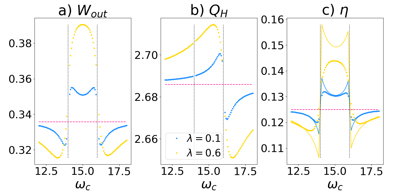
In Fig. 3 we show the behaviour of a) the total work output , b) the net heat input from the hot bath and c) the efficiency when varying (the position of the peak of the spectral densities of both the hot and the cold bath). The structure of the spectral density does not play a role in the Born-Markov approximation, therefore this parameter will only affect the exact dynamics. The pink dashed lines show the Born-Markov case for comparison, and we see that they remain constant for all . The dots show the results from the exact dynamics for different values of , for the weak coupling case (blue) and the strong coupling case (yellow). As expected, we observe that in the weak coupling regime the results are generally closer to the Born-Markov approximation than in the strong coupling regime.
We also look at the behaviour of work output, heat input and efficiency with varying for different values of the spectral width in Fig. 4. As can be seen from the second-order Born approximation in Equation (56), the value of also affects the coupling strength. This fact is reflected in the graph: For a narrow spectral density (blue lines) the results come closer to those from the Born-Markov approximation than for a wider one (yellow lines).
We note that in both cases shown in Figs. 3 and 4 when changing the work output deviates more strongly from the Born-Markov approximation than the heat input. In our numerical simulations we find this to be a general behaviour when varying parameters of the spectral density. Therefore, the behaviour of work with changing characteristics of the spectral density has a greater influence on the behaviour of the efficiency than that of heat.

Figures 3 and 4 clearly show a characteristic behaviour: Work output and efficiency are greater than in the Born-Markov case in the region , and smaller outside this region. The first intuition for this fact comes from Fig. 5, where we represent, for different values of , the Otto cycle in the -plane, where is the frequency of the oscillator and the mean occupation number. The colored solid curves represent the exact cycle, while the dashed black lines show the standard Born-Markov approximation. The area enclosed by the curves corresponds to the total work output. We can already see in this picture that the work output is higher for the case than in the Born-Markov approximation (Fig. 5b). This case corresponds to and and, consequently, to and , which results in the cycle taking place within a larger range of frequencies. For the cases (a) and (c) we see that the work output is smaller than in the standard approach, and that here the frequency renormalization reduces the work output, instead of enhancing it.
This behaviour of the work output translates into efficiency, which is also larger than the Born-Markov efficiency within the region . A simple approximation can be derived if we assume that within second order relaxes much more rapidly than . We see from (56) that relaxes on the time scale , while relaxes on the time scale , where is the Markovian relaxation rate given by Eq. (29), which yields in the present case . Thus, the assumption leads to the condition
| (57) |
Under this condition we can use (46) and (48) to get the approximate expressions
| (58) |
such that the efficiency of the cycle may be approximated by the renormalized effciency :
| (59) |
Note that is obtained from the Markovian efficiency (41) by replacing the bare frequencies with the renormalized frequencies. The renormalized efficiency (59) is represented by the solid lines in Figs. 3c and 4c. For the blue curves condition (57) is satisfied outside the resonances at , and we see that (59) indeed provides a good approximation for the cycle efficiency. Note that in the vicinity of the resonances () condition (57) is violated which explains why the approximation (59) is less accurate close to resonance.

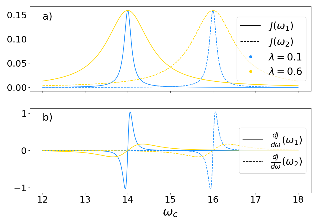
To further understand the curves shown in Figs. 3 and 4 we give an interpretation based on the height and the slope of the spectral density at the initial frequencies of the harmonic oscillator when coupled to each bath. In Figs. 6 and 7 we represented the height (top) and the slope (bottom) of the spectral density at (solid lines) and (dashed lines), i.e., and , with varying on the horizontal axis.
First, we will analyze the different behaviour of work output, heat input and efficiency for different values of the coupling strength . In Fig. 6 the lines show (blue) and (yellow), and all other parameters are the same as in Fig. 3. When we look at the curves in Fig. 3, we find, first of all, that the closer to resonance with the corresponding baths (), the more the results deviate from the standard Born-Markov approximation (except at exact resonance, see below), while far away from resonance the approximation predicts the results accurately. We can relate this to the fact that the height and the slope of the spectral density at close to resonance take significant values, while far away from resonance they have decayed to negligible quantities, and the bath looks flat in the vicinity of the initial frequency of the central harmonic oscillator. Additionally, we see that, for weak coupling (blue lines), presents a dip in the region , while for strong coupling (yellow lines) work output and efficiency have no inflection point in this region. If we look at the spectral densities for these two values of , we see that in the weak coupling regime the spectral densities and their slopes have decayed to negligible values for centrally located between and , while for strong coupling the spectral densities still take high values in this region, with significant slopes, and therefore strong effects in both the heating and the cooling phases combine. This is the reason why work output (and consequently efficiency) is maximally enhanced in this region for strong coupling. We also see that at resonance with either of the baths, the quantities seem to come close again to the Born-Markov approximation. If we look at the slope of the spectral densities in Fig. 6, we see that it vanishes as it approaches resonance (), resembling a flat bath.
In Fig. 7 the height (a) and slopes (b) of the spectral density at can be found for different values of , corresponding to the results shown in Fig. 4. The faster decay of the spectral density and its slope for small (blue) can account for the higher resemblance of the results to those in the Born-Markov approximation far from resonance. On the contrary, for large (yellow) the cycle is most altered for intermediate between and , when the height and slope of both and are still significant, meaning that both the heating and the cooling phases feel the effects of a strongly coupled, structured bath.

We now turn to look at the different modes of operation of the cycle in different parameter ranges. In the standard Born-Markov approximation this distinction is clear: The cycle operates as a heat engine ( and ) for the configurations of frequencies and temperatures that satisfy (42), and as a refrigerator ( and ) otherwise (due to the fact that work output and heat input change sign at the same points). In the exact approach we can only determine the behaviour of the cycle numerically, and it will additionally depend on the specific parameters of the spectral density. We find that the exact approach can give rise to three different types of behaviour: As a heat engine or refrigerator as before, but also as a heater ( and ), where the cycle just uses work to amplify the flow of heat from the hot to the cold reservoir.
In Fig. 8 we depict the regions in which the cycle operates as a heat engine (green), as a refrigerator (blue) or as a heater (red). The dashed black lines represent the limit between the heat engine and the refrigerator regions in the standard Born-Markov approximation. On the horizontal axis we change , where we have chosen a reference temperature and vary the temperatures of the cold and the hot bath symmetrically such that . On the vertical axis we change , where we have chosen a as the reference frequency and vary . It can be observed that in the exact approach the region in which the cycle operates as a heat engine is limited compared to the Born-Markov case, with work output being positive for a smaller range of frequencies and temperatures. For small and this difference is almost negligible, but it increases as we increase and . Additionally, a new type of behaviour appears and expands as and increase: The cycle operates as a heater, where a work input is used to dissipate heat from the hot reservoir into the cold reservoir. In spite of this, for large values of and (Fig. 8d) the refrigerator region broadens.

Finally, we analyze the values of and for which we can obtain the highest efficiencies. From Figs. 3 and 4 it may seem that, for a spectral density satisfying , the higher the parameters or are, the higher is the efficiency. However, in Fig. 9 we show the efficiency as a function of both and for a spectral density centered between and , and we see that the behaviour of is not monotonic with increasing or . We observe that, fixing one parameter, there exists an optimal value of the other parameter such that the efficiency is maximal. We show the results for two different temperatures of the hot bath , and it can be seen that the values of and for which the efficiency is maximal change with temperature. Therefore, stronger coupling can enhance the efficiency of the cycle, but only up to a limit, at which point it starts being a hindrance. Larger spectral width can also start improving the efficiency, as the spectral density gets wider and starts having relevant effects on both the heating and cooling phases. However, if becomes too large, the slope of the spectral density decreases, resembling a flat, Markovian bath and resulting in a lower efficiency for the cycle.
IV Conclusions
We have investigated the thermodynamics of the quantum Otto cycle in the presence of non-Markovian effects and strong system-bath coupling. Our analysis was based on a novel approach to quantum thermodynamics, which allowed us to exactly resolve the consequences of coupling a system to an arbitrary reservoir with memory effects. By comparing the standard Markovian Otto cycle with the exact non-Markovian treatment, we have identified feasible conditions under which the cycle exhibits enhanced work output and efficiency. These enhancements occur when the spectral density of the bath peaks at a frequency which is located within the driving range of the system, leading to an effective broadening of the range of frequencies in which the cycle operates. Conversely, outside these regions, the cycle performance either is lower or remains close to the standard Born-Markov approximation. When taking baths with a spectral density that enhances the efficiency, we encounter a small trade-off in the parameter region of frequencies and temperatures for which the cycle is producing work output, but this effect becomes noticeable only at very large coupling parameters. We have also shown that the behaviour of work output and efficiency strongly depends on the strength of the system-bath coupling and the width of the spectral density, showcasing how much the nuances of the bath spectral density can influence the performance of the cycle.
It is important to acknowledge that our analysis focused solely on the quantum Otto cycle. Further research is required to investigate the implications of memory effects in other quantum thermal machine models and explore their influence on diverse thermodynamic processes. Still, the present study highlights the role of memory effects and structured environments as a promising avenue for the enhancement of current quantum thermal machines – one notable implication of our findings being the potential for exploiting strong system-bath coupling to achieve more efficient quantum heat engines.
While in this work we have not concerned ourselves with the duration of the cycle – allowing fully adiabatic driving and infinitely long thermalization times – this could in principle represent another positive aspect of considering reservoirs outside of the weak-coupling regimes. A promising path would be to investigate how the coupling strength can influence thermalization rates, possibly leading to shorter relaxation times and, in turn, higher efficiencies at maximum power. Moreover, while we have demonstrated enhancements in performance for specific scenarios, it still warrants exploration whether surpassing the Carnot efficiency is feasible with non-Markovian baths.
Acknowledgements.
This project has received funding from the European Union’s Framework Programme for Research and Innovation Horizon 2020 (2014-2020) under the Marie Skłodowska-Curie Grant Agreement No. 847471. The work has also been supported by the German Research Foundation (DFG) through FOR 5099.Appendix A Derivation of the exact master equation
We present some details on to derivation of the time-convolutionless exact master equation of the form (2) with effective Hamiltonian (24) and dissipator (25) for the microscopic model discussed in Sec. II.2. This master equation has been obtained in Tu and Zhang 2008; Jin et al. 2010; Lei and Zhang 2012 using path integral techniques. Here, we show how to derive it directly from the exact expressions (20)-(22) for the first and second moments. To this end, we first take the time derivatives to find the following exact equations of motion for these moments:
| (60) | |||||
| (61) | |||||
| (62) | |||||
Since the microscopic Hamiltonian is quadratic we know that the dynamics preserves the Gaussianity of states and, hence, that the master equation must be quadratic in the creation and annihilation operators , of the central oscillator. The strategy is thus to write a suitable quadratic ansatz for the generator of the master equation and to chose the coefficients in such a way that the moment equations obtained from the master equation coincide with Eqs. (60)-(62). If we have found such an ansatz, we can conclude that it yields the correct exact generator of the master equation.
Our ansatz for the master equation takes the form
| (63) |
where (compare to Eqs. (24) and (25))
| (64) |
and
| (65) | |||||
with five time dependent coefficients , , , and . The coefficients , and must be real because the master equation must preserve the Hermiticity of the density matrix. This ansatz yields the following equation for the first moment,
| (66) |
and the comparison with (60) leads to
| (67) | |||||
| (68) | |||||
| (69) |
where we have used the definitions (26) and (27). From the master equation (63) we also obtain:
| (70) |
The comparison with (62) leads to the additional condition
| (71) |
where we have used definition (28). This equation also yields
| (72) |
Finally, we find from the master equation (63):
| (73) |
which in view of (61) gives
| (74) |
With Eqs. (67), (69), (71), (72) and (74) we have determined all five coefficients of the master equation (63), and the latter is easily seen to coincide with the master equation (2).
Appendix B Spectral density
The spectral density must decrease to zero sufficiently rapidly for in order for the noise integral to be finite. This can be seen by rewriting , which is defined in Eq. (23), as follows
| (75) |
where is the initial Planck distribution of the environmental modes, resulting from the assumption that the bath is initially in a thermal equilibrium state (see Eq. (17)), which behaves as for small frequencies. To guarantee that the frequency integral converges for , we replace the Lorentzian spectral density in (75) by the spectral density which shows a linear behavior for low frequencies below a certain threshold :
| (76) |
We find that this procedure is consistent as long as the condition
| (77) |
holds. This condition can be obtained by expressing the Laplace transform of in terms of the spectral density and by requiring that the replacement has only negligible impact on (75).
References
- Abah et al. (2012) O. Abah, J. Roßnagel, G. Jacob, S. Deffner, F. Schmidt-Kaler, K. Singer, and E. Lutz, Phys. Rev. Lett. 109, 203006 (2012).
- Roßnagel et al. (2016) J. Roßnagel, S. T. Dawkins, K. N. Tolazzi, O. Abah, E. Lutz, F. Schmidt-Kaler, and K. Singer, Science 352, 325 (2016).
- de Assis et al. (2019) R. J. de Assis, T. M. de Mendonça, C. J. Villas-Boas, A. M. de Souza, R. S. Sarthour, I. S. Oliveira, and N. G. de Almeida, Phys. Rev. Lett. 122, 240602 (2019).
- von Lindenfels et al. (2019) D. von Lindenfels, O. Gräb, C. T. Schmiegelow, V. Kaushal, J. Schulz, M. T. Mitchison, J. Goold, F. Schmidt-Kaler, and U. G. Poschinger, Phys. Rev. Lett. 123, 080602 (2019).
- Peterson et al. (2019) J. P. S. Peterson, T. B. Batalhão, M. Herrera, A. M. Souza, R. S. Sarthour, I. S. Oliveira, and R. M. Serra, Phys. Rev. Lett. 123, 240601 (2019).
- Myers et al. (2022) N. M. Myers, O. Abah, and S. Deffner, AVS Quantum Science 4, 027101 (2022).
- Breuer et al. (2016) H.-P. Breuer, E.-M. Laine, J. Piilo, and B. Vacchini, Rev. Mod. Phys. 88, 021002 (2016).
- Weimer et al. (2008) H. Weimer, M. J. Henrich, F. Rempp, H. Schröder, and G. Mahler, EPL (Europhysics Letters) 83, 30008 (2008).
- Esposito et al. (2010) M. Esposito, K. Lindenberg, and C. V. den Broeck, New Journal of Physics 12, 013013 (2010).
- Teifel and Mahler (2011) J. Teifel and G. Mahler, Phys. Rev. E 83, 041131 (2011).
- Alipour et al. (2016) S. Alipour, F. Benatti, F. Bakhshinezhad, M. Afsary, S. Marcantoni, and A. T. Rezakhani, Sci. Rep. 6, 35568 (2016).
- Seifert (2016) U. Seifert, Phys. Rev. Lett. 116, 020601 (2016).
- Strasberg et al. (2017) P. Strasberg, G. Schaller, T. Brandes, and M. Esposito, Phys. Rev. X 7, 021003 (2017).
- Rivas (2020) A. Rivas, Phys. Rev. Lett. 124, 160601 (2020).
- Alipour et al. (2022) S. Alipour, A. T. Rezakhani, A. Chenu, A. del Campo, and T. Ala-Nissila, Phys. Rev. A 105, L040201 (2022).
- Landi and Paternostro (2021) G. T. Landi and M. Paternostro, Rev. Mod. Phys. 93, 035008 (2021).
- Strasberg and Esposito (2019) P. Strasberg and M. Esposito, Phys. Rev. E 99, 012120 (2019).
- Colla and Breuer (2021) A. Colla and H.-P. Breuer, Phys. Rev. A 104, 052408 (2021).
- Zhang et al. (2014) X. Y. Zhang, X. L. Huang, and X. X. Yi, Journal of Physics A: Mathematical and Theoretical 47, 455002 (2014).
- Pozas-Kerstjens et al. (2018) A. Pozas-Kerstjens, E. G. Brown, and K. V. Hovhannisyan, New Journal of Physics 20, 043034 (2018).
- Thomas et al. (2018) G. Thomas, N. Siddharth, S. Banerjee, and S. Ghosh, Phys. Rev. E 97, 062108 (2018).
- Pezzutto et al. (2019) M. Pezzutto, M. Paternostro, and Y. Omar, Quantum Science and Technology 4, 025002 (2019).
- Mukherjee et al. (2020) V. Mukherjee, A. G. Kofman, and G. Kurizki, Communications Physics 3, 8 (2020).
- Wiedmann et al. (2020) M. Wiedmann, J. T. Stockburger, and J. Ankerhold, New Journal of Physics 22, 033007 (2020).
- Wiedmann et al. (2021) M. Wiedmann, J. T. Stockburger, and J. Ankerhold, The European Physical Journal Special Topics 230, 851 (2021).
- Chakraborty et al. (2022) S. Chakraborty, A. Das, and D. Chruściński, Phys. Rev. E 106, 064133 (2022).
- Kaneyasu and Hasegawa (2023) M. Kaneyasu and Y. Hasegawa, Phys. Rev. E 107, 044127 (2023).
- Ishizaki et al. (2023) M. Ishizaki, N. Hatano, and H. Tajima, Phys. Rev. Res. 5, 023066 (2023).
- Liu et al. (2021) J. Liu, K. A. Jung, and D. Segal, Phys. Rev. Lett. 127, 200602 (2021).
- Colla and Breuer (2022) A. Colla and H.-P. Breuer, Phys. Rev. A 105, 052216 (2022).
- Kosloff and Rezek (2017) R. Kosloff and Y. Rezek, Entropy 19 (2017), 10.3390/e19040136.
- Fano (1961) U. Fano, Phys. Rev. 124, 1866 (1961).
- Anderson (1961) P. W. Anderson, Phys. Rev. 124, 41 (1961).
- Mahan (2000) G. D. Mahan, Many-Particle Physics (Kluwer Academic/Plenum Publishers, New York, 2000).
- Huang and Zhang (2022a) W.-M. Huang and W.-M. Zhang, Phys. Rev. Res. 4, 023141 (2022a).
- Huang and Zhang (2022b) W.-M. Huang and W.-M. Zhang, Phys. Rev. A 106, 032607 (2022b).
- Shibata et al. (1977) F. Shibata, Y. Takahashi, and N. Hashitsume, J. Stat. Phys. 17, 171 (1977).
- Chaturvedi and Shibata (1979) S. Chaturvedi and F. Shibata, Z. Phys. B 35, 297 (1979).
- Hall et al. (2014) M. J. W. Hall, J. D. Cresser, L. Li, and E. Andersson, Phys. Rev. A 89, 042120 (2014).
- Breuer (2012) H.-P. Breuer, J. Phys. B 45, 154001 (2012).
- Breuer and Petruccione (2002) H.-P. Breuer and F. Petruccione, The Theory of Open Quantum Systems (Oxford University Press, Oxford, 2002).
- van Kampen (1974a) N. G. van Kampen, Physica 74, 215 (1974a).
- van Kampen (1974b) N. G. van Kampen, Physica 74, 239 (1974b).
- Tu and Zhang (2008) M. W. Y. Tu and W.-M. Zhang, Phys. Rev. B 78, 235311 (2008).
- Jin et al. (2010) J. Jin, M. W.-Y. Tu, W.-M. Zhang, and Y. Yan, New Journal of Physics 12, 083013 (2010).
- Lei and Zhang (2012) C. U. Lei and W.-M. Zhang, Annals of Physics 327, 1408 (2012).
- Zhang et al. (2012) W.-M. Zhang, P.-Y. Lo, H.-N. Xiong, M. W.-Y. Tu, and F. Nori, Phys. Rev. Lett. 109, 170402 (2012).
- Sorce and Hayden (2022) J. Sorce and P. M. Hayden, J. Phys. A: Math. Theor. (2022), 10.1088/1751-8121/ac65c2.
- (49) We remark that an extension of our approach to correlated initial states seems possible by means of the formalism developed in Colla et al. 2022.
- Deffner and Lutz (2008) S. Deffner and E. Lutz, Phys. Rev. E 77, 021128 (2008).
- Husimi (1953) K. Husimi, Prog. Theor. Phys. 9, 381 (1953).
- Shirai et al. (2021) Y. Shirai, K. Hashimoto, R. Tezuka, C. Uchiyama, and N. Hatano, Phys. Rev. Res. 3, 023078 (2021).
- Latune et al. (2023) C. L. Latune, G. Pleasance, and F. Petruccione, “Cyclic quantum engines enhanced by strong bath coupling,” (2023), arXiv:2304.03267 [quant-ph] .
- Colla et al. (2022) A. Colla, N. Neubrand, and H.-P. Breuer, New Journal of Physics 24, 123005 (2022).