跳到论文正文
W Papers独立论文阅读器 arXiv:2308.09006 论文正文 计算阅读时间 · 0%
引用这篇论文根据当前论文元数据生成,正式投稿前建议核对。


License: arXiv.org perpetual non-exclusive license
arXiv:2308.09006v2 [hep-th] 30 Nov 2023

YITP-23-104

Unitarity Violation in Field Theories of

Lee-Wick’s Complex Ghost

Jisuke Kubo,1,2,** * e-mail address: kubo@mpi-hd.mpg.de and Taichiro Kugo,3,†† † e-mail address: kugo@yukawa.kyoto-u.ac.jp

1 Max-Planck-Institut für Kernphysik(MPIK), Saupfercheckweg 1, 69117 Heidelberg, Germany

2 Department of Physics, University of Toyama, 3190 Gofuku, Toyama 930-8555, Japan

3 Center for Gravitational Physics and Quantum Information,
Yukawa Institute for Theoretical Physics, Kyoto University, Kyoto 606-8502, Japan

Abstract

Theories with fourth-order derivatives, including the Lee-Wick finite QED model and Quadratic Gravity, have a better UV behaviour, but the presence of negative metric ghost modes endanger unitarity. Noticing that the ghost acquires a complex mass by radiative corrections, Lee and Wick, in particular, claimed that such complex ghosts would never be created by collisions of physical particles because of energy conservation, so that the physical S-matrix unitarity must hold.

We investigate the unitarity problem faithfully working in the operator formalism of quantum field theory. When complex ghosts participate, a complex delta function (generalization of Dirac delta function) appears at each interaction vertex, which enforces a specific conservation law of complex energy. Its particular property implies that the naive Feynman rule is wrong if the four-momenta are assigned to the internal lines after taking account of the conservation law in advance. We show that the complex ghosts are actually created and unitarity is violated in such fourth-order derivative theories. We also find a definite energy threshold below which the ghosts cannot be created: The theories are unitary and renormalizable below the threshold.

I Introduction

It has long been a challenge to construct a consistent quantum filed theory (QFT) of gravity, though a well-known candidate is Quadratic Gravity (QG) whose renormalizability was proven by Stelle Stelle:1976gc long ago. The action of QG contains in addition to the Einstein-Hilbert term RR, the Weyl tensor squared Cμ​ν​ρ​σ2C_{\mu\nu\rho\sigma}^{2} as well as R2R^{2} (see e.g. Mannheim:2011ds; Salvio:2018crh for a review). The canonical dimension of these two terms is four, which means that any renormalizable QFT of gravity will contain them tHooft:2011aa. The main reason that QG is renormalizable is that it has a built-in ultraviolet (UV) regulator, the spin-two ghost field Stelle:1976gc, which however endangers the unitarity of the theory. The origin of the good side and the bad side is the same; fourth-order derivatives in the equations of motion. The propagator of a fourth-order theory can be written as a sum of two propagators of a second-order theory, where one of them must come with an opposite sign, where the wrong-sign propagator originates from the wrong sign of the kinetic term. This implies that there exists a negative-metric ghost. 11 1 That is, we have to deal with an indefinite metric space when the theory is quantized Boulware:1983td, instead of the classical Ostrogradsky instability problem Ostrogradsky:1850fid; Woodard:2015zca. Our interest in this paper is focused on this troublesome feature, and we shall investigate the unitarity problem in great detail.

Long before Stelle’s proof for renormalizability of QG, Lee and Wick Lee:1969fy; Lee:1969zze; Lee:1970iw used the aforementioned built-in mechanism to soften the UV behavior of QFT. They considered a QED-like theory Lee:1970iw with a spin-one massive ghost field and made a very remarkable observation: The radiative corrections to the ghost propagator due to light fermion (e.g., lepton pair) loops makes the single pole split into two complex conjugate poles. That is, the mass and energy of the ghost become complex. This fact became an essential part of their proof of the unitarity: Ghosts cannot be produced in a scattering process of physical particles possessing real energies because of the conservation of energy (in particular, because of the conservation of the imaginary part of the energy). 22 2 This reasoning has been tacitly approved also by, e.g., Coleman Coleman:1969xz and Nakanishi Nakanishi:1971jj; Gleeson:1971cvx, despite the fact that Coleman pointed out a possible violation of causality in the presence of indefinite-metric ghosts, and that Nakanishi showed violation of Lorentz invariance in the Lee-Wick prescription of how to integrate the internal momenta. If the ghosts are not produced from any physical initial states, the unitarity of the S-matrix restricted to the physical particles alone, i.e., the physical unitarity, holds. Although this physical intuition sounds correct, it seems that Feynman diagrams do not share this intuition since one has to give a precise prescription how to integrate internal momenta Lee:1969fy; Lee:1969zze; Lee:1970iw; Cutkosky:1969fq. In fact, how to choose an appropriate integration contour in the complex energy plane has been the target of theoretical physicists since then and even recently Anselmi:2017ygm; Anselmi:2018kgz; Donoghue:2019fcb; Donoghue:2021eto. 33 3 There are a number of other interesting attempts to show the unitarity, see for instance Bender:2007wu; Bender:2007nj; Grinstein:2008bg; Mannheim:2018ljq; Salvio:2019wcp; Platania:2020knd; Platania:2022gtt. However, to our knowledge, none of them are solely based on QFT because certain assumptions have to be made and it is not clear that they are consistent in QFT, especially in the presence of interactions such as gravity. The approach described above is based on the standpoint that a theory is defined by its Feynman expansion Coleman:1969xz.

Our interest in this paper is to investigate the aforementioned unitarity problem solely based on QFT. We will use the tools of QFT, no more, no less. How to integrate the loop momenta in a Feynman diagram, apart from its regularization, is dictated by QFT with no room left for speculation. If energy is complex, we encounter a mathematical expression, a complex distribution, which to our knowledge has not been sufficiently explored so far aside from a brief discussion in Nakanishi’s work Nakanishi:1958; Nakanishi:1958-2; Nakanishi:1972wx. It is just the integral

limT→∞12​π​∫−TTd​t​e−i​E​t=:δc​(E),\lim_{T\to\infty}\,\frac{1}{2\pi}\int_{-T}^{T}dt\,e^{-iEt}=:\delta_{\rm c}(E)\,, (1)

which appears at each vertex, where EE is the sum ∑iEi\sum_{i}E_{i} of the energies of particles ii entering the vertex. If the energy EE is real, the limit T→∞T\to\infty is the Dirac delta function, as we all know. But what is the limit if EE is complex? Nakanishi Nakanishi:1958; Nakanishi:1958-2; Nakanishi:1972wx called it a complex delta function and derived some of its mathematical properties, but he did not recognize that the complex distribution plays an essential role in investigating unitarity. The integral (1) with a complex EE appears at each vertex of the Dyson expansion in perturbation theory if ghost lines are attached. Usually, we do not care about this integral because it just gives a delta function which expresses the energy conservation at each vertex. Thus, the mathematical property of the integral (1) is intimately related to the energy conservation, especially in the case that the energy is complex. Or, speaking more strongly, the property of the complex delta function (or distribution) defined by the integral (1) is all of the content of the “energy conservation law” in the case where complex ghosts participate.

We will see that δc​(E)\delta_{\rm c}(E) is non-vanishing even when Im​E≠0{\rm Im}\,E\not=0, thus implying that ghosts can be produced with finite (i.e., non-zero) probability through a collision of physical particles. This leads us to the conclusion that the physical unitarity of the S-matrix in fourth-order derivative theories such as the Lee-Wick finite QED and QG is violated in QFT. 44 4 By the physical unitarity we mean that the probability interpretation of quantum theory is possible. The physical unitarity of the S-matrix should be distinguished from the total S-matrix unitarity (S†​S=S​S†=1CLOSE(S^{\dagger}S=SS^{\dagger}=1) which is satisfied if the Hamiltonian is hermitian. In the following discussions we sometimes suppress “physical” if it does not lead to a confusion. A positive message, however, is that these theories are good effective theories in the sense that the physical unitarity of the S-matrix is satisfied below a definite threshold energy for the ghost production, where internal ghost propagators in a Feynman diagram may still be present. 55 5 Because of the imaginary part of the complex mass, the meaning of the threshold should be slightly modified.

In connection with the property of the complex delta function, we should mention a very important point which invalidates the usual Feynman rule with energy-momentum conservation used at each vertex in advance. For instance, consider a self-energy type one-loop diagram consisting of a physical particle ψ\psi with real mass squared μ2\mu^{2} and a ghost φ\varphi with complex mass squared M2M^{2}. Many would naively write down the expression

Σ⁡(p)∝∫d4​q​Dφ​(q)​Dψ​(p−q)=∫d4​q​1q2+M2​1(p−q)2+μ2,\Sigma(p)\propto\int d^{4}qD_{\varphi}(q)\,D_{\psi}(p-q)\,=\int d^{4}q\,\frac{1}{q^{2}+M^{2}}\,\frac{1}{(p-q)^{2}+\mu^{2}}\,, (2)

but this is wrong! T. D. Lee also started with this expression and correctly calculated this integral, even taking the deformed q0q^{0}-integration contour into account properly, and reached the conclusion that the amplitude has no imaginary part so that the production of a ghost φ\varphi and a physical particle ψ\psi would not occur. This is an incorrect conclusion obtained from a correct calculation but from the wrong starting expression. The correct expression is not Eq. (2), but

Σ⁡(p)∝∫d4​k​d4​q​Dφ​(q)​Dψ​(k)​δc​(k0+q0−p0)​δ3​(𝒌+𝒒−𝒑).\Sigma(p)\propto\int d^{4}k\,d^{4}q\,D_{\varphi}(q)\,D_{\psi}(k)\,\delta_{\rm c}(k^{0}+q^{0}-p^{0})\delta^{3}({\bm{k}}+{\bm{q}}-{\bm{p}})\,. (3)

The k0k^{0}-integration of the complex delta function δc​(k0+q0−p0)\delta_{\rm c}(k^{0}+q^{0}-p^{0}) does not give the substitution rule k0→p0−q0k^{0}\rightarrow p^{0}-q^{0} alone when the multiplied function is not analytic in k0k^{0}. In the usual Feynman graph case, the multiplied function is the propagator, here Dψ​(k)D_{\psi}(k), which is not analytic but meromorphic in k0k^{0}. The pole singularities also give additional contributions.

This problem is serious since the Feynman rules with energy-momentum conservation like in Eq. (2) are already assumed in all the approaches discussing the integration contours in the complex energy plane. This implies that those approaches have no ground in QFT.

We organize the paper as follows. In order to discuss the complex ghost problem properly in QFT, we adopt in this paper Lee’s purely scalar field theory model Lee:1969zze, which Lee devised to mimic the essential features of the fourth-order derivative system like finite QED or QG. We will present the Lee model in Section II and its quantization as an indefinite metric QFT in the manner given by Nakanishi Nakanishi:1972wx. In particular, we will explain the unfamiliar metric structure of the complex ghost field φ\varphi and derive two expressions for the ghost propagator; the 3​d3d and 4​d4d momentum expressions. In the latter, as we shall see, the integration contour of the zeroth component k0k^{0} must take a detour around the complex poles that is much deviated from the real axis. This causes a considerable complication in the Feynman diagram computations despite the apparently covariant compact 4​d4d-momentum expressions.

Our main concern is whether the ghost and anti-ghost are really created in the scattering processes of physical particles. In Section III, we examine the simplest process of single ghost/anti-ghost production by the scattering of two physical particles, ψ+ψ→φ/φ†\psi+\psi\rightarrow\varphi/\varphi^{\dagger}. We calculate this production probability to the lowest order in three ways. First is the direct calculation of the production amplitude, given in subsection III.1, which is almost trivial and simply given by the complex delta function δc\delta_{\rm c}, so we give its precise definition and derive some basic properties in subsection III.2. We then explicitly show that the ghost is actually produced with non-vanishing probability by the two physical particle scattering if the incident energy EE is above Re​M2−Im​M2{\rm Re}\,\sqrt{M^{2}}-{\rm Im}\,\sqrt{M^{2}} (lower threshold) and below Re​M2+Im​M2{\rm Re}\,\sqrt{M^{2}}+{\rm Im}\,\sqrt{M^{2}} (upper threshold) with M2M^{2} being the complex mass squared of the ghost.

Although this is enough for a proof of ghost appearance, we also calculate this production probability in subsection III.3 by computing the imaginary part of the forward scattering amplitude of ψ+ψ→ψ+ψ\psi+\psi\rightarrow\psi+\psi with the ghost/anti-ghost intermediate line (propagator) in the ss-channel. We present two methods of computation for this by using 3​d3d- and 4​d4d-momentum expressions for the ghost propagator in subsubsections III.3.1 and III.3.2. These calculations give the same result as the direct calculation in subsection III.1, as a result of the optical theorem. These calculations are presented not only for checking the mutual consistency between various ways of calculation, but also for showing how the calculations of Feynman graphs should be performed in the presence of complex ghost fields and complex delta functions.

We consider a two ghost production process from a two physical particle scattering in Section IV. The direct calculation of the production probability is the simplest, but it is deferred to subsection IV.2. In the first subsection IV.1, we present the calculation of the forward scattering amplitude ψ+ψ→ψ+ψ\psi+\psi\rightarrow\psi+\psi at one-loop in which a pair of ghosts/anti-ghosts circulates. We present this to demonstrate how the proper calculation goes since this type of loop diagram has been discussed by many others, whose calculations often have the problem mentioned above in Eq. (2) already at the starting expression. The calculation using 3​d3d-momentum expression for the ghost propagator is presented in subsubsection IV.1.1, which is simpler compared with the one using 4​d4d-momentum expression presented in IV.1.2. The latter calculation is actually rather tough and lengthy and its main body has been moved to the Appendix. Instead, we add there a concise explanation for the reason why the naive Feynman rule (2) is wrong and how it should be modified, since such explanations given for many examples are buried in the lengthy calculations moved to the Appendix.

Those three ways of computation give the same result as given in subsection IV.2 for the production probability of a ghost pair. This result contains the complex delta function which is integrated with respect to the 3-momentum 𝒒{\bm{q}} of ghosts. Since the complex delta function indirectly depends on 𝒒{\bm{q}} through the ghost energy ω𝒒=𝒒2+M2\omega_{\bm{q}}=\sqrt{{\bm{q}}^{2}+M^{2}} as δc​(E−ω𝒒)\delta_{\rm c}(E-\omega_{\bm{q}}), the qq-integration reveals a new interesting aspect of the complex delta function δc\delta_{\rm c}. So, in subsection IV.3, we discuss how to evaluate the qq-integral and obtain the clear result that the production probability vanishes for the incident energy below the lower threshold and becomes a well-defined finite value for energy above the upper threshold. For energy EE between the upper and lower thresholds, the result is divergent though the smearing of the incident energy with any finite width gives a well-defined production probability, as is usual for the distribution.

Section V is devoted to the conclusion.

II Lee’s Model

In order to examine the properties of complex ghost fields in as simple a manner as possible, Lee devised in Ref.  Lee:1969zze a purely scalar field model which mimics the essential features of the Lee-Wick’s finite QED theory in this respect. We call it Lee’s model here and explain this model in a clear manner as Nakanishi presented in Ref.  Nakanishi:1972wx.

The system consists of three real scalar fields A,BA,B and CC in the ‘photon’ sector and a normal scalar field ψ\psi in the matter sector, whose free Lagrangian is given by

ℒfree\displaystyle{\cal L}_{\rm free} =ℒABC+ℒmatter,\displaystyle={\cal L}_{\rm ABC}+{\cal L}_{\rm matter}\,, (4)
ℒABC\displaystyle{\cal L}_{\rm ABC} =−12​[(∂μA)2+δ2​A2]+12​[(∂μB)2+m2​B2]−12​[(∂μC)2+m2​C2]−γ2​B​C,\displaystyle=-\frac{1}{2}\left[(\partial_{\mu}A)^{2}+\delta^{2}A^{2}\right]+\frac{1}{2}\left[(\partial_{\mu}B)^{2}+m^{2}B^{2}\right]-\frac{1}{2}\left[(\partial_{\mu}C)^{2}+m^{2}C^{2}\right]-\gamma^{2}BC\,,
ℒmatter\displaystyle{\cal L}_{\rm matter} =−12​(∂μψ)2−12​μ2​ψ2.\displaystyle=-\frac{1}{2}(\partial_{\mu}\psi)^{2}-\frac{1}{2}\mu^{2}\psi^{2}\,. (5)

Here, A⁡(x)A(x) is an analogue of the ‘photon’ AμA_{\mu} in QED that possesses a small mass δ\delta, and B⁡(x)B(x) is a negative metric regulator field with a large mass mm accompanying the ‘photon’ AA. The C⁡(x)C(x) (which mixes with BB and is absent in the original Lee-Wick QED) is introduced to simulate the continuum states like lepton pairs, e+​e−e^{+}e^{-} and μ+​μ−\mu^{+}\mu^{-}. The mixing is represented by the last term −γ2​B​C-\gamma^{2}BC. We are using the space-favored metric ημ​ν=diag⁡(−1,+1,+1,+1)\eta_{\mu\nu}={\rm diag}(-1,+1,+1,+1), so that the ‘photon’ AA and continuum CC fields, as well as the matter field ψ\psi, are of positive metric while the regulator BB is of negative metric. We also note that all the fields are real (i.e., hermitian)66 6 Our BB field here stands for ii times Lee’s BB field; Bhere=i​BLeeB_{\rm here}=iB_{\rm Lee}. We also avoid the use of the extraneous (and sometimes confusing) metric operator η\eta to treat negative metric field BB. Lee’s η−1​ϕ†​η\eta^{-1}\phi^{\dagger}\eta is simply our ϕ†\phi^{\dagger}., and that the Lagrangian (5) is hermitian if the mass parameters δ\delta, mm and the BB-CC mixing γ\gamma are real.

The B​CBC sector of the free field Lagrangian can also be diagonalized by introducing the following complex ghost field φ⁡(x)\varphi(x):77 7 This complex ghost field φ⁡(x)\varphi(x) multiplied by ii is Nakanishi’s field ϕ=(φ1+i​φ2)/2\phi=(\varphi_{1}+i\varphi_{2})/\sqrt{2} originally introduced in Ref.Nakanishi:1972wx. His φ1\varphi_{1} and φ2\varphi_{2} are Lee’s CC and BB, respectively.

φ=12​(B−i​C)or{B=(φ+φ†)/2C=i⁡(φ−φ†)/2.\displaystyle\varphi=\frac{1}{\sqrt{2}}(B-iC)\qquad\hbox{or}\qquad\begin{cases}B=(\varphi+\varphi^{\dagger})/\sqrt{2}&\\ C=i(\varphi-\varphi^{\dagger})/\sqrt{2}\end{cases}\ . (6)

Then, we have

ℒB​C\displaystyle{\cal L}_{BC} =\displaystyle= 12​[(∂μB)2−(∂μC)2+m2​(B2−C2)−2​γ2​B​C]\displaystyle\frac{1}{2}\left[(\partial_{\mu}B)^{2}-(\partial_{\mu}C)^{2}+m^{2}(B^{2}-C^{2})-2\gamma^{2}BC\right] (7)
=\displaystyle= 12​[∂μφ​∂μφ+M2​φ2+∂μφ†​∂μφ†+M∗2​φ†2],\displaystyle\frac{1}{2}\left[\partial_{\mu}\varphi\,\partial^{\mu}\varphi+M^{2}\varphi^{2}+\partial_{\mu}\varphi^{\dagger}\,\partial^{\mu}\varphi^{\dagger}+{M^{*}}^{2}{\varphi^{\dagger}}^{2}\right],

where the mass squared M2M^{2} for the φ\varphi field now takes a complex value:

M2=m2+i​γ2.M^{2}=m^{2}+i\gamma^{2}\,. (8)

As shown by Nakanishi Nakanishi:1972wx, the complex ghost field φ\varphi can be canonically quantized and is expanded as

φ⁡(x)=∫d3​𝒒(2​π)3​2​ω𝒒​(α⁡(𝒒)​ei​𝒒​𝒙−i​ω𝒒​x0+β†​(𝒒)​e−i​𝒒​𝒙+i​ω𝒒​x0),\varphi(x)=\int\frac{d^{3}{\bm{q}}}{\sqrt{(2\pi)^{3}2\omega_{{\bm{q}}}}}\left(\alpha({\bm{q}})e^{i{\bm{q}}{\bm{x}}-i\omega_{{\bm{q}}}x^{0}}+\beta^{\dagger}({\bm{q}})e^{-i{\bm{q}}{\bm{x}}+i\omega_{{\bm{q}}}x^{0}}\right)\,, (9)

where ω𝒒\omega_{{\bm{q}}} is the complex energy

ω𝒒=𝒒2+M2=𝒒2+m2+i​γ2,\omega_{{\bm{q}}}=\sqrt{{\bm{q}}^{2}+M^{2}}=\sqrt{{\bm{q}}^{2}+m^{2}+i\gamma^{2}}\,, (10)

and the creation and annihilation operators satisfy the off-diagonal commutation relations:88 8 Since i​φhere​(x)=ϕNakanishi​(x)i\varphi_{\rm here}(x)=\phi_{\rm Nakanishi}(x), our creation and annihilation operators differ from Nakanishi’s by a factor of ii as αhere​(𝒒)=−i​αNakanishi​(𝒒)\alpha_{\rm here}({\bm{q}})=-i\alpha_{\rm Nakanishi}({\bm{q}}) and βhere​(𝒒)=i​βNakanishi​(𝒒)\beta_{\rm here}({\bm{q}})=i\beta_{\rm Nakanishi}({\bm{q}}).

[α⁡(𝒑),β†​(𝒒)]=[β⁡(𝒑),α†​(𝒒)]=−δ3​(𝒑−𝒒),\displaystyle[\alpha({\bm{p}}),\beta^{\dagger}({\bm{q}})]=[\beta({\bm{p}}),\alpha^{\dagger}({\bm{q}})]=-\delta^{3}({\bm{p}}-{\bm{q}})\,,
[α⁡(𝒑),α†​(𝒒)]=[β⁡(𝒑),β†​(𝒒)]=0.\displaystyle[\alpha({\bm{p}}),\alpha^{\dagger}({\bm{q}})]=[\beta({\bm{p}}),\beta^{\dagger}({\bm{q}})]=0\,. (11)

The Hamiltonian in the BC sector is constructed as usual from the Lagrangian (7) and is given by

HBC\displaystyle H_{\rm BC} =\displaystyle= ∫d3𝒙(−12)[πφ2+∇φ⋅∇φ+h.c.]\displaystyle\int d^{3}{\bm{x}}\Big(-\frac{1}{2}\Big)\left[\pi^{2}_{\varphi}+\nabla\varphi\cdot\nabla\varphi+{\rm h.c.}\right] (12)
=\displaystyle= ∫d3​𝒑​[−ω𝒑​β†​(𝒑)​α​(𝒑)−ω𝒑∗​α†​(𝒑)​β​(𝒑)].\displaystyle\int d^{3}{\bm{p}}\left[-\omega_{\bm{p}}\beta^{\dagger}({\bm{p}})\alpha({\bm{p}})-\omega^{*}_{\bm{p}}\alpha^{\dagger}({\bm{p}})\beta({\bm{p}})\right]\ .

From the commutation relations (11) and this Hamiltonian, we see that the 1-particle ghost states

|α(𝒑)⟩:=α†(𝒑)|0⟩|β(𝒑)⟩:=β†(𝒑)|0⟩\left|{\alpha({\bm{p}})}\right\rangle:=\alpha^{\dagger}({\bm{p}})\left|{0}\right\rangle\qquad\left|{\beta({\bm{p}})}\right\rangle:=\beta^{\dagger}({\bm{p}})\left|{0}\right\rangle (13)

yield energy eigenstates with eigenvalues ω𝒑∗\omega_{\bm{p}}^{*} and ω𝒑\omega_{\bm{p}} respectively,

HBC|α(𝒑)⟩=ω𝒑∗|α(𝒑)⟩,HBC|β(𝒑)⟩=ω𝒑|β(𝒑)⟩,H_{\rm BC}\left|{\alpha({\bm{p}})}\right\rangle=\omega_{\bm{p}}^{*}\left|{\alpha({\bm{p}})}\right\rangle,\qquad H_{\rm BC}\left|{\beta({\bm{p}})}\right\rangle=\omega_{\bm{p}}\left|{\beta({\bm{p}})}\right\rangle\,, (14)

and possess the following inner products and norm properties:

⟨α(𝒑)|α(𝒒)⟩\displaystyle\langle\alpha({\bm{p}})\left|{\alpha({\bm{q}})}\right\rangle =\displaystyle= 0,⟨β(𝒑)|α(𝒒)⟩=−δ3(𝒑−𝒒),\displaystyle 0,\qquad\langle\beta({\bm{p}})\left|{\alpha({\bm{q}})}\right\rangle=-\delta^{3}({\bm{p}}-{\bm{q}})\,, (15)
⟨β(𝒑)|β(𝒒)⟩\displaystyle\langle\beta({\bm{p}})\left|{\beta({\bm{q}})}\right\rangle =\displaystyle= 0,⟨α(𝒑)|β(𝒒)⟩=−δ3(𝒑−𝒒).\displaystyle 0\,,\qquad\langle\alpha({\bm{p}})\left|{\beta({\bm{q}})}\right\rangle=-\delta^{3}({\bm{p}}-{\bm{q}})\,. (16)

That is, these energy eigenstates are themselves zero-norm states and have non-vanishing cross-innerproducts between two eigenstates belonging to mutually complex conjugate eigenvalues. This is a general property among energy eigenstates possessing complex eigenvalues of hermitian Hamiltonians. Indeed, for two eigenvectors |A⟩\left|{A}\right\rangle and |B⟩\left|{B}\right\rangle corresponding to two complex eigenvalues EA(≠EA∗)E_{A}(\not=E_{A}^{*}) and EB(≠EB∗)E_{B}(\not=E_{B}^{*}) of a hermitian Hamiltonian HH that satisfy

H|A⟩=EA|A⟩→⟨A|H=⟨A|EA∗,H|B⟩=EB|B⟩,H\left|{A}\right\rangle=E_{A}\left|{A}\right\rangle\ \rightarrow\ \left\langle{A}\right|H=\left\langle{A}\right|E_{A}^{*}\,,\qquad H\left|{B}\right\rangle=E_{B}\left|{B}\right\rangle\,, (17)

we have

⟨A|H|B⟩=EA∗⟨A|B⟩=EB⟨A|B⟩→(EA∗−EB)⟨A|B⟩=0.\left\langle{A}\right|H\left|{B}\right\rangle=E_{A}^{*}\left\langle{A|B}\right\rangle=E_{B}\,\left\langle{A|B}\right\rangle\quad\rightarrow\quad(E_{A}^{*}-E_{B})\left\langle{A|B}\right\rangle=0\,. (18)

This implies that the innerproduct ⟨A|B⟩\left\langle{A|B}\right\rangle can be non-vanishing only between two eigenvectors belonging to mutually complex conjugate eigenvalues. This further implies that any eigenvector of a complex eigenvalue necessarily has zero-norm: ⟨E|E⟩=0\left\langle{E|E}\right\rangle=0 provided that E≠E∗E\not=E^{*}.

A comment is in order here on the time evolution of complex ghost states. One may think it problematic that the ghost state |β(𝒑)⟩\left|{\beta({\bm{p}})}\right\rangle evolves as e−i​ω𝒑​t|β(𝒑)⟩e^{-i\omega_{\bm{p}}t}\left|{\beta({\bm{p}})}\right\rangle with a coefficient that blows up exponentially as t→∞t\rightarrow\infty since Im⁡(ω𝒑){\rm Im}(\omega_{\bm{p}}) is positive. The anti-ghost |α(𝒑)⟩\left|{\alpha({\bm{p}})}\right\rangle, on the other hand, might be thought unimportant since it evolves as e−i​ω𝒑∗​t|α(𝒑)⟩e^{-i\omega^{*}_{\bm{p}}t}\left|{\alpha({\bm{p}})}\right\rangle with coefficient decreasing exponentially as t→∞t\rightarrow\infty. However, it is important to note that such exponential blowing-up or decreasing of the coefficient does not imply that the same is true for the norm of the corresponding state. Indeed, since the ghost |β(𝒑)⟩\left|{\beta({\bm{p}})}\right\rangle and its ant-ghost |α(𝒑)⟩\left|{\alpha({\bm{p}})}\right\rangle have non-vanishing innerproduct only with each other, one could define their creation/annihilation operators at time tt as

β†​(𝒑,t):=e−i​ω𝒑​t​β†​(𝒑),β⁡(𝒑,t):=e+i​ω𝒑∗​t​β​(𝒑),\displaystyle\beta^{\dagger}({\bm{p}};t):=e^{-i\omega_{\bm{p}}t}\beta^{\dagger}({\bm{p}})\,,\qquad\beta({\bm{p}};t):=e^{+i\omega^{*}_{\bm{p}}t}\beta({\bm{p}}),
α†​(𝒑,t):=e−i​ω𝒑∗​t​α†​(𝒑),α⁡(𝒑,t):=e+i​ω𝒑​t​α​(𝒑).\displaystyle\alpha^{\dagger}({\bm{p}};t):=e^{-i\omega^{*}_{\bm{p}}t}\alpha^{\dagger}({\bm{p}})\,,\qquad\alpha({\bm{p}};t):=e^{+i\omega_{\bm{p}}t}\alpha({\bm{p}})\,. (19)

Then, despite the fact that these operators have increasing/decreasing coefficients, they produce a superposition state of ghost and anti-ghost, |B(𝒑;t)⟩\left|{B({\bm{p}};t)}\right\rangle, whose norm is independent of tt:

|B(𝒑;t)⟩:=12(α†(𝒑;t)+β†(𝒑;t))|0⟩,\displaystyle\left|{B({\bm{p}};t)}\right\rangle:=\frac{1}{\sqrt{2}}(\alpha^{\dagger}({\bm{p}};t)+\beta^{\dagger}({\bm{p}};t))\left|{0}\right\rangle\,,
⟨B⁡(𝒑,t)|B⁡(𝒒,t)⟩=12​(⟨α⁡(𝒑,t)|β⁡(𝒒,t)⟩+⟨β⁡(𝒑,t)|α⁡(𝒒,t)⟩)\displaystyle\left\langle{B({\bm{p}};t)|B({\bm{q}};t)}\right\rangle=\frac{1}{2}\left(\left\langle{\alpha({\bm{p}};t)|\beta({\bm{q}};t)}\right\rangle+\left\langle{\beta({\bm{p}};t)|\alpha({\bm{q}};t)}\right\rangle\right)
=12(⟨α(𝒑)|e+i​ω𝒑​te−i​ω𝒒​t|β(𝒒)⟩+⟨β(𝒑)|e+i​ω𝒑∗​te−i​ω𝒒∗​t|α(𝒒)⟩)=−δ3(𝒑−𝒒),\displaystyle=\frac{1}{2}\left(\left\langle{\alpha({\bm{p}})}\right|e^{+i\omega_{\bm{p}}t}\ e^{-i\omega_{\bm{q}}t}\left|{\beta({\bm{q}})}\right\rangle+\left\langle{\beta({\bm{p}})}\right|e^{+i\omega^{*}_{\bm{p}}t}\ e^{-i\omega^{*}_{\bm{q}}t}\left|{\alpha({\bm{q}})}\right\rangle\right)=-\delta^{3}({\bm{p}}-{\bm{q}})\,, (20)

where we recall that |B(𝒑;t=0)⟩\left|{B({\bm{p}};t=0)}\right\rangle is just the state created by the Schrödinger field B=(φ+φ†)/2B=(\varphi+\varphi^{\dagger})/\sqrt{2} at t=0t=0. As we will address shortly, it is important that the complex ghost appears only in this real combination (superposition) in the interaction Lagrangian. The ‘photon’ A⁡(x)A(x) and the matter ψ⁡(x)\psi(x) are normal positive metric fields which are expanded as usual as follows:

A⁡(x)\displaystyle A(x) =∫d3​𝒒(2​π)3​2​ν𝒒​(a⁡(𝒒)​ei​𝒒​𝒙−i​ν𝒒​x0+a†​(𝒒)​e−i​𝒒​𝒙+i​ν𝒒​x0),ν𝒒=𝒒2+δ2\displaystyle=\int\frac{d^{3}{\bm{q}}}{\sqrt{(2\pi)^{3}2\nu_{{\bm{q}}}}}\left(a({\bm{q}})e^{i{\bm{q}}{\bm{x}}-i\nu_{{\bm{q}}}x^{0}}+a^{\dagger}({\bm{q}})e^{-i{\bm{q}}{\bm{x}}+i\nu_{{\bm{q}}}x^{0}}\right),\quad\nu_{\bm{q}}=\sqrt{{\bm{q}}^{2}+\delta^{2}}
ψ⁡(x)\displaystyle\psi(x) =∫d3​𝒑(2​π)3​2​E𝒑​(b⁡(𝒑)​ei​𝒑​𝒙−i​E𝒑​x0+b†​(𝒑)​e−i​𝒑​𝒙+i​ν𝒑​x0),E𝒑=𝒑2+μ2.\displaystyle=\int\frac{d^{3}{\bm{p}}}{\sqrt{(2\pi)^{3}2E_{{\bm{p}}}}}\left(b({\bm{p}})e^{i{\bm{p}}{\bm{x}}-iE_{{\bm{p}}}x^{0}}+b^{\dagger}({\bm{p}})e^{-i{\bm{p}}{\bm{x}}+i\nu_{{\bm{p}}}x^{0}}\right),\quad E_{\bm{p}}=\sqrt{{\bm{p}}^{2}+\mu^{2}}\,. (21)

The Lagrangian of the entire system is assumed to be of the form

ℒ=ℒABC+ℒmatter​(ψ)+ℒint​(ψ,ϕ),{\cal L}={\cal L}_{\rm ABC}+{\cal L}_{\rm matter}(\psi)+{\cal L}_{\rm int}(\psi,\phi)\,, (22)

where it is important that the interaction Lagrangian ℒint{\cal L}_{\rm int} depends on the ABC fields only though the combined field

ϕ=A+B=A+12​(φ+φ†).\phi=A+B=A+\frac{1}{\sqrt{2}}\left(\varphi+\varphi^{\dagger}\right). (23)

That is, the ’photon’ AA is always accompanied by the complex ghost φ\varphi and the anti-ghost φ†\varphi^{\dagger}, so that the complex ghosts are created and annihilated always in a real superposition φ+φ†=2​B\varphi+\varphi^{\dagger}=\sqrt{2}B. Examples of the interaction Lagrangian which we employ in this paper are

ℒint​(ψ,ϕ)=f​ψ3​ϕ,orf​ψ2​ϕ2.{\cal L}_{\rm int}(\psi,\phi)=f\psi^{3}\phi,\ \hbox{or}\ \ f\psi^{2}\phi^{2}\,. (24)

We consider these interactions in perturbation theory by going to the interaction picture in which the unitary time evolution operator U⁡(t,t0)U(t,t_{0}) is given by

U⁡(t,t0)=T​exp⁡[i​∫t0td4​x​ℒint​(ψ⁡(x),ϕ⁡(x))].U(t,t_{0})={\rm T}\exp\left[i\,\int^{t}_{t_{0}}d^{4}x\,{\cal L}_{\rm int}(\psi(x),\phi(x))\right]. (25)

The fields ψ⁡(x)\psi(x) and ϕ⁡(x)\phi(x) appearing here are free fields whose explicit forms are given above. The ‘photon’ propagator thus always appears in the form of a ϕ\phi propagator, which is given by

⟨0|Tϕ(x)ϕ(y)|0⟩\displaystyle\left\langle{0}\right|{\rm T}\phi(x)\,\phi(y)\left|{0}\right\rangle =⟨0|TA(x)A(y)|0⟩+12(⟨0|Tφ(x)φ(y)|0⟩+⟨0|Tφ†(x)φ†(y)|0⟩)\displaystyle=\left\langle{0}\right|{\rm T}A(x)\,A(y)\left|{0}\right\rangle+\frac{1}{2}\Bigl(\left\langle{0}\right|{\rm T}\varphi(x)\,\varphi(y)\left|{0}\right\rangle+\left\langle{0}\right|{\rm T}\varphi^{\dagger}(x)\,\varphi^{\dagger}(y)\left|{0}\right\rangle\Bigr)
=∫d4​qi​(2​π)4​ei​q​(x−y)​[1q2+δ2−i​ε−12​(1q2+M2+1q2+M∗2)].\displaystyle=\int{d^{4}q\over i(2\pi)^{4}}e^{iq(x-y)}\left[\frac{1}{q^{2}+\delta^{2}-i\varepsilon}-\frac{1}{2}\Bigl(\frac{1}{q^{2}+M^{2}}+\frac{1}{q^{2}+{M^{*}}^{2}}\Bigr)\right]\,. (26)

Note, however, that despite its covariant appearance, the integration contour over q0q^{0} is not along the real axis for the ghost propagator part ∝1/(q2+M2)\propto 1/(q^{2}+M^{2}), while it is so for the ‘photon’ part ∝1/(q2+δ2−i​ε)\propto 1/(q^{2}+\delta^{2}-i\varepsilon) and the anti-ghost part ∝1/(q2+M∗2)\propto 1/(q^{2}+{M^{*}}^{2}). 99 9 If we add the second and third term naively, we have a real expression, which is exactly the fakeon propagator Anselmi:2018kgz.

In order to see this, we may calculate, in particular, the propagator of the ghost field φ\varphi explicitly by using the plane wave expansion (9) of φ⁡(x)\varphi(x). Recalling the definition of the T-product and using the commutation relation (11), we find

⟨0|Tφ(x)φ(y)|0⟩\displaystyle\left\langle{0}\right|{\rm T}\varphi(x)\,\varphi(y)\left|{0}\right\rangle
=∫d3​𝒒​d3​𝒑(2​π)3​2​ω𝒒​2​ω𝒑{θ(x0−y0)ei⁡(𝒒​𝒙−ω𝒒​x0)−i⁡(𝒑​𝒚−ω𝒑​y0)⟨0|α(𝒒)β†(𝒑)|0⟩\displaystyle=\int{d^{3}{\bm{q}}d^{3}{\bm{p}}\over(2\pi)^{3}\sqrt{2\omega_{\bm{q}}2\omega_{\bm{p}}}}\biggl\{\theta(x^{0}-y^{0})e^{i({\bm{q}}{\bm{x}}-\omega_{\bm{q}}x^{0})-i({\bm{p}}{\bm{y}}-\omega_{\bm{p}}y^{0})}\left\langle{0}\right|\alpha({\bm{q}})\beta^{\dagger}({\bm{p}})\left|{0}\right\rangle
+θ(y0−x0)ei⁡(𝒑​𝒚−ω𝒑​y0)−i⁡(𝒒​𝒙−ω𝒒​x0)⟨0|α(𝒑)β†(𝒒)|0⟩}\displaystyle\hskip 100.00015pt{}+\theta(y^{0}-x^{0})e^{i({\bm{p}}{\bm{y}}-\omega_{\bm{p}}y^{0})-i({\bm{q}}{\bm{x}}-\omega_{\bm{q}}x^{0})}\left\langle{0}\right|\alpha({\bm{p}})\beta^{\dagger}({\bm{q}})\left|{0}\right\rangle\biggr\}
=−∫d3​𝒒(2​π)3​2​ω𝒒{θ(x0−y0)ei​𝒒​(𝒙−𝒚)−i​ω𝒒​(x0−y0)+θ(y0−x0)e−i​𝒒​(𝒙−𝒚)+i​ω𝒒​(x0−y0)}.\displaystyle=-\int{d^{3}{\bm{q}}\over(2\pi)^{3}2\omega_{\bm{q}}}\Bigl\{\theta(x^{0}-y^{0})e^{i{\bm{q}}({\bm{x}}-{\bm{y}})-i\omega_{\bm{q}}(x^{0}-y^{0})}+\theta(y^{0}-x^{0})e^{-i{\bm{q}}({\bm{x}}-{\bm{y}})+i\omega_{\bm{q}}(x^{0}-y^{0})}\Bigr\}\,. (27)

Note that the over-all minus sign has come from the negative norm commutation relation (11) of the ghost field. In order to rewrite this last expression of 3d integration over d3​𝒒d^{3}{\bm{q}} into the usual 4d integration form d3​𝒒​d​q0d^{3}{\bm{q}}dq^{0} by introducing q0q^{0} variable as

=−∫d3​q(2​π)3ei​𝒒​(𝒙−𝒚)[∫Cd​q02​π​ie−i​q0​(x0−y0)q2+M2],=-\int{d^{3}q\over(2\pi)^{3}}e^{i{\bm{q}}({\bm{x}}-{\bm{y}})}\left[\int_{C}{dq^{0}\over 2\pi i}\frac{e^{-iq^{0}(x^{0}-y^{0})}}{q^{2}+M^{2}}\right]\,, (28)

the q0q^{0}-integration contour CC must be the one as drawn in Fig. 1 (left) which passes below the left pole at q0=−ω𝒒q^{0}=-\omega_{\bm{q}} and above the right pole at q0=+ω𝒒q^{0}=+\omega_{\bm{q}}.

Refer to caption
Refer to caption
Figure 1: Left: The integration contour CC for the ghost propagator. Right: The deformed integration contour corresponding to (78).

With this contour we can pick up the right pole giving the positive frequency part e−i​ω𝒒​te^{-i\omega_{\bm{q}}t} for t=x0−y0>0t=x^{0}-y^{0}>0, since then the q0q^{0} integration contour can be closed by adding the half circle at infinity in the lower half plane. This is as usual, but, unlike the usual real energy case, the energy ω𝒒\omega_{\bm{q}} for the ghost φ\varphi has finite positive imaginary part so that the left pole is placed much below the real axis and right pole much above the real axis, implying CC becomes extremely deformed for the ghost case as drawn in Fig. 1 (left). This situation becomes opposite for the anti-ghost φ†\varphi^{\dagger}, i.e., the left pole at q0=−ω𝒒∗q^{0}=-\omega^{*}_{\bm{q}} is already placed above, while the right pole is placed below the real axis so that the normal integral along the real axis satisfies the required property. For the ’photon’ field AA, however, both poles are on the real axis so that we put the usual −i​ε-i\varepsilon with the mass squared to specify the integration contour properly. Thus the proper form of ϕ\phi-propagator is written as

⟨0|Tϕ(x)ϕ(y)|0⟩=∑ϕa=A,φ,φ†ηa(−1)|a|⟨0|Tϕa(x)ϕa(y)|0⟩\displaystyle\left\langle{0}\right|{\rm T}\phi(x)\,\phi(y)\left|{0}\right\rangle=\sum_{\phi_{a}=A,\varphi,\varphi^{\dagger}}\eta_{a}(-1)^{|a|}\left\langle{0}\right|{\rm T}\phi_{a}(x)\,\phi_{a}(y)\left|{0}\right\rangle
=∑ϕa=A,φ,φ†ηa​∫d3​𝒒(2​π)3​2​ω𝒒a​{θ⁡(x0−y0)​ei​q^a​(x−y)+θ⁡(y0−x0)​e−i​q^a​(x−y)}\displaystyle\quad{}=\sum_{\phi_{a}=A,\varphi,\varphi^{\dagger}}\eta_{a}\int{d^{3}{\bm{q}}\over(2\pi)^{3}2\omega^{a}_{\bm{q}}}\Bigl\{\theta(x^{0}-y^{0})e^{i\widehat{q}_{a}(x-y)}+\theta(y^{0}-x^{0})e^{-i\widehat{q}_{a}(x-y)}\Bigr\} (29)
=∫d3​𝒒i​(2​π)4​[∫Rd​q0q2+δ2−i​ε−12​(∫Cd​q0q2+M2+∫Rd​q0q2+M∗2)]​ei​q​(x−y),\displaystyle\quad{}=\int{d^{3}{\bm{q}}\over i(2\pi)^{4}}\left[\int_{R}\frac{dq^{0}}{q^{2}+\delta^{2}-i\varepsilon}-\frac{1}{2}\bigg(\int_{C}\frac{dq^{0}}{q^{2}+M^{2}}+\int_{R}\frac{dq^{0}}{q^{2}+{M^{*}}^{2}}\bigg)\right]\,e^{iq(x-y)}, (30)

where ϕa\phi_{a} denotes three component fields (A,φ,φ†)(A,\varphi,\varphi^{\dagger}) with ϕ=A+(φ+φ†)/2\phi=A+(\varphi+\varphi^{\dagger})/\sqrt{2}, ηa\eta_{a} is the weight factor defined as ηa=(+1,−1/2,−1/2)\eta_{a}=(+1,-1/2,-1/2), (−1)|a|(-1)^{|a|} is the norm factor (+1,−1,−1)(+1,-1,-1) and ω𝒒a{\omega}^{a}_{\bm{q}} and q^aμ\widehat{q}_{a}^{\mu} are the energy and the on-shell 4-momentum defined as

ω𝒒a=𝒒2+ma2=(ν𝒒,ω𝒒,ω𝒒∗),ma=(δ,M,M∗),q^aμ=(ω𝒒a,𝒒).{\omega}^{a}_{\bm{q}}=\sqrt{{\bm{q}}^{2}+m_{a}^{2}}=(\nu_{\bm{q}},\ \omega_{\bm{q}},\ \omega^{*}_{\bm{q}})\,,\ \quad m_{a}=(\delta,\ M,\ M^{*})\,,\qquad\ \widehat{q}^{\mu}_{a}=({\omega}^{a}_{\bm{q}},\ {\bm{q}}\,)\,. (31)

We use the expressions (29) and (30) for the ϕ\phi propagator in our calculations in the following sections. The second line of (29) gives the 3d momentum form of the ϕ\phi-propagator with on-shell q^a0=ω𝒒a\widehat{q}_{a}^{0}=\omega_{\bm{q}}^{a}, which is free from the complications of the integration contour of q0q^{0}, despite the fact that it appears non-covariant. The third line (30) gives the 4d momentum form for which the q0q^{0} integration contour should be RR, CC and RR when ϕa\phi_{a} represents the ’photon’ AA, ghost φ\varphi and anti-ghost φ†\varphi^{\dagger}, respectively.

For general Feynman diagrams possessing many propagators, the integration contour for the energy variable q0q^{0} for each propagator must satisfy such a requirement. When the energy conservation conditions are imposed via the vertices, those energy variables become dependent on each other, which transforms the requirements on the contours of the original energy variables into much more involved conditions of the independent energy variables. One can avoid such a complicated consideration of the integration contours if the 4-th component q0q^{0} is not introduced and one uses only the 3d momentum variables in a similar manner to the old-fashioned perturbation theory. This method lacks manifest covariance, but the deformation of the integration contour of only the energy variables violates manifest covariance anyway even if the 4d momentum expression of propagators is used.

III Single ghost production

Let us now consider the simplest process of single ghost production by the collision of two matter particles: ψ+ψ→ϕ\psi+\psi\to\phi. We take an interaction Lagrangian of the form

ℒint=f2​ψ​(x)​ψ​(x)​ϕ​(x),{\cal L}_{\rm int}=\frac{f}{2}\psi(x)\psi(x)\phi(x)\,, (32)

and calculate the ghost production probability in two ways in this section.

III.1 Direct calculation of ϕ\phi-production

The initial state is taken to be the two particle matter state

|I(𝒑1,𝒑2)⟩=(2​π)3​2​E𝒑1b†(𝒑1)(2​π)3​2​E𝒑2b†(𝒑2)|0⟩.\displaystyle\left|{I({\bm{p}}_{1},{\bm{p}}_{2})}\right\rangle=\sqrt{(2\pi)^{3}2E_{{\bm{p}}_{1}}}b^{\dagger}({\bm{p}}_{1})\sqrt{(2\pi)^{3}2E_{{\bm{p}}_{2}}}b^{\dagger}({\bm{p}}_{2})\left|{0}\right\rangle\,. (33)

To first order in the coupling strength ff of Dyson’s SS-matrix, S=U⁡(∞,−∞)S=U(\infty,-\infty), with UU being the operator Eq. (25), this initial state evolves into a single ϕ\phi-particle state as

(S−1)(1)|I(𝒑1,𝒑2)⟩\displaystyle(S-1)^{(1)}\left|{I({\bm{p}}_{1},{\bm{p}}_{2})}\right\rangle =if2∫d4xC(x0)ψ(x)ψ(x)ϕ(x)|I(𝒑1,𝒑2)⟩\displaystyle=i\frac{f}{2}\int d^{4}xC(x^{0})\psi(x)\psi(x)\phi(x)\left|{I({\bm{p}}_{1},{\bm{p}}_{2})}\right\rangle
=i​f​∫d​x0​d3​𝒙​C​(x0)​e−i⁡(p10+p20−q^0)​x0\displaystyle=if\int dx^{0}d^{3}{\bm{x}}\,C(x^{0})e^{-i(p_{1}^{0}+p_{2}^{0}-\widehat{q}^{0})x^{0}}
×∫d3​𝒒(2​π)3ei⁡(𝒑1+𝒑2−𝒒)​𝒙12​q^0ϕ†(𝒒)|0⟩+(⋯),\displaystyle\hskip 20.00003pt\times\int{d^{3}{\bm{q}}\over\sqrt{(2\pi)^{3}}}e^{i({\bm{p}}_{1}+{\bm{p}}_{2}-{\bm{q}}){\bm{x}}}\frac{1}{\sqrt{2\widehat{q}^{0}}}\phi^{\dagger}({\bm{q}})\left|{0}\right\rangle\quad+\Bigl(\cdots\Bigr)\,, (34)

where pi0=𝒑i2+μ2=E𝒑i​(i=1,2)p_{i}^{0}=\sqrt{{\bm{p}}_{i}^{2}+\mu^{2}}=E_{{\bm{p}}_{i}}\ (i=1,2), and (⋯)(\cdots) represents other states consisting of (ψ†)4​ϕ†(\psi^{\dagger})^{4}\phi^{\dagger} and (ψ†)2​ϕ†(\psi^{\dagger})^{2}\phi^{\dagger}. Here, since the field ϕ\phi stands for the linear combination of three fields, A+(φ+φ†)/2A+(\varphi+\varphi^{\dagger})/\sqrt{2} in Eq. (23), the ϕ†(𝒒)|0⟩\phi^{\dagger}({\bm{q}})\left|{0}\right\rangle together with the related coefficient is understood to represent the following three terms:

ei​q^0​x012​q^0ϕ†(𝒒)|0⟩\displaystyle e^{i\widehat{q}^{0}x^{0}}\frac{1}{\sqrt{2\widehat{q}^{0}}}\phi^{\dagger}({\bm{q}})\left|{0}\right\rangle =ei​ν𝒒​x012​ν𝒒a†(𝒒)|0⟩\displaystyle=e^{i\nu_{\bm{q}}x^{0}}\frac{1}{\sqrt{2\nu_{\bm{q}}}}a^{\dagger}({\bm{q}})\left|{0}\right\rangle
+12(ei​ω𝒒​x012​ω𝒒β†(𝒒)|0⟩+ei​ω𝒒∗​x012​ω𝒒∗α†(𝒒)|0⟩).\displaystyle\qquad{}+\frac{1}{\sqrt{2}}\Big(e^{i\omega_{\bm{q}}x^{0}}\frac{1}{\sqrt{2\omega_{\bm{q}}}}\beta^{\dagger}({\bm{q}})\left|{0}\right\rangle+e^{i\omega_{\bm{q}}^{*}x^{0}}\frac{1}{\sqrt{2\omega_{\bm{q}}^{*}}}\alpha^{\dagger}({\bm{q}})\left|{0}\right\rangle\Big)\,. (35)

The hat ^\widehat{\phantom{q}} attached to q0q^{0} is a reminder of the fact that it changes meaning depending on the following states; i.e., q^0=(ν𝒒,ω𝒒,ω𝒒∗)\widehat{q}^{0}=(\nu_{\bm{q}},\,\omega_{\bm{q}},\,\omega^{*}_{\bm{q}}) for the ‘photon’ state a†(𝒒)|0⟩a^{\dagger}({\bm{q}})\left|{0}\right\rangle, the ghost β†(𝒒)|0⟩\beta^{\dagger}({\bm{q}})\left|{0}\right\rangle and anti-ghost α†(𝒒)|0⟩\alpha^{\dagger}({\bm{q}})\left|{0}\right\rangle, respectively.

C⁡(x0)C(x^{0}) is the regularization factor that avoids the exponential divergence difficulty for x0→±∞x^{0}\rightarrow\pm\infty, as was noted by Lee and Wick. For C⁡(x0)C(x^{0}) we can take, for example, a sharp cut-off that represents an interaction acting only in a finite time interval x0∈[−T,+T]x^{0}\in[-T,\ +T]:

CT​(x0)=θ⁡(x0+T)​θ​(T−x0).C_{T}(x^{0})=\theta(x^{0}+T)\,\theta(T-x^{0})\,. (36)

To simplify our analytic treatment, however, we adopt the following adiabatic cut-off which corresponds to a smoother counterpart of (36) with 2​T∼π/a2T\sim\sqrt{\pi}/a:

Ca​(x0)=e−a2​x02.\displaystyle C_{a}(x^{0})=e^{-a^{2}x_{0}^{2}}\,. (37)

We multiply ℒint{\cal L}_{\rm int} in the time evolution UU operator (25) by this regularization factor and eventually take the limit a→0a\rightarrow 0 (or T→∞T\rightarrow\infty) to remove the regularization. Nevertheless, it is important that the unitarity of the UU operator always holds for any finite aa since C⁡(x0)​ℒint​(x0)C(x^{0}){\cal L}_{\rm int}(x^{0}) is hermitian at any time.

Performing d3​𝒙d^{3}{\bm{x}} integration in Eq. (34) and then d3​𝒒d^{3}{\bm{q}} integration, we obtain

(S−1)(1)|I⟩\displaystyle(S-1)^{(1)}\left|{I}\right\rangle =if(2π)Δa(p10+p20−q^0)(2​π)32​q^0ϕ†(𝒒)|0⟩|𝒒=𝒑1+𝒑2+(⋯),\displaystyle=if(2\pi)\Delta_{a}(p_{1}^{0}+p_{2}^{0}-\widehat{q}^{0})\sqrt{\frac{(2\pi)^{3}}{2\widehat{q}^{0}}}\phi^{\dagger}({\bm{q}})\left|{0}\right\rangle\Big|_{{\bm{q}}={\bm{p}}_{1}+{\bm{p}}_{2}}\quad+\Bigl(\cdots\Bigr)\,, (38)

where we have introduced a regularized complex delta function

Δa(z):=12​π∫−∞∞dte−a2​t2e−i​z​t=12​π​ae−z2/4a2.\Delta_{a}(z):=\frac{1}{2\pi}\int_{-\infty}^{\infty}dt\,e^{-a^{2}t^{2}}e^{-izt}=\frac{1}{2\sqrt{\pi}\,a}\,e^{-z^{2}/4a^{2}}\,. (39)

As the adiabatic factor is removed in the a→0a\rightarrow 0 limit, this goes to the complex delta function δc​(z)\delta_{\rm c}(z) with complex argument zz,

lima→0Δa​(z)=12​π​∫−∞∞d​t​e−i​z​t=:δc​(z),\lim_{a\rightarrow 0}\Delta_{a}(z)=\frac{1}{2\pi}\int_{-\infty}^{\infty}dt\,e^{-izt}=:\delta_{\rm c}(z)\,, (40)

which in turn reduces to the usual Dirac’s delta δ⁡(x)\delta(x) for real argument z=xz=x, and was first introduced by Nakanishi Nakanishi:1958; Nakanishi:1958-2 long ago in connection with the construction of Hamiltonian eigenstates of unstable particles with complex eigenvalue. We shall show in the next subsection that δc​(z)\delta_{\rm c}(z) gives a well-defined distribution and write henceforth only the expressions for the limit a=0a=0 unless the explicit regularization is necessary.

Refer to caption
Refer to caption
Figure 2: Left: Graphical presentation of the norm (41). Right: The forward scattering amplitude of two physical particles.

Noting Eq. (35), using the commutation relation (11) as well as [a⁡(𝒑),a†​(𝒒)]=δ3​(𝒑−𝒒)[\,a({\bm{p}})\,,\,a^{\dagger}({\bm{q}})\,]=\delta^{3}({\bm{p}}-{\bm{q}}) and writing p1μ+p2μ=Pμp_{1}^{\mu}+p_{2}^{\mu}=P^{\mu}, we can calculate the norm of the produced ϕ\phi-state, (S−1)(1)|I⟩ϕ(S-1)^{(1)}\left|{I}\right\rangle_{\phi} in Eq. (38), as

||(S−1)(1)|I⟩ϕ||2=f2(2π)3δ3(𝑷′−𝑷)(2π)δ(P0−P0)\displaystyle\big|\!\big|(S-1)^{(1)}\left|{I}\right\rangle_{\phi}\big|\!\big|^{2}=f^{2}(2\pi)^{3}\delta^{3}({\bm{P}}^{\prime}-{\bm{P}})(2\pi)\delta(P^{0}-P^{0})
×{2​π​δ​(P0−ν𝑷)​12​ν𝑷−12​(2​π​δc​(P0−ω𝑷)​12​ω𝑷+2​π​δc​(P0−ω𝑷∗)​12​ω𝑷∗)},\displaystyle\qquad{}\times\bigg\{2\pi\delta(P^{0}-\nu_{\bm{P}})\frac{1}{2\nu_{\bm{P}}}-\frac{1}{2}\Big(2\pi\delta_{\rm c}(P^{0}-\omega_{\bm{P}})\frac{1}{2\omega_{\bm{P}}}+2\pi\delta_{\rm c}(P^{0}-\omega^{*}_{\bm{P}})\frac{1}{2\omega^{*}_{\bm{P}}}\Big)\bigg\}\,, (41)

where we have distinguished the momentum 𝑷′{\bm{P}}^{\prime} of the bra-state ⟨𝑷′|\left\langle{{\bm{P}}^{\prime}}\right| from that 𝑷{\bm{P}} of the ket-state |𝑷⟩\left|{{\bm{P}}}\right\rangle for clarity although 𝑷′=𝑷{\bm{P}}^{\prime}={\bm{P}} when computing the norm |||𝑷⟩||2=⟨𝑷|𝑷⟩\big|\!\big|\left|{{\bm{P}}}\right\rangle\big|\!\big|^{2}=\langle{\bm{P}}\left|{{\bm{P}}}\right\rangle. Fig. 2 (left) is a graphical presentation of the norm (41). We have also used the identity

[2​π​δc​(P0−q^0)]2=2​π​δ​(P0−P0)⋅2​π​δc​(P0−q^0),\bigl[2\pi\delta_{\rm c}(P^{0}-\widehat{q}^{0})\bigr]^{2}=2\pi\delta(P^{0}-P^{0})\cdot 2\pi\delta_{\rm c}(P^{0}-\widehat{q}^{0}), (42)

which is shown to hold for the complex delta function δc​(P0−q^0)\delta_{\rm c}(P^{0}-\widehat{q}^{0}) with real P0P^{0} and complex q^0\widehat{q}^{0}, shortly below.

In the norm expression (41), the factor (2​π)3​δ3​(𝑷′−𝑷)​(2​π)​δ​(P0−P0)=(2​π)4​δ4​(0)(2\pi)^{3}\delta^{3}({\bm{P}}^{\prime}-{\bm{P}})(2\pi)\delta(P^{0}-P^{0})=(2\pi)^{4}\delta^{4}(0) is the total space-time volume so that it is divided out for the production probability per unit space-time volume, as usual. The first term is the norm of the ‘photon’ particle AA and the second and third terms are that of the ghost and anti-ghost, respectively, with negative sign. The first term yields the production probability PAP_{A} of ‘photon’ AA per unit space-time volume as

PA=f2​2​π​δ​(P0−ν𝑷)​12​ν𝑷.P_{A}=f^{2}2\pi\delta(P^{0}-\nu_{\bm{P}})\frac{1}{2\nu_{\bm{P}}}\,. (43)

This implies that the ‘photon’ production occurs only exactly at the resonating energy P0=ν𝑷=𝑷2+δ2P^{0}=\nu_{\bm{P}}=\sqrt{{\bm{P}}^{2}+\delta^{2}} while the production probability is zero below and beyond the threshold P0=ν𝑷P^{0}=\nu_{\bm{P}}. This term merely reproduces the usual result, confirming the validity of this computation.

The second and third terms, therefore, give the production probability PφP_{\varphi} of our ghost (superposition) φ+φ†\varphi+\varphi^{\dagger} as

Pφ=−Re⁡[f2​2​π​δc​(P0−ω𝑷)​12​ω𝑷].P_{\varphi}=-{\rm Re}\left[f^{2}2\pi\delta_{\rm c}(P^{0}-\omega_{\bm{P}})\frac{1}{2\omega_{\bm{P}}}\right]\,. (44)

We note that this probability is real and negative as shown more explicitly in the next subsection, thus implying a violation of physical unitarity: That is, if it is non-vanishing, the probability of other final physical states (consisting of physical particles alone) exceeds one.

Before ending this subsection, we add an important remark here: The opposite process to the single ghost production is the “decay” of the ghost into two physical particles, which of course occurs due to time reversal invariance. One may then naturally wonder, are the complex ghost particles stable? The answer is yes (in contrast to the assumption of Donoghue:2019fcb; Donoghue:2021eto). First of all, the ghost state created in the superposition φ+φ†\varphi+\varphi^{\dagger} has a negative norm. Since the Dyson’s S-matrix of the present system is unitary, the negative norm, say −1-1, of the initial ghost state must be conserved. So, whatever final states are produced from the initial ghost state, the norms of all those final states sum up to the value −1-1 of the initial ghost state’s norm. To realize this negative value, however, ghost particles must be contained among the final states. This implies that the ghosts can never disappear by totally ‘decaying out’ into lower mass physical particles.

III.2 Complex delta function

To see that PφP_{\varphi} is actually non-vanishing, let us now analyze the property of the complex delta function δc​(P0−ω𝑷)\delta_{\rm c}(P^{0}-\omega_{\bm{P}}) in more detail. From the definition (40), we have an expression

δc​(P0−ω𝑷)=lima→0Δa​(P0−ω𝑷)=lima→012​a​π​exp⁡[−(P0−ω𝑷)24​a2],\delta_{\rm c}(P^{0}-\omega_{\bm{P}})=\lim_{a\rightarrow 0}\,\Delta_{a}(P^{0}-\omega_{\bm{P}})=\lim_{a\rightarrow 0}\,\frac{1}{2a\sqrt{\pi}}\,\exp\Bigl[-\frac{(P^{0}-\omega_{\bm{P}})^{2}}{4a^{2}}\Bigr]\,, (45)

where the ghost energy ω𝑷\omega_{\bm{P}} is the complex quantity

ω𝑷=𝑷2+m2+i​γ2.\omega_{\bm{P}}=\sqrt{{\bm{P}}^{2}+m^{2}+i\gamma^{2}}\,. (46)

In the center of mass (CM) frame, 𝑷=𝟎{\bm{P}}={\bf 0}, this ω𝑷\omega_{\bm{P}} becomes

ω≡ω𝟎=m2+i​γ2=(m4+γ4)1/4​ei​ϑ/2withtan⁡ϑ=γ2m2\displaystyle\omega\equiv\omega_{\bf 0}=\sqrt{m^{2}+i\gamma^{2}}=(m^{4}+\gamma^{4})^{1/4}e^{i\vartheta/2}\quad\hbox{with}\quad\tan\vartheta=\frac{\gamma^{2}}{m^{2}}
→Re​ω=(m4+γ4)1/4​cos⁡(ϑ/2),Im​ω=(m4+γ4)1/4​sin⁡(ϑ/2).\displaystyle\rightarrow\ {\rm Re}\,\omega=(m^{4}+\gamma^{4})^{1/4}\cos(\vartheta/2)\,,\ \ \ {\rm Im}\,\omega=(m^{4}+\gamma^{4})^{1/4}\sin(\vartheta/2)\,. (47)

The Δa\Delta_{a} function then becomes (denoting P0P^{0} simply by EE)

Δa​(E−ω)=12​a​π​exp⁡[−(E−Re​ω)2−(Im​ω)24​a2]⋅e−i​Θ\displaystyle\Delta_{a}(E-\omega)=\frac{1}{2a\sqrt{\pi}}\exp\left[-\frac{(E-{\rm Re}\,\omega)^{2}-({\rm Im}\,\omega)^{2}}{4a^{2}}\right]\cdot e^{-i\Theta} (48)
withΘ=2−4​a2​(E−Re​ω)​Im​ω.\displaystyle\hbox{with}\quad\Theta=\frac{2}{-4a^{2}}(E-{\rm Re}\,\omega){\rm Im}\,\omega\,. (49)

This function, as a function of (real) energy EE, is clearly non-vanishing everywhere for finite aa, so that the ghost production probability PφP_{\varphi} in Eq. (44) is non-vanishing for any initial energy E=P0E=P^{0} on any finite time interval T∼a−1T\sim a^{-1}. This may not sound surprising since the energy is not conserved for finite time interval in any case.

Now consider the infinite time limit a→0a\rightarrow 0. Note that the parabolic function of EE in the exponent in Eq. (48)

(E−Re​ω)2−(Im​ω)2=(E−Re​ω+Im​ω)​(E−Re​ω−Im​ω)(E-{\rm Re}\,\omega)^{2}-({\rm Im}\,\omega)^{2}=(E-{\rm Re}\,\omega+{\rm Im}\,\omega)(E-{\rm Re}\,\omega-{\rm Im}\,\omega) (50)

takes negative values only in the interval Re​ω−Im​ω<E<Re​ω+Im​ω{\rm Re}\,\omega-{\rm Im}\,\omega<E<{\rm Re}\,\omega+{\rm Im}\,\omega and positive values or zero otherwise. Since it is multiplied by the factor −1/a2-1/a^{2} and hence approaches −∞-\infty as a→0a\rightarrow 0, the Δa​(E−ω)\Delta_{a}(E-\omega) function vanishes in the infinite time limit a→0a\rightarrow 0 outside the finite energy interval of width 2​Im​ω2\,{\rm Im}\,\omega around E=Re​ωE={\rm Re}\,\omega, i.e., |E−Re​ω|<Im​ω|E-{\rm Re}\,\omega|<{\rm Im}\,\omega:

δc​(E−ω)=lima→0Δa​(E−ω)=0for{E<Re​ω−Im​ωRe​ω+Im​ω<E\delta_{\rm c}(E-\omega)=\lim_{a\rightarrow 0}\Delta_{a}(E-\omega)=0\quad\hbox{for}\quad\begin{cases}E<{\rm Re}\,\omega-{\rm Im}\,\omega\ &\\ {\rm Re}\,\omega+{\rm Im}\,\omega<E&\end{cases} (51)

Inside this interval, on the other hand, the function Δa​(E−ω)\Delta_{a}(E-\omega) is non-vanishing but diverges while rapidly oscillating as a→0a\rightarrow 0, implying that the limiting function δc​(E−ω)\delta_{\rm c}(E-\omega) is not a function, but rather a distribution. To see that it gives a well-defined distribution possessing non-vanishing support in the interval |E−Re​ω|<Im​ω|E-{\rm Re}\,\omega|<{\rm Im}\,\omega, let us compute an integral of it multiplied by a test function f⁡(E)f(E) which is analytic in a necessary domain:

∫−∞∞d​E​δc​(E−ω)​f​(E)=lima→0∫−∞∞d​E​12​a​π​exp⁡[−(E−ω)24​a2]​f​(E).\int_{-\infty}^{\infty}dE\,\delta_{\rm c}(E-\omega)\,f(E)=\lim_{a\rightarrow 0}\int_{-\infty}^{\infty}dE\,\frac{1}{2a\sqrt{\pi}}\exp\left[-\frac{(E-\omega)^{2}}{4a^{2}}\right]f(E)\,. (52)
Refer to caption
Figure 3: The integration contour (53).

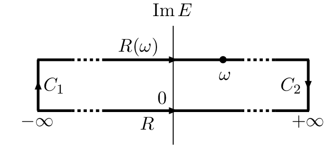
We can deform the contour of this EE integral along the real axis RR to the following:

R[−∞→+∞]⇒\displaystyle R[-\infty\rightarrow+\infty]\ \Rightarrow\ \phantom{+} C1[−∞+i0→−∞+iImω]\displaystyle C_{1}[-\infty+i0\rightarrow-\infty+i{\rm Im}\,\omega]
+\displaystyle{}+{} R(ω)[−∞+iImω→+∞+iImω]\displaystyle R(\omega)[-\infty+i{\rm Im}\,\omega\rightarrow+\infty+i{\rm Im}\,\omega]
+\displaystyle{}+{} C2[+∞+iImω→+∞+i0],\displaystyle C_{2}[+\infty+i{\rm Im}\,\omega\rightarrow+\infty+i0]\,, (53)

where the deformed contour is shown in Fig. 3. The integrals along the finite vertical segments C1C_{1} and C2C_{2} vanish since exp[−(E−ω)2/a2]\exp[-(E-\omega)^{2}/a^{2}] vanishes for Re​E→±∞{\rm Re}\,E\rightarrow\pm\infty with Im​E{\rm Im}\,E kept finite. The integral can thus be evaluated by the contour integral along R⁡(ω)R(\omega), which denotes the horizontal contour parallel to the real axis RR and passing the point z=ωz=\omega i.e., z=x+i​Im​ωz=x+i{\rm Im}\,\omega (with real x∈[−∞,∞]x\in[-\infty,\infty]). This deformation is allowed when the test function f⁡(E)f(E) is analytic in the complex plane inside the rectangular region surrounded by R+C1+R⁡(ω)+C2R+C_{1}+R(\omega)+C_{2} (see Fig. 3). The integral along R⁡(ω)R(\omega) is evaluated by making the change of variable E=E′+i​Im​ωE=E^{\prime}+i{\rm Im}\,\omega where E′E^{\prime} is real on R⁡(ω)R(\omega) and δc​(E−ω)\delta_{\rm c}(E-\omega) reduces to the usual Dirac’s delta δ⁡(E′−Re​ω)\delta(E^{\prime}-{\rm Re}\,\omega) since E−ω=E′−Re​ωE-\omega=E^{\prime}-{\rm Re}\,\omega is real on R⁡(ω)R(\omega). With this we find

∫R⁡(ω)d​E​δc​(E−ω)​f​(E)=∫−∞∞d​E′​δ​(E′−Re​ω)​f​(E′+i​Im​ω)=f⁡(Re​ω+i​Im​ω)=f⁡(ω),\int_{R(\omega)}dE\,\delta_{\rm c}(E-\omega)f(E)=\int_{-\infty}^{\infty}dE^{\prime}\,\delta(E^{\prime}-{\rm Re}\,\omega)f(E^{\prime}+i{\rm Im}\,\omega)=f({\rm Re}\,\omega+i{\rm Im}\,\omega)=f(\omega)\,, (54)

which proves that the distribution δc​(E−ω)\delta_{\rm c}(E-\omega) works as if it is the usual Dirac’s delta function despite the fact that EE is real and ω\omega is complex. This also proves

δc​(E−ω)​f​(E)=δc​(E−ω)​f​(ω),\delta_{\rm c}(E-\omega)f(E)=\delta_{\rm c}(E-\omega)f(\omega), (55)

which proves Eq. (42) when f⁡(E)=δc​(E−ω)f(E)=\delta_{\rm c}(E-\omega), as promised.

We should note that the remarkable property (54) for the complex delta function holds if and only if the test function f⁡(E)f(E) has no singularity inside the rectangular region stated above Nakanishi:1972wx. In practice however, f⁡(E)f(E) is usually given by the products of meromorphic Feynman propagators which often have pole singularities in the rectangular regions in question, in which case one has to pick up that contribution also. As we will see soon, this is actually the point touching the core of the problem.

In the actual scattering experiment, the total energy EE of the initial particles, P0=p10+p20P^{0}=p_{1}^{0}+p_{2}^{0}, must necessarily have a certain uncertainty around P0P^{0}, which may be described, for instance, by a Gaussian distribution with standard deviation σ\sigma of the form

fP0​(E)=12​π​σ2​exp⁡[−12​(E−P0σ)2].f_{P^{0}}(E)=\frac{1}{\sqrt{2\pi\sigma^{2}}}\exp\left[-\frac{1}{2}\Bigl(\frac{E-P^{0}}{\sigma}\Bigr)^{2}\right]\,. (56)

For such initial particles, the ghost production probability (44) should be averaged with this distribution. The actual production rate of complex ghost per unit space-time volume is then found to be

Pφ\displaystyle P_{\varphi} =−Re⁡[f2​2​π​∫−∞∞d​E​fP0​(E)​δc​(E−ω)​12​ω]\displaystyle=-{\rm Re}\,\Bigl[f^{2}2\pi\int_{-\infty}^{\infty}dE\,f_{P^{0}}(E)\delta_{\rm c}(E-\omega)\frac{1}{2\omega}\Bigr]
=−Re⁡[f2​πω​fP0​(ω)]=−f22​π​σ2​Re​[πω​exp⁡[−12​(ω−P0σ)2]],\displaystyle=-{\rm Re}\,\Bigl[f^{2}\frac{\pi}{\omega}f_{P^{0}}(\omega)\Bigr]=-\frac{f^{2}}{\sqrt{2\pi\sigma^{2}}}{\rm Re}\,\biggl[\frac{\pi}{\omega}\exp\Bigl[-\frac{1}{2}\Bigl(\frac{\omega-P^{0}}{\sigma}\Bigr)^{2}\Bigr]\biggr]\,, (57)

which is finite as far as σ\sigma is finite.

III.3 Imaginary part calculation of the forward scattering amplitude

Since the interaction Hamiltonian is hermitian, the total SS-matrix unitarity follows trivially and leads to the optical theorem for the TT-matrix:

S=1+(2​π)4​δ4​(PF−PI)​i​T^,\displaystyle S=1+(2\pi)^{4}\delta^{4}(P_{F}-P_{I})\,i\hat{T}\,,
S†S=1→2Im⟨I|T^|I⟩=(2π)4∑Fδ4(PF−PI)||T^|I⟩F||2,\displaystyle S^{\dagger}S=1\rightarrow 2{\rm Im}\,\left\langle{I}\right|\hat{T}\left|{I}\right\rangle=(2\pi)^{4}\sum_{F}\delta^{4}(P_{F}-P_{I})\,\big|\!\big|\,\hat{T}\left|{I}\right\rangle_{F}\big|\!\big|^{2}\,, (58)

where T^|I⟩F\hat{T}\left|{I}\right\rangle_{F} denotes all independent states |F⟩\left|{F}\right\rangle contained in the final scattered state T^|I⟩\hat{T}\left|{I}\right\rangle. In perturbation theory, this optical theorem holds for each set of the same order terms in the coupling constant ff. Additionally, the imaginary part of the particular Feynman diagram on the LHS equals the RHS with the sum over FF restricted to a certain subset.

Let us now calculate the forward scattering amplitude of two physical particles with the initial state |I(𝒑1,𝒑2)⟩\left|{I({\bm{p}}_{1},{\bm{p}}_{2})}\right\rangle in Eq. (33). At second order in ff of the interaction Lagrangian (32), there are only three diagrams which have ϕ\phi-propagator in ss-, tt- and uu-channels, and we calculate only the ss-channel amplitude since it has an imaginary part that reproduces the ϕ\phi-production probability in the previous subsection III.1. Here we note that the result Eq. (41) which we have found as the norm of the produced ϕ\phi-particle state (34) in the subsection III.1 can be rewritten in the form of the RHS of optical theorem (58) as

(2π)4∑𝒒δ4(PF−PI)||T^|I(𝒑1,𝒑2)⟩ϕ⁡(𝒒)-prod.||2\displaystyle(2\pi)^{4}\sum_{{\bm{q}}}\delta^{4}(P_{F}-P_{I})\big|\!\big|\,\hat{T}\left|{I({\bm{p}}_{1},{\bm{p}}_{2})}\right\rangle_{\text{$\phi({\bm{q}})$-prod.}}\big|\!\big|^{2}
=f2​∫d3​𝒒(2​π)3​(2​π)3​δ3​(𝒒−𝑷)​{2​π​δ​(ν𝒒−P0)​12​ν𝒒−Re⁡[2​π​δc​(ω𝒒−P0)​12​ω𝒒]}.\displaystyle=f^{2}\,\int\frac{d^{3}{\bm{q}}}{(2\pi)^{3}}(2\pi)^{3}\delta^{3}({\bm{q}}-{\bm{P}})\bigg\{2\pi\delta(\nu_{\bm{q}}-P^{0})\frac{1}{2\nu_{\bm{q}}}-{\rm Re}\,\Big[2\pi\delta_{\rm c}(\omega_{\bm{q}}-P^{0})\frac{1}{2\omega_{\bm{q}}}\Big]\bigg\}\,. (59)

We should find the same result by calculating the imaginary part of the forward scattering amplitude on the LHS of the optical theorem (58). The ss-channel tree level amplitude at O⁡(f2)O(f^{2}) corresponding to the Feynman diagram Fig. 2 (right) is now also easily computed:

⟨I′(𝒑1′,𝒑2′)|(S−1)|I(𝒑1,𝒑2)⟩|s-ch.(=i(2π)4δ4(P′−P)⟨I′(𝒑1′,𝒑2′)|T^|I(𝒑1,𝒑2)⟩|s-ch.)\displaystyle\left\langle{I^{\prime}({\bm{p}}^{\prime}_{1},{\bm{p}}^{\prime}_{2})}\right|(S-1)\left|{I({\bm{p}}_{1},{\bm{p}}_{2})}\right\rangle\big|_{\text{$s$-ch.}}\Bigl({}=i(2\pi)^{4}\delta^{4}(P^{\prime}-P)\left\langle{I^{\prime}({\bm{p}}^{\prime}_{1},{\bm{p}}^{\prime}_{2})}\right|\hat{T}\left|{I({\bm{p}}_{1},{\bm{p}}_{2})}\right\rangle\big|_{\text{$s$-ch.}}\Bigr)
=⟨I′(𝒑1′,𝒑2′)|12(i​f2)2T∫d4xd4yCa(x0)ψ2(x)ϕ(x)Ca(y0)ψ2(y)ϕ(y)|I(𝒑1,𝒑2)⟩|s-ch.\displaystyle\quad{}=\left\langle{I^{\prime}({\bm{p}}^{\prime}_{1},{\bm{p}}^{\prime}_{2})}\right|\frac{1}{2}\Big(\frac{if}{2}\Big)^{2}{\rm T}\int d^{4}x\,d^{4}y\,C_{a}(x^{0})\,\psi^{2}(x)\phi(x)\,C_{a}(y^{0})\psi^{2}(y)\phi(y)\left|{I({\bm{p}}_{1},{\bm{p}}_{2})}\right\rangle\big|_{\text{$s$-ch.}}
=(if)2∫d4xd4ye−i​P′​xCa(x0)⟨0|Tϕ(x)ϕ(y)|0⟩Ca(y0)ei​P​y,\displaystyle\quad{}=(if)^{2}\int d^{4}x\,d^{4}y\,e^{-iP^{\prime}x}C_{a}(x^{0})\left\langle{0}\right|{\rm T}\,\phi(x)\phi(y)\left|{0}\right\rangle\,C_{a}(y^{0})e^{iPy}\,, (60)

where Pμ:=p1μ+p2μ,P′μ:=p1′μ+p2′μP^{\mu}:=p_{1}^{\mu}+p_{2}^{\mu},P^{\prime\mu}:=p^{\prime\mu}_{1}+p^{\prime\mu}_{2} and Ca​(x)C_{a}(x) is the adiabatic Gaussian cutoff (37). We will compute this SS-matrix element (60) in two ways; first using the 3d-momentum form (29) of the ϕ\phi propagator, and second using the covariant 4d-momentum form (30). We will explicitly see why a careful treatment of a regularization (cutoff) (37) is indispensable for obtaining a coincident final result in both calculations. Once the equivalence of these methods is established, we can use either form of the propagator freely.

III.3.1 Use of 3d-momentum form of the ϕ\phi propagator

We first present the calculation using the 3d-momentum form (29) of the ϕ\phi propagator. Now, we insert the 3d-momentum form (29) into the propagator ⟨0|T​ϕ​(x)​ϕ​(y)|0⟩\left\langle{0|{\rm T}\phi(x)\phi(y)|0}\right\rangle in Eq. (60). Then, making a change of time variables (x0,y0)(x^{0},y^{0}) into CM and relative time (T,t)(T,t)

{T=12​(x0+y0)t=x0−y0→{x0=T+t/2y0=T−t/2,d​x0​d​y0=d​T​d​t\begin{cases}T=\frac{1}{2}(x^{0}+y^{0})\\ t=x^{0}-y^{0}\end{cases}\rightarrow\begin{cases}x^{0}=T+t/2\\ y^{0}=T-t/2\end{cases}\,,\quad dx^{0}dy^{0}=dTdt (61)

and writing explicitly the adiabatic (Gaussian) cutoff factor (37) at both interaction points x0x^{0} and y0y^{0},

Ca​(x0)​Ca​(y0)=exp⁡(−a2​(x02+y02))=exp⁡(−2​a2​T2−12​a2​t2),C_{a}(x^{0})C_{a}(y^{0})=\exp(-a^{2}({x^{0}}^{2}+{y^{0}}^{2}))=\exp\left(-2a^{2}T^{2}-\frac{1}{2}a^{2}t^{2}\right)\,, (62)

we have, after performing the d3​𝒙​d3​𝒚d^{3}{\bm{x}}d^{3}{\bm{y}} integrations and using δ3​(𝑷′−𝒒)​δ3​(𝒒−𝑷)=δ3​(𝑷′−𝑷)​δ3​(𝒒−𝑷)\delta^{3}({\bm{P}}^{\prime}-{\bm{q}})\delta^{3}({\bm{q}}-{\bm{P}})=\delta^{3}({\bm{P}}^{\prime}-{\bm{P}})\delta^{3}({\bm{q}}-{\bm{P}}),

LHS of (60)
=(i​f)2​∑aηa​(2​π)3​δ3​(𝑷′−𝑷)​∫d3​𝒒(2​π)3​2​ω𝒒a​(2​π)3​δ3​(𝒒−𝑷)\displaystyle\hskip 5.0pt=(if)^{2}\sum_{a}\eta_{a}(2\pi)^{3}\delta^{3}({\bm{P}}^{\prime}-{\bm{P}})\int\frac{d^{3}{\bm{q}}}{(2\pi)^{3}2{\omega}_{\bm{q}}^{a}}(2\pi)^{3}\delta^{3}({\bm{q}}-{\bm{P}})
×∫dTe−2​a2​T2ei⁡(P′0−P0)​T∫dte−a2t2/2(θ(t)ei⁡(P¯0−ω𝒒a)​t+θ(−t)ei⁡(P¯0+ω𝒒a)​t)\displaystyle\hskip 10.00002pt\times\int dT\,e^{-2a^{2}T^{2}}e^{i(P^{\prime 0}-P^{0})T}\int dt\,e^{-a^{2}t^{2}/2}\Bigl(\theta(t)e^{i(\overline{P}^{0}-{\omega}_{\bm{q}}^{a})t}+\theta(-t)e^{i(\overline{P}^{0}+{\omega}_{\bm{q}}^{a})t}\Bigr) (63)

with P¯0:=(P′0+P0)/2\overline{P}^{0}:=(P^{\prime 0}+P^{0})/2. Note that the integrations of the CM time TT and relative time tt are totally separated including their adiabatic cutoff factors. The d​TdT integration yields the factor

∫d​T​e−2​a2​T2​ei⁡(P′0−P0)​T=2​π​Δ2​a​(P′0−P0)​⟶a→0​(2​π)​δ​(P′0−P0),\int dT\,e^{-2a^{2}T^{2}}e^{i(P^{\prime 0}-P^{0})T}=2\pi\Delta_{\sqrt{2}a}(P^{\prime 0}-P^{0})\ \underset{a\rightarrow 0}{\longrightarrow}\ (2\pi)\delta(P^{\prime 0}-P^{0})\,, (64)

which together with the above (2​π)3​δ3​(𝑷′−𝑷)(2\pi)^{3}\delta^{3}({\bm{P}}^{\prime}-{\bm{P}}) completes the total energy-momentum conservation factor i​(2​π)4​δ4​(P′−P)i(2\pi)^{4}\delta^{4}(P^{\prime}-P), which should be divided out when giving a TT-matrix element.

Next, we consider the d​tdt integration part (denoting P¯0\bar{P}^{0} by EE as in (48))

∫dte−a2t2/2(θ(t)ei⁡(E−ω𝒒a)​t+θ(−t)ei⁡(E+ω𝒒a)​t).\displaystyle\int dt\,e^{-a^{2}t^{2}/2}\Big(\theta(t)e^{i(E-\omega^{a}_{\bm{q}})t}+\theta(-t)e^{i(E+\omega_{\bm{q}}^{a})t}\Big)\,. (65)

For the anti-ghost case first, ω𝒒a=ω𝒒∗\omega_{\bm{q}}^{a}=\omega^{*}_{\bm{q}} has negative imaginary part Im​ω𝒒∗<0{\rm Im}\,\omega_{\bm{q}}^{*}<0. We note that the integral converges even in the limit a→0a\rightarrow 0 since ei⁡(E∓ω𝒒∗)​te^{i(E\mp\omega^{*}_{\bm{q}})t} decreases exponentially as t→±∞t\rightarrow\pm\infty, meaning that the a→0a\rightarrow 0 limit is easily calculated by setting a=0a=0 from the beginning:

∫d​t​(θ⁡(t)​ei⁡(E−ω𝒒∗)​t+θ⁡(−t)​ei⁡(E+ω𝒒∗)​t)\displaystyle\int dt\,\Big(\theta(t)e^{i(E-\omega^{*}_{\bm{q}})t}+\theta(-t)e^{i(E+\omega^{*}_{\bm{q}})t}\Big) =[ei⁡(E−ω𝒒∗)​ti⁡(E−ω𝒒∗)]0∞+[ei⁡(E+ω𝒒∗)​ti⁡(E+ω𝒒∗)]−∞0\displaystyle=\left[\frac{e^{i(E-\omega^{*}_{\bm{q}})t}}{i(E-\omega^{*}_{\bm{q}})}\right]^{\infty}_{0}+\left[\frac{e^{i(E+\omega_{\bm{q}}^{*})t}}{i(E+\omega_{\bm{q}}^{*})}\right]^{0}_{-\infty}
=i⁡(1E−ω𝒒∗−1E+ω𝒒∗).\displaystyle=i\left(\frac{1}{E-\omega^{*}_{\bm{q}}}-\frac{1}{E+\omega_{\bm{q}}^{*}}\right)\,. (66)

In the ghost case, ω𝒒a=ω𝒒\omega_{\bm{q}}^{a}=\omega_{\bm{q}} has positive imaginary part Im​ω𝒒>0{\rm Im}\,\omega_{\bm{q}}>0 oppositely to the anti-ghost case. So the a→0a\rightarrow 0 limit is divergent since ei⁡(E∓ω𝒒)​te^{i(E\mp\omega_{\bm{q}})t} exponentially blows up as t→±∞t\rightarrow\pm\infty, respectively. But this also implies that the functions ei⁡(E∓ω𝒒)​te^{i(E\mp\omega_{\bm{q}})t} decrease exponentially in the opposite directions t→∓∞t\rightarrow\mp\infty. If we rewrite θ⁡(±t)\theta(\pm t) as 1−θ⁡(∓t)1-\theta(\mp t) in Eq. (65), then those terms with a −θ⁡(∓t)-\theta(\mp t) part give convergent quantities in the a→0a\rightarrow 0 limit as in the anti-ghost case, while the terms with 11 give the regularized complex delta function; that is, we can evaluate Eq. (65) in the ghost case as

lima→0∫dte−a2t2/2(θ(t)ei⁡(E−ω𝒒)​t+θ(−t)ei⁡(E+ω𝒒)​t)\displaystyle\lim_{a\rightarrow 0}\int dt\,e^{-a^{2}t^{2}/2}\Big(\theta(t)e^{i(E-\omega_{\bm{q}})t}+\theta(-t)e^{i(E+\omega_{\bm{q}})t}\Big)
=lima→0∫dte−a2t2/2(ei⁡(E−ω𝒒)​t+ei⁡(E+ω𝒒)​t)−∫dt(θ(−t)ei⁡(E−ω𝒒)​t+θ(+t)ei⁡(E+ω𝒒)​t)\displaystyle\ =\lim_{a\rightarrow 0}\int dt\,e^{-a^{2}t^{2}/2}\,\Big(e^{i(E-\omega_{\bm{q}})t}+e^{i(E+\omega_{\bm{q}})t}\Big)-\int dt\,\Big(\theta(-t)e^{i(E-\omega_{\bm{q}})t}+\theta(+t)e^{i(E+\omega_{\bm{q}})t}\Big)
=lima→0(2​π​Δa/2​(E−ω𝒒)+2​π​Δa/2​(E+ω𝒒))−[ei⁡(E−ω𝒒)​ti⁡(E−ω𝒒)]−∞0−[ei⁡(E+ω𝒒)​ti⁡(E+ω𝒒)]0+∞\displaystyle\ =\lim_{a\rightarrow 0}\left(2\pi\Delta_{a/\sqrt{2}}(E-\omega_{\bm{q}})+2\pi\Delta_{a/\sqrt{2}}(E+\omega_{\bm{q}})\right)-\left[\frac{e^{i(E-\omega_{\bm{q}})t}}{i(E-\omega_{\bm{q}})}\right]^{0}_{-\infty}-\left[\frac{e^{i(E+\omega_{\bm{q}})t}}{i(E+\omega_{\bm{q}})}\right]_{0}^{+\infty}
=2​π​δc​(E−ω𝒒)+2​π​δc​(E+ω𝒒)+i⁡(1E−ω𝒒−1E+ω𝒒).\displaystyle\ =2\pi\delta_{\rm c}(E-\omega_{\bm{q}})+2\pi\delta_{\rm c}(E+\omega_{\bm{q}})+i\left(\frac{1}{E-\omega_{\bm{q}}}-\frac{1}{E+\omega_{\bm{q}}}\right)\,. (67)

Finally, we consider the ‘photon’ which has a real energy ω𝒒a=ν𝒒\omega_{\bm{q}}^{a}=\nu_{\bm{q}}. In this case, we can follow the usual −i​ε-i\varepsilon trick to shift the mass square which results in the energy shift ν𝒒→ν𝒒−i​ε\nu_{\bm{q}}\rightarrow\nu_{\bm{q}}-i\varepsilon. Then, since Im⁡(ν𝒒−i​ε)<0{\rm Im}\,(\nu_{\bm{q}}-i\varepsilon)<0, this reduces to the above anti-ghost case and the result (66) immediately gives

∫d​t​(θ⁡(t)​ei⁡(E−ν𝒒+i​ε)​t+θ⁡(−t)​ei⁡(E+ν𝒒−i​ε)​t)\displaystyle\int dt\,\Big(\theta(t)e^{i(E-\nu_{\bm{q}}+i\varepsilon)t}+\theta(-t)e^{i(E+\nu_{\bm{q}}-i\varepsilon)t}\Big) =i⁡(1E−ν𝒒+i​ε−1E+ν𝒒−i​ε).\displaystyle=i\left(\frac{1}{E-\nu_{\bm{q}}+i\varepsilon}-\frac{1}{E+\nu_{\bm{q}}-i\varepsilon}\right)\,. (68)

If we recall the well-known formula 1/(x∓i​ε)=P⁡(1/x)±i​π​δ​(x)1/(x\mp i\varepsilon)={\rm P}(1/x)\pm i\pi\delta(x) (with P{\rm P} denoting principal value), this result can be rewritten into the form

Eq. (68)=i​P​(1E−ν𝒒)−i​P​(1E+ν𝒒)+π​δ​(E−ν𝒒)+π​δ​(E+ν𝒒).\hbox{Eq.~(\ref{ImOmega=0})}=i{\rm P}\Big(\frac{1}{E-\nu_{\bm{q}}}\Big)-i{\rm P}\Big(\frac{1}{E+\nu_{\bm{q}}}\Big)+\pi\delta(E-\nu_{\bm{q}})+\pi\delta(E+\nu_{\bm{q}})\,. (69)

It is interesting to note that this can further be rewritten into

=i⁡(1E−ν𝒒−i​ε−1E+ν𝒒+i​ε)+2​π​δ​(E−ν𝒒)+2​π​δ​(E+ν𝒒),=i\left(\frac{1}{E-\nu_{\bm{q}}-i\varepsilon}-\frac{1}{E+\nu_{\bm{q}}+i\varepsilon}\right)+2\pi\delta(E-\nu_{\bm{q}})+2\pi\delta(E+\nu_{\bm{q}})\,, (70)

which is the same result as the one which we would have obtained if we had used +i​ε+i\varepsilon trick to replace ν𝒒→ν𝒒+i​ε\nu_{\bm{q}}\rightarrow\nu_{\bm{q}}+i\varepsilon and applied the formula (67) for the ghost case. Since (68) equals (70), both tricks replacing ν𝒒\nu_{\bm{q}} by ν𝒒±i​ε\nu_{\bm{q}}\pm i\varepsilon lead to the same result.

Now, let us go back to the Eq. (63). We apply these formulas (68), (67) and (66) to the d​tdt integration part (65) for ϕa=\phi_{a}= ‘photon’ AA,  ghost φ\varphi and anti-ghost φ†\varphi^{\dagger}, respectively, and divide out the total energy-momentum conservation factor i​(2​π)4​δ4​(P′−P)i(2\pi)^{4}\delta^{4}(P^{\prime}-P), setting P=P′P=P^{\prime} in the Eq. (63), to find the forward scattering transition amplitude

⟨I|T^|I⟩|s-ch.\displaystyle\left\langle{I}\right|\hat{T}\left|{I}\right\rangle\big|_{\text{$s$-ch.}}
=f2∫d3𝒒δ3(𝒒−𝑷)[−12​ν𝒒(1P0−ν𝒒+i​ε−1P0+ν𝒒−i​ε)\displaystyle=f^{2}\int d^{3}{\bm{q}}\,\delta^{3}({\bm{q}}-{\bm{P}})\biggl[-\frac{1}{2\nu_{\bm{q}}}\Big(\frac{1}{P^{0}-\nu_{\bm{q}}+i\varepsilon}-\frac{1}{P^{0}+\nu_{\bm{q}}-i\varepsilon}\Big)
−12(1−P02+𝒒2+M2+i2​π2​ω𝒒(δc(P0−ω𝒒)+δc(P0+ω𝒒))+1−P02+𝒒2+M∗2)]\displaystyle\hskip 15.00002pt{}-\frac{1}{2}\left(\frac{1}{-{P^{0}}^{2}+{\bm{q}}^{2}+M^{2}}+i\frac{2\pi}{2\omega_{\bm{q}}}\left(\delta_{\rm c}(P^{0}-\omega_{{\bm{q}}})+\delta_{\rm c}(P^{0}+\omega_{{\bm{q}}})\right)+\frac{1}{-{P^{0}}^{2}+{\bm{q}}^{2}+{M^{*}}^{2}}\right)\biggr]
=f2​[1P2+δ2−i​ε−12​(1P2+M2+1P2+M∗2)−i​π2​ω𝑷​(δc​(P0−ω𝑷)+δc​(P0+ω𝑷))],\displaystyle=f^{2}\biggl[\frac{1}{P^{2}+\delta^{2}-i\varepsilon}-\frac{1}{2}\Bigl(\frac{1}{P^{2}+M^{2}}+\frac{1}{P^{2}+{M^{*}}^{2}}\Bigr)-i\frac{\pi}{2\omega_{\bm{P}}}\Bigl(\delta_{\rm c}(P^{0}-\omega_{\bm{P}})+\delta_{\rm c}(P^{0}+\omega_{\bm{P}})\Bigr)\biggr]\,, (71)

where we have used −P02+ω𝒒a2=−P02+𝒒2+ma2=P2+ma2-{P_{0}}^{2}+{\omega^{a}_{\bm{q}}}^{2}=-P_{0}^{2}+{\bm{q}}^{2}+m_{a}^{2}=P^{2}+m_{a}^{2} with ma2=(δ2,M2,M∗2)m_{a}^{2}=(\delta^{2},M^{2},{M^{*}}^{2}) in the presence of δ3​(𝑷−𝒒)\delta^{3}({\bm{P}}-{\bm{q}}). We thus finally obtain the imaginary part of the ss-channel forward transition amplitude,

2Im⟨I|T^|I⟩|s-ch.=f2[πν𝑷δ(P0−ν𝑷)−Re[πω𝑷δc(P0−ω𝑷)]],2{\rm Im}\,\,\left\langle{I}\right|\hat{T}\left|{I}\right\rangle\big|_{\text{$s$-ch.}}=f^{2}\bigg[\frac{\pi}{\nu_{\bm{P}}}\,\delta(P^{0}-\nu_{\bm{P}})-{\rm Re}\,\Big[\frac{\pi}{\omega_{\bm{P}}}\,\delta_{\rm c}(P^{0}-\omega_{\bm{P}})\Big]\bigg]\,, (72)

where we have omitted the terms δ⁡(P0+ν𝑷)\delta(P^{0}+\nu_{\bm{P}}) and δc​(P0+ω𝑷)\delta_{\rm c}(P^{0}+\omega_{\bm{P}}) since they vanish for P0>0P^{0}>0.1010 10 This is because the complex delta function δc​(P0+ω𝑷)\delta_{\rm c}(P^{0}+\omega_{\bm{P}}) has non-vanishing support only within −Re​ω𝑷−Im​ω𝑷≤P0≤−Re​ω𝑷+Im​ω𝑷-{\rm Re}\,\omega_{\bm{P}}-{\rm Im}\,\omega_{\bm{P}}\leq P^{0}\leq-{\rm Re}\,\omega_{\bm{P}}+{\rm Im}\,\omega_{\bm{P}}, but we have Im​ω𝟎<Re​ω𝟎{\rm Im}\,\omega_{\bf 0}<{\rm Re}\,\omega_{\bf 0} for Re​M2>0{\rm Re}\,M^{2}>0 and Im​M2>0{\rm Im}\,M^{2}>0 which leads to Im​ω𝑷<Re​ω𝑷{\rm Im}\,\omega_{{\bm{P}}}<{\rm Re}\,\omega_{{\bm{P}}}, implying −Re​ω𝑷−Im​ω𝑷≤P0≤−Re​ω𝑷+Im​ω𝑷<0-{\rm Re}\,\omega_{\bm{P}}-{\rm Im}\,\omega_{\bm{P}}\leq P^{0}\leq-{\rm Re}\,\omega_{\bm{P}}+{\rm Im}\,\omega_{\bm{P}}<0. This imaginary part exactly coincides with the RHS result (41) divided by (2​π)4​δ4​(0)(2\pi)^{4}\delta^{4}(0), that gives the ϕ\phi-production rate per unit space-time volume directly calculated in the previous subsection III.1, thus confirming the optical theorem (58).

III.3.2 Use of 4d-momentum form of the ϕ\phi propagator

Now we present the calculation of the SS-matrix element (60) using the 4d-momentum form (30) of the propagator:

⟨I′(𝒑1′,𝒑2′)|(S−1)|I(𝒑1,𝒑2)⟩|s-ch.\displaystyle\left\langle{I^{\prime}({\bm{p}}^{\prime}_{1},{\bm{p}}^{\prime}_{2})}\right|(S-1)\left|{I({\bm{p}}_{1},{\bm{p}}_{2})}\right\rangle\big|_{\text{$s$-ch.}}
=(i​f)2​∫d4​x​d4​y​e−i​P′​x+i​P​y\displaystyle\quad{}=(if)^{2}\int d^{4}x\,d^{4}y\,e^{-iP^{\prime}x+iPy}
×∫d3​𝒒i​(2​π)4​[∫Rd​q0q2+δ2−12​(∫Cd​q0q2+M2+∫Rd​q0q2+M∗2)]​ei​q​(x−y),\displaystyle\qquad\times\int{d^{3}{\bm{q}}\over i(2\pi)^{4}}\left[\int_{R}\frac{dq^{0}}{q^{2}+\delta^{2}}-\frac{1}{2}\bigg(\int_{C}\frac{dq^{0}}{q^{2}+M^{2}}+\int_{R}\frac{dq^{0}}{q^{2}+{M^{*}}^{2}}\bigg)\right]\,e^{iq(x-y)}, (73)

where we recall that the q0q^{0}-integration contour for the ghost φ\varphi is the much deformed CC drawn in Fig. 1 (left), while those for ‘photon’ AA and anti-ghost φ†\varphi^{\dagger} are along the real axis RR. Then, performing the d4​xd^{4}x and d4​yd^{4}y integrations yields 1111 11 Note that the delta functions appearing here are generally complex delta functions, but the usual manipulation extracting the total energy-momentum conservation factor (2​π)4​δ4​(P′−P)(2\pi)^{4}\delta^{4}(P^{\prime}-P) is possible as shown in the equation here and explained in the previous subsection.

(2​π)4​δc4​(P′−q)⋅(2​π)4​δc4​(q−P)=(2​π)4​δ4​(P′−P)⋅(2​π)4​δc4​(q−P),(2\pi)^{4}\delta_{\rm c}^{4}(P^{\prime}-q)\cdot(2\pi)^{4}\delta_{\rm c}^{4}(q-P)=(2\pi)^{4}\delta^{4}(P^{\prime}-P)\cdot(2\pi)^{4}\delta_{\rm c}^{4}(q-P)\,, (74)

and after dividing out (ii times) the total momentum conservation factor, i​(2​π)4​δ4​(P′−P)i(2\pi)^{4}\delta^{4}(P^{\prime}-P), and setting P′=PP^{\prime}=P, we find the following expression for the TT-matrix element for the forward scattering ss-channel diagram:

⟨I|T^|I⟩|s-ch.=f2[∫Rd4​qq2+δ2−i​ε−12(∫Cd4​qq2+M2+∫Rd4​qq2+M∗2)]δc4(q−P).\displaystyle\left\langle{I}\right|\hat{T}\left|{I}\right\rangle\big|_{\text{$s$-ch.}}=f^{2}\left[\int_{R}\frac{d^{4}q}{q^{2}+\delta^{2}-i\varepsilon}-\frac{1}{2}\bigg(\int_{C}\frac{d^{4}q}{q^{2}+M^{2}}\!+\!\int_{R}\frac{d^{4}q}{q^{2}+{M^{*}}^{2}}\bigg)\right]\delta^{4}_{\rm c}(q-P)\,. (75)

Suppose that we perform the d4​qd^{4}q integrations in this Eq. (75) to simply put qμq^{\mu} equal to PμP^{\mu} by naively using the complex delta function δc​(q−P)\delta_{\rm c}(q-P), as if it were just like the Dirac delta function. We would then immediately obtain 1212 12 The sum of the ghost and anti-ghost propagators in (76) is the real propagator for the fakeon Anselmi:2017ygm; Anselmi:2018kgz.

⟨I|T^|I⟩|s-ch.=?f2[1P2+δ2−i​ε−12(1P2+M2+1P2+M∗2)],\left\langle{I}\right|\hat{T}\left|{I}\right\rangle\big|_{\text{$s$-ch.}}\ \overset{?}{=}\ f^{2}\left[\frac{1}{P^{2}+\delta^{2}-i\varepsilon}-\frac{1}{2}\bigg(\frac{1}{P^{2}+M^{2}}+\frac{1}{P^{2}+{M^{*}}^{2}}\bigg)\right]\,, (76)

which is exactly the expression that one would write down if the usual Feynman rule in momentum space is applied directly to the diagram Fig. 2 (right), in which the naive energy-momentum conservation at each vertex is tacitly assumed in advance. This represents a very elementary, but very serious mistake which many have made, including Lee and Wick, and even many of those who were critical of their theory for other reasons. If Eq. (76) were correct, the ghost contributions, the second and third terms, add up to a real quantity and thus do not contribute to the imaginary part of the transition amplitude. Only the first ‘photon’ part gives the following imaginary part (for the ss-channel P0>0P^{0}>0):

2Im⟨I|T^|I⟩|s-ch.\displaystyle 2{\rm Im}\,\,\left\langle{I}\right|\hat{T}\left|{I}\right\rangle\big|_{\text{$s$-ch.}} =\displaystyle= f2​πν𝑷​δ​(P0−ν𝑷),\displaystyle f^{2}\frac{\pi}{\nu_{\bm{P}}}\delta(P^{0}-\nu_{\bm{P}})\,, (77)

where the term proportional to δ⁡(P0+ν𝑷)=0\delta(P^{0}+\nu_{\bm{P}})=0 is suppressed. Essentially by this type of calculation and reasoning, Lee and Wick concluded that the complex ghosts are not produced from physical particle scattering.

The correct computation of the RHS of Eq. (75) should be performed as follows, noting that the naive use of the complex delta function δc​(q0−P0)\delta_{\rm c}(q^{0}-P^{0}) is allowed when the integration variable q0q^{0} remains real all the way along the contour since then δc​(q0−P0)\delta_{\rm c}(q^{0}-P^{0}) is reduced to the usual Dirac delta function δ⁡(q0−P0)\delta(q^{0}-P^{0}) with real argument q0−P0q^{0}-P^{0}. Since this is already the case for the first term (‘photon’ part) and the third term (anti-ghost part), the problem lies in the second term (ghost part), for which the integration contour CC is much deformed one as depicted in Fig. 1 (left) on the complex q0q^{0} plane. To avoid the moving imaginary part Im​q0{\rm Im}\,q^{0} on CC, we can deform the contour CC according to

∫Cdq0→(∫R+∫C⁡(−ω𝒒)−∫C⁡(+ω𝒒))dq0,\int_{C}dq^{0}\ \rightarrow\ \bigg(\int_{R}+\int_{C(-\omega_{\bm{q}})}-\int_{C(+\omega_{\bm{q}})}\bigg)dq^{0}\,, (78)

as shown in Fig. 1 (right), where C⁡(ω)C(\omega) denotes an infinitesimal circle rotating anti-clockwise around the pole at q0=ωq^{0}=\omega. Then, the first integral part ∫Rd​q0\int_{R}dq^{0} is again along the real axis, for which we can use the naive substitution rule q0→P0q^{0}\rightarrow P^{0} also for the second term (ghost part). This contribution together with those from the first and third terms in (75) reproduces Lee and Wick’s amplitude (76), which results from applying the usual Feynman rule with energy-momentum conservation assumed at each vertex.

Here, however, we have two extra contributions from the two circles C⁡(±ω𝒒)C(\pm\omega_{\bm{q}}) which can be evaluated by the pole residues according to Cauchy’s theorem:1313 13 It is important to note that the complex delta function δc​(q0−P0)\delta_{\rm c}(q^{0}-P^{0}) is the a→0a\rightarrow 0 limit of the analytic (Gaussian) function Δa​(q0−P0)\Delta_{a}(q^{0}-P^{0}) which has no singularity in the relevant domain for the deformation performed in Eq. (78).

−\displaystyle- f22∫d3𝒒δ3(𝒒−𝑷)(∫C⁡(−ω𝒒)−∫C⁡(+ω𝒒))dq01−q02+ω𝒒2δc(q0−P0)\displaystyle\frac{f^{2}}{2}\int d^{3}{\bm{q}}\,\delta^{3}({\bm{q}}-{\bm{P}})\bigg(\int_{C(-\omega_{\bm{q}})}-\int_{C(+\omega_{\bm{q}})}\bigg)dq^{0}\frac{1}{-{q^{0}}^{2}+\omega^{2}_{\bm{q}}}\delta_{\rm c}(q^{0}-P^{0})
=−f22∫d3𝒒δ3(𝒒−𝑷)(2​π​i2​ω𝒒(δc(ω𝒒−P0)+δc(−ω𝒒−P0)))\displaystyle=-\frac{f^{2}}{2}\int d^{3}{\bm{q}}\,\delta^{3}({\bm{q}}-{\bm{P}})\bigg(\frac{2\pi i}{2\omega_{\bm{q}}}\Bigl(\delta_{\rm c}(\omega_{\bm{q}}-P^{0})+\delta_{\rm c}(-\omega_{\bm{q}}-P^{0})\Bigr)\bigg)
=−f2​i​π2​ω𝑷​(δc​(P0−ω𝑷)+δc​(P0+ω𝑷)).\displaystyle=-f^{2}\frac{i\pi}{2\omega_{\bm{P}}}\Bigl(\delta_{\rm c}(P^{0}-\omega_{\bm{P}})+\delta_{\rm c}(P^{0}+\omega_{\bm{P}})\Bigr)\,. (79)

Adding this to the Lee-Wick’s amplitude (76), exactly reproduces the previous result (71) obtained by using the 3d-momentum propagators.

At this stage we emphasize that in the 3d form of the propagators (27), the time propagation of the positive and negative energy components are clearly distinguished thanks to θ⁡(±t)\theta(\pm t) function, where, in the case of the ghost, we mean a positive or negative energy with respect to its real part. As a result, there is no violation of causality even in the presence of the ghost. However, the amplitude (76) will violate causality Coleman:1969xz; Donoghue:2019fcb; Donoghue:2021eto (see also Lee:1969fy), because the integration contour of the 4d form of the ghost and anti-ghost propagators (which inherits the causal information from the 3d form of the propagators) is completely ignored.

Refer to caption
Refer to caption
Figure 4: Left: Graphical presentation of the norm (104). Right: The one-loop amplitude for ψ+ψ→ψ+ψ\psi+\psi\rightarrow\psi+\psi

IV Ghost pair production

The one-loop amplitude for ψ+ψ→ψ+ψ\psi+\psi\rightarrow\psi+\psi shown in Fig. 4 (right) has been representatively considered to demonstrate the Lee-Wick prescription Lee:1969fy; Lee:1969zze; Lee:1970iw of how to integrate the loop momenta. According to their prescription, the imaginary part of the amplitude should vanish for the parts where ghost and/or anti-ghost are propagating in the loop. The optical theorem would then imply that the production of two ghost particles by a collision of two physical particles, i.e. ψ+ψ→B+B\psi+\psi\rightarrow B+B (B=(φ+φ†)/2B=(\varphi+\varphi^{\dagger})/\sqrt{2}) is forbidden. Here in this section we will examine their calculation in our field theory framework. To this end, we consider the interaction Lagrangian

ℒint​(ψ,ϕ)=−f2​ψ2​ϕ2.{\cal L}_{\rm int}(\psi,\phi)=-\frac{f}{2}\,\psi^{2}\phi^{2}\,. (80)

IV.1 Imaginary part calculation of the forward scattering amplitude

IV.1.1 Use of 3d-momentum form for the ϕ\phi propagator

Since we are interested in ghost production, we focus only on the ss-channel contribution to the one-loop amplitude for the scattering ψ+ψ→ψ+ψ\psi+\psi\rightarrow\psi+\psi. With the interaction Lagrangian ℒint{\cal L}_{\rm int} of (80), the calculation proceeds quite in parallel to that in the previous section. As in Eq. (60), we have at second order in the coupling ff

⟨I′(𝒑1′,𝒑2′)|(S−1)|I(𝒑1,𝒑2)⟩|s-ch.(=i(2π)4δ4(P′−P)⟨I′(𝒑1′,𝒑2′)|T^|I(𝒑1,𝒑2)⟩|s-ch.)\displaystyle\left\langle{I^{\prime}({\bm{p}}^{\prime}_{1},{\bm{p}}^{\prime}_{2})}\right|(S-1)\left|{I({\bm{p}}_{1},{\bm{p}}_{2})}\right\rangle\big|_{\text{$s$-ch.}}\Bigl({}=i(2\pi)^{4}\delta^{4}(P^{\prime}-P)\left\langle{I^{\prime}({\bm{p}}^{\prime}_{1},{\bm{p}}^{\prime}_{2})}\right|\hat{T}\left|{I({\bm{p}}_{1},{\bm{p}}_{2})}\right\rangle\big|_{\text{$s$-ch.}}\Bigr)
=⟨I′(𝒑1′,𝒑2′)|12(−i​f2)2T∫d4xd4yCa(x0)Ca(y0)ψ2(x)ϕ2(x)ψ2(y)ϕ2(y)|I(𝒑1,𝒑2)⟩|s-ch.\displaystyle\quad{}=\left\langle{I^{\prime}({\bm{p}}^{\prime}_{1},{\bm{p}}^{\prime}_{2})}\right|\frac{1}{2}\Big(\frac{-if}{2}\Big)^{2}{\rm T}\int d^{4}x\,d^{4}y\,C_{a}(x^{0})C_{a}(y^{0})\,\psi^{2}(x)\phi^{2}(x)\,\psi^{2}(y)\phi^{2}(y)\left|{I({\bm{p}}_{1},{\bm{p}}_{2})}\right\rangle\big|_{\text{$s$-ch.}}
=(i​f)2​∫d4​x​d4​y​e−i​P′​x+i​P​y​e−a2​(x0)2−a2​(y0)2​Σ​(x−y),\displaystyle\quad{}=(if)^{2}\int d^{4}x\,d^{4}y\,e^{-iP^{\prime}x+iPy}\,e^{-a^{2}(x^{0})^{2}-a^{2}(y^{0})^{2}}\,\Sigma(x-y)\,, (81)

with the initial 2​ψ2\psi state |I(𝒑1,𝒑2)⟩\left|{I({\bm{p}}_{1},{\bm{p}}_{2})}\right\rangle defined in (33) and P=p1+p2,P′=p1′+p2′P=p_{1}+p_{2}\,,P^{\prime}=p^{\prime}_{1}+p^{\prime}_{2}, where Ca​(x0)C_{a}(x^{0}) is the adiabatic cutoff introduced in Eq. (37) and Σ⁡(x−y)\Sigma(x-y) is given by

Σ⁡(x−y)\displaystyle\Sigma(x-y) :=2⟨0|Tϕ(x)ϕ(y)|0⟩2=2∑a,b=13ηaηbΣa​b(x−y),\displaystyle:=2\left\langle{0}\right|{\rm T}\,\phi(x)\phi(y)\left|{0}\right\rangle^{2}=2\sum_{a,b=1}^{3}\eta_{a}\eta_{b}\Sigma_{ab}(x-y)\,,
Σa​b​(x−y)\displaystyle\Sigma_{ab}(x-y) =(−1)|a|+|b|⟨0|Tϕa(x)ϕa(y)|0⟩⟨0|Tϕb(x)ϕb(y)|0⟩.\displaystyle=(-1)^{|a|+|b|}\left\langle{0}\right|{\rm T}\,\phi_{a}(x)\phi_{a}(y)\left|{0}\right\rangle\left\langle{0}\right|{\rm T}\,\phi_{b}(x)\phi_{b}(y)\left|{0}\right\rangle\,. (82)

Here, ϕa=(A,φ,φ†)\phi_{a}=(A,\,\varphi,\,\varphi^{\dagger}) are the three component fields in ϕ=A+(φ+φ†)/2\phi=A+(\varphi+\varphi^{\dagger})/\sqrt{2} with the weight factor ηa=(1,−1/2,−1/2)\eta_{a}=(1,\,-1/2,\,-1/2) and norm sign (−1)|a|=(+1,−1,−1)(-1)^{|a|}=(+1,\,-1,\,-1). Inserting the 3d momentum expression in Eq. (29) for the propagator ⟨0|Tϕa(x)ϕa(y)|0⟩\left\langle{0}\right|{\rm T}\,\phi_{a}(x)\phi_{a}(y)\left|{0}\right\rangle, we find a compact form for Σa​b\Sigma_{ab}:

Σa​b​(x−y)\displaystyle\Sigma_{ab}(x-y) =∫d3​𝒒​d3​𝒒′(2​π)6​2​ω𝒒a​2​ω𝒒′b​(θ⁡(x0−y0)​ei⁡(q^a+q^b′)​(x−y)+θ⁡(y0−x0)​e−i⁡(q^a+q^b′)​(x−y)),\displaystyle=\int\frac{d^{3}{\bm{q}}\,d^{3}{\bm{q}}^{\prime}}{(2\pi)^{6}2{\omega}^{a}_{\bm{q}}2{\omega}^{b}_{{\bm{q}}^{\prime}}}\Big(\theta(x^{0}-y^{0})e^{i(\widehat{q}_{a}+\widehat{q}^{\prime}_{b})(x-y)}+\theta(y^{0}-x^{0})e^{-i(\widehat{q}_{a}+\widehat{q}^{\prime}_{b})(x-y)}\Big)\,\,, (83)

where ω𝒒a{\omega}^{a}_{\bm{q}} and q^aμ\widehat{q}_{a}^{\mu} are the energy and the on-shell 4-momentum of ϕa\phi_{a} defined before in Eq. (31).

Noting the similarity between Eqs. (60) and (81), and recalling the procedure to obtain Eq. (63), we perform the d3​𝒙​d3​𝒚d^{3}{\bm{x}}d^{3}{\bm{y}} integrations in (81), yielding three dimensional delta functions (2​π)3​δ3​(𝒒+𝒒′−𝑷)(2\pi)^{3}\delta^{3}({\bm{q}}+{\bm{q}}^{\prime}-{\bm{P}}) and (2​π)3​δ3​(𝒒+𝒒′−𝑷′)(2\pi)^{3}\delta^{3}({\bm{q}}+{\bm{q}}^{\prime}-{\bm{P}}^{\prime}). This then allows us to carry out the integration over 𝒒′{\bm{q}}^{\prime} to write 𝒒′=−𝒒+𝑷=−𝒒+𝑷′{\bm{q}}^{\prime}=-{\bm{q}}+{\bm{P}}=-{\bm{q}}+{\bm{P}}^{\prime}. 1414 14 The second term in (83), i.e., the one proportional to θ⁡(−t)\theta(-t), actually gives 𝒒′=−𝒒−𝑷=−𝒒−𝑷′{\bm{q}}^{\prime}=-{\bm{q}}-{\bm{P}}=-{\bm{q}}-{\bm{P}}^{\prime}, but we make the change 𝒒→−𝒒{\bm{q}}\to-{\bm{q}} which implies −𝒒−𝑷→𝒒−𝑷-{\bm{q}}-{\bm{P}}\to{\bm{q}}-{\bm{P}}. We then use the fact that ν𝒒=ν−𝒒\nu_{{\bm{q}}}=\nu_{-{\bm{q}}} and ω𝒒=ω−𝒒\omega_{{\bm{q}}}=\omega_{-{\bm{q}}}. Then, as we have done in (61), we use the CM and relative time (T=(x0+y0)/2,t=x0−y0)(T=(x^{0}+y^{0})/2,\ t=x^{0}-y^{0}) to perform the time integration and obtain

⟨I′(𝒑1′,𝒑2′)|(S−1)|I(𝒑1,𝒑2)⟩|s-ch.\displaystyle\left\langle{I^{\prime}({\bm{p}}^{\prime}_{1},{\bm{p}}^{\prime}_{2})}\right|(S-1)\left|{I({\bm{p}}_{1},{\bm{p}}_{2})}\right\rangle\big|_{\text{$s$-ch.}}
=−f2​(2​π)3​δ3​(𝑷−𝑷′)​(∫d​T​ei⁡(P0−P′0)​T​e−2​a2​T2)\displaystyle=-f^{2}(2\pi)^{3}\delta^{3}({\bm{P}}-{\bm{P}}^{\prime})\Big(\int dT\,e^{i(P^{0}-P^{\prime 0})T}e^{-2a^{2}T^{2}}\Big)\,
×∫d3​𝒒(2​π)3∑a,b2​ηa​ηb2​ω𝒒a​ 2​ω𝑷−𝒒b∫dte−a2t2/2{θ(t)ei⁡(P0¯−q¯a​b0)​t+θ(−t)ei⁡(P0¯+q¯a​b0)​t},\displaystyle\times\int\frac{d^{3}{\bm{q}}}{(2\pi)^{3}}\,\sum_{a,b}\frac{2\eta_{a}\eta_{b}}{2{\omega}^{a}_{\bm{q}}\,2{\omega}^{b}_{{\bm{P}}-{\bm{q}}}}\int dt\,e^{-a^{2}t^{2}/2}\left\{\theta(t)\,e^{i(\bar{P^{0}}-\bar{q}^{0}_{ab})t}+\theta(-t)\,e^{i(\bar{P^{0}}+\bar{q}^{0}_{ab})t}\right\}\,, (84)

where P0¯=(P0+P′0)/2=(p10+p20+p1′0+p2′0)/2\bar{P^{0}}=(P^{0}+P^{\prime 0})/2=(p^{0}_{1}+p^{0}_{2}+p^{\prime 0}_{1}+p^{\prime 0}_{2})/2 and q¯a​b0=ω𝒒a+ω𝑷−𝒒b\bar{q}^{0}_{ab}=\omega^{a}_{\bm{q}}+\omega^{b}_{{\bm{P}}-{\bm{q}}}, and the TT integration gives (2​π)​δ​(P0−P′0)(2\pi)\delta(P^{0}-P^{\prime 0}) in the a→0a\to 0 limit. When applying the formulas to carry out the tt integration with either (67), (66), or (68) and θ⁡(±t)\theta(\pm t), we must classify the cases when the imaginary part of q¯a​b0=ω𝒒a+ω𝑷−𝒒b\bar{q}^{0}_{ab}=\omega^{a}_{\bm{q}}+\omega^{b}_{{\bm{P}}-{\bm{q}}} becomes positive or negative, which is a bit complicated task. In order to avoid such an inessential complication for the present issue of ghost production, we discuss the problem in the CM frame and set 𝑷=𝟎{\bm{P}}={\bf 0} henceforth. Then, the equality ω𝑷−𝒒a=ω𝒒a\omega^{a}_{{\bm{P}}-{\bm{q}}}=\omega^{a}_{\bm{q}} holds so that we have

Im​q¯a​b0=Im⁡(ω𝒒a+ω𝒒b)(ϕa,ϕb)​ or ​(ϕb,ϕa)Applied formulaIm​q¯a​b0=0:(A,A),(φ,φ†)Eq.​(68)Im​q¯a​b0>0:(A,φ),(φ,φ)Eq.​(67)Im​q¯a​b0<0:(A,φ†),(φ†,φ†)Eq.​(66).\begin{array}[]{cccl}{\rm Im}\,\bar{q}^{0}_{ab}={\rm Im}\,(\omega_{\bm{q}}^{a}+\omega_{\bm{q}}^{b})&&(\phi_{a},\,\phi_{b})\hbox{\ or\ }(\phi_{b},\,\phi_{a})&\text{Applied formula}\\ \hline\cr{\rm Im}\,\bar{q}^{0}_{ab}=0&:&(A,\,A),\ (\varphi,\,\varphi^{\dagger})&~~~\text{Eq.}(\ref{ImOmega=0})\\ {\rm Im}\,\bar{q}^{0}_{ab}>0&:&(A,\,\varphi),\ (\varphi,\,\varphi)&~~~\text{Eq.}(\ref{ImOmega>0})\\ {\rm Im}\,\bar{q}^{0}_{ab}<0&:&(A,\,\varphi^{\dagger}),\ (\varphi^{\dagger},\,\varphi^{\dagger})&~~~\text{Eq.}(\ref{ImOmega<0})\,.\end{array} (85)

Applying the indicated formula for the d​tdt integrations in (81), dividing out the factor i​(2​π)4​δ4​(P′−P)i(2\pi)^{4}\delta^{4}(P^{\prime}-P) and setting P=P′P=P^{\prime}, we obtain the forward scattering T^\hat{T} amplitude

⟨I(𝒑1,𝒑2)|T^|I(𝒑1,𝒑2)⟩|s-ch.\displaystyle\left\langle{I({\bm{p}}_{1},{\bm{p}}_{2})}\right|\hat{T}\left|{I({\bm{p}}_{1},{\bm{p}}_{2})}\right\rangle\big|_{\text{$s$-ch.}}
=f22∫d3​𝒒(2​π)3{1ν𝒒24​ν𝒒(2​ν𝒒)2−P02−i​ε\displaystyle=\frac{f^{2}}{2}\int\!\frac{d^{3}{\bm{q}}}{(2\pi)^{3}}\ \Biggl\{\frac{1}{\nu_{\bm{q}}^{2}}\,\frac{4\nu_{\bm{q}}}{(2\nu_{\bm{q}})^{2}-{P^{0}}^{2}-i\varepsilon}
−1ν𝒒​ω𝒒​2​(ν𝒒+ω𝒒)(ν𝒒+ω𝒒)2−P02−i​2​πν𝒒​ω𝒒​δc​(P0−ν𝒒−ω𝒒)−1ν𝒒​ω𝒒∗​2​(ν𝒒+ω𝒒∗)(ν𝒒+ω𝒒∗)2−P02\displaystyle\qquad{}-\frac{1}{\nu_{\bm{q}}\omega_{\bm{q}}}\,\frac{2(\nu_{\bm{q}}+\omega_{\bm{q}})}{(\nu_{\bm{q}}+\omega_{\bm{q}})^{2}-{P^{0}}^{2}}-i\frac{2\pi}{\nu_{\bm{q}}\omega_{\bm{q}}}\,\delta_{\rm c}(P^{0}-\nu_{\bm{q}}-\omega_{\bm{q}})-\frac{1}{\nu_{\bm{q}}\omega^{*}_{\bm{q}}}\,\frac{2(\nu_{\bm{q}}+\omega^{*}_{\bm{q}})}{(\nu_{\bm{q}}+\omega^{*}_{\bm{q}})^{2}-{P^{0}}^{2}}
+12​ω𝒒​ω𝒒∗​2​(ω𝒒+ω𝒒∗)(ω𝒒+ω𝒒∗)2−P02−i​ε\displaystyle\qquad{}+\frac{1}{2\omega_{\bm{q}}\omega^{*}_{\bm{q}}}\,\frac{2(\omega_{\bm{q}}+\omega^{*}_{\bm{q}})}{(\omega_{\bm{q}}+\omega^{*}_{\bm{q}})^{2}-{P^{0}}^{2}-i\varepsilon}
+14​ω𝒒24​ω𝒒(2​ω𝒒)2−P02+i2​π4​ω𝒒2δc(P0−2ω𝒒)+14​ω𝒒∗24​ω𝒒∗(2​ω𝒒∗)2−P02},\displaystyle\qquad{}+\frac{1}{4\omega_{\bm{q}}^{2}}\,\frac{4\omega_{\bm{q}}}{(2\omega_{\bm{q}})^{2}-{P^{0}}^{2}}+i\frac{2\pi}{4\omega_{\bm{q}}^{2}}\,\delta_{\rm c}(P^{0}-2\omega_{\bm{q}})+\frac{1}{4{\omega^{*}_{\bm{q}}}^{2}}\,\frac{4\omega^{*}_{\bm{q}}}{(2{\omega^{*}_{\bm{q}}})^{2}-{P^{0}}^{2}}\Biggr\}\,, (86)

where we have omitted the terms δc​(P0+2​ω𝒒)\delta_{\rm c}(P^{0}+2\omega_{\bm{q}}) and δc​(P0+ν𝒒+ω𝒒)\delta_{\rm c}(P^{0}+\nu_{\bm{q}}+\omega_{\bm{q}}) which vanish for the ss-channel P0>0P^{0}>0 because of (51), and used P¯0=(P0+P′0)/2=P0\bar{P}^{0}=(P^{0}+{P^{\prime}}^{0})/2=P^{0}. Note that we applied Eq. (68) for the (φ,φ†)(\varphi,\varphi^{\dagger}) loop because Im⁡(ω𝒒+ω𝒒∗)=0{\rm Im}\,(\omega_{\bm{q}}+\omega^{*}_{\bm{q}})=0. This result (86) for the one-loop T^\hat{T} amplitude consists of fraction and complex delta function pieces. All the fraction parts other than that from the (φ,φ†)(\varphi,\varphi^{\dagger})-loop (containing (ω𝒒+ω𝒒∗)2(\omega_{\bm{q}}+\omega^{*}_{\bm{q}})^{2}) are identical with the result of Lee Lee:1969zze. However, the complex delta functions and the fraction part from the (φ,φ†)(\varphi,\varphi^{\dagger})-loop with −i​ε-i\varepsilon, which contribute to the imaginary part corresponding to the ghost production rate, are all absent in Lee’s computation Lee:1969zze.

From our result (86), the correct imaginary part of the forward scattering T^\hat{T} amplitude is found to be

2Im⟨I(𝒑1,𝒑2)|T^|I(𝒑1,𝒑2)⟩|s-ch.\displaystyle 2{\rm Im}\,\left\langle{I({\bm{p}}_{1},{\bm{p}}_{2})}\right|\hat{T}\left|{I({\bm{p}}_{1},{\bm{p}}_{2})}\right\rangle\big|_{\text{$s$-ch.}}
=2f2∫d3​𝒒(2​π)3{π2​ν𝒒2δ(P0−2ν𝒒)+π4​ω𝒒​ω𝒒∗δ(P0−ω𝒒−ω𝒒∗)\displaystyle=2f^{2}\int\!\frac{d^{3}{\bm{q}}}{(2\pi)^{3}}\ \biggl\{\frac{\pi}{2\nu_{\bm{q}}^{2}}\,\delta(P^{0}-2\nu_{\bm{q}})+\frac{\pi}{4\omega_{\bm{q}}\omega^{*}_{\bm{q}}}\,\delta(P^{0}-\omega_{\bm{q}}-\omega^{*}_{\bm{q}})
−(π2​ν𝒒​ω𝒒​δc​(P0−ν𝒒−ω𝒒)+π2​ν𝒒​ω𝒒∗​δc​(P0−ν𝒒−ω𝒒∗))\displaystyle\hskip 70.0001pt{}-\Bigl(\frac{\pi}{2\nu_{\bm{q}}\omega_{\bm{q}}}\delta_{\rm c}(P^{0}-\nu_{\bm{q}}-\omega_{\bm{q}})+\frac{\pi}{2\nu_{\bm{q}}\omega^{*}_{\bm{q}}}\delta_{\rm c}(P^{0}-\nu_{\bm{q}}-\omega^{*}_{\bm{q}})\Bigr)
+(π8​ω𝒒2δc(P0−2ω𝒒)+π8​ω𝒒∗2δc(P0−2ω𝒒∗))}.\displaystyle\hskip 70.0001pt{}+\Bigl(\frac{\pi}{8\omega_{\bm{q}}^{2}}\,\delta_{\rm c}(P^{0}-2\omega_{\bm{q}})+\frac{\pi}{8{\omega^{*}_{\bm{q}}}^{2}}\,\delta_{\rm c}(P^{0}-2\omega^{*}_{\bm{q}})\Bigr)\bigg\}\ . (87)

Again, we have omitted all the terms of the form δc​(P0+ω𝒒a+ω𝒒b)\delta_{\rm c}(P^{0}+\omega^{a}_{\bm{q}}+\omega^{b}_{\bm{q}}) which vanish when P0>0P^{0}>0. Needless to say that only the first term (‘photon-photon’ term) is present in Lee’s computation.

IV.1.2 Use of 4d-momentum expression of the ϕ\phi propagator

Here we present the calculation of the matrix element (81) by using the 4d-momentum form of the ϕ\phi propagator (30). We use Σa​b​(x−y)\Sigma_{ab}(x-y) in Eq. (83) in the 4d form

Σa​b​(x−y)\displaystyle\Sigma_{ab}(x-y) =∫Cad4​qi​(2​π)4​∫Cbd4​q′i​(2​π)4​ei⁡(x−y)​(q+q′)​1q2+ma2​1q′2+mb2,\displaystyle=\int_{C_{a}}\frac{d^{4}q}{i(2\pi)^{4}}\int_{C_{b}}\frac{d^{4}q^{\prime}}{i(2\pi)^{4}}\,e^{i(x-y)(q+q^{\prime})}\,\frac{1}{q^{2}+m_{a}^{2}}\,\frac{1}{q^{\prime 2}+m_{b}^{2}}\,, (88)

where Ca=(R,C,R)C_{a}=(R,\,C,\,R) for ϕa=(A,φ,φ†)\phi_{a}=(A,\,\varphi,\,\varphi^{\dagger}), respectively, denotes the q0q^{0}-integration contour and CbC_{b} denotes the q′0q^{\prime 0}-integration contour. Note also that we should put −i​ε-i\varepsilon for the ‘photon’ (or real mass particle) case so that the mass squared ma2m^{2}_{a} here is understood as ma2=(δ2−i​ε,M2,M∗2)m^{2}_{a}=(\delta^{2}-i\varepsilon,\,M^{2},\,{M^{*}}^{2}).

The d4​xd^{4}x and d4​yd^{4}y integrations in Eq. (81) give in the a→0a\rightarrow 0 limit

(2​π)8​δ3​(𝒒+𝒒′−𝑷′)​δ3​(𝑷−𝒒−𝒒′)​δc​(q0+q′0−P′0)​δc​(P0−q0−q′0)\displaystyle(2\pi)^{8}\,\delta^{3}({\bm{q}}+{\bm{q}}^{\prime}-{\bm{P}}^{\prime})\,\delta^{3}({\bm{P}}-{\bm{q}}-{\bm{q}}^{\prime})\delta_{\rm c}(q^{0}+{q^{\prime}}^{0}-{P^{\prime}}^{0})\,\delta_{\rm c}(P^{0}-q^{0}-{q^{\prime}}^{0})
=(2​π)8​δ4​(P−P′)​δ3​(𝑷−𝒒−𝒒′)​δc​(P0−q0−q′0).\displaystyle=(2\pi)^{8}\,\delta^{4}(P-P^{\prime})\delta^{3}({\bm{P}}-{\bm{q}}-{\bm{q}}^{\prime})\delta_{\rm c}(P^{0}-q^{0}-{q^{\prime}}^{0})\,. (89)

These delta functions, other than the last one, are all the usual Dirac functions. Using these usual delta functions we can carry out the 𝒒′{\bm{q}}^{\prime} integration, divide out the factor i​(2​π)4​δ4​(P′−P)i(2\pi)^{4}\delta^{4}(P^{\prime}-P) and set P=P′P=P^{\prime} to obtain the forward scattering T^\hat{T} amplitude

⟨I(𝒑1,𝒑2)|T^|I(𝒑1,𝒑2)⟩|s-ch.\displaystyle\left\langle{I({\bm{p}}_{1},{\bm{p}}_{2})}\right|\hat{T}\left|{I({\bm{p}}_{1},{\bm{p}}_{2})}\right\rangle\big|_{\text{$s$-ch.}}
=f2​∑a,bηa​ηb​∫d3​𝒒(2​π)3​∫Cad​q02​π​i×∫Cbd​q′0​1ω𝒒a2−q02​1ω𝒒′b2−q′02​δc​(P0−q0−q′0),\displaystyle=f^{2}\sum_{a,b}\eta_{a}\eta_{b}\int\frac{d^{3}{\bm{q}}}{(2\pi)^{3}}\int_{C_{a}}\frac{dq^{0}}{2\pi i}\times\int_{C_{b}}dq^{\prime 0}\,\frac{1}{{\omega^{a}_{\bm{q}}}^{2}-{q^{0}}^{2}}\,\frac{1}{{\omega^{b}_{{\bm{q}}^{\prime}}}^{2}-{q^{\prime 0}}^{2}}\,\delta_{\rm c}(P^{0}-q^{0}-q^{\prime 0}), (90)

where 𝒒′=𝑷−𝒒{\bm{q}}^{\prime}={\bm{P}}-{\bm{q}} is understood, and ω𝒒a=(ν𝒒,ω𝒒,ω𝒒∗)\omega_{\bm{q}}^{a}=(\nu_{\bm{q}},\ \omega_{\bm{q}},\ \omega^{*}_{\bm{q}}). We should however emphasize that the q0q^{0}- or q′0q^{\prime 0}-integration using the complex delta function δc​(P0−q0−q′0)\delta_{\rm c}(P^{0}-q^{0}-q^{\prime 0}) is very non-trivial because the argument P0−q0−q′0P^{0}-q^{0}-q^{\prime 0} is complex when ϕa\phi_{a} or ϕb\phi_{b} is the ghost φ\varphi. In such cases, we have to make a shift of the integration contour to make q0+q′0q^{0}+q^{\prime 0} real so as to reduce the complex delta function δc\delta_{\rm c} to the usual Dirac delta function δ\delta, thus allowing it to pick up the pole singularities of the propagators.

We may then perform this task for all the 3×3=93\times 3=9 cases of combination of two field propagators in Eq. (90) systematically. This task is straightforward but becomes slightly tedious and a bit lengthy, so we move the calculation to the Appendix. There we actually obtain exactly the same result as the above Eq. (86) obtained by using the 3d form of propagators.

Here, however, we should concisely explain the reason why the usual Feynman rule expression (2) with energy-momentum conservation used in advance is wrong and does not follow from the correct expression (3), as announced in the Introduction. The proofs for this are given for many concrete cases in the Appendix, however, since the essential point is buried in the lengthy calculation, it would be better to recapitulate it here.

We start with the correct expression (3) in the Introduction, which reads, after performing the 3d 𝒌{\bm{k}} integration by using the usual Dirac delta function δ3​(𝒌+𝒒−𝒑)\delta^{3}({\bm{k}}+{\bm{q}}-{\bm{p}}),

∫d3​𝒒​∫Cd​q0​∫Rd​k0​1ω𝒒2−q02​1E𝒑−𝒒2−k02−i​ε​δc​(k0+q0−p0),\displaystyle\int d^{3}{\bm{q}}\int_{C}dq^{0}\int_{R}dk^{0}\,\frac{1}{\omega_{\bm{q}}^{2}-{q^{0}}^{2}}\,\frac{1}{E_{{\bm{p}}-{\bm{q}}}^{2}-{k^{0}}^{2}-i\varepsilon}\delta_{\rm c}(k^{0}+q^{0}-p^{0})\,, (91)

where ω𝒒=𝒒2+M2\omega_{\bm{q}}=\sqrt{{\bm{q}}^{2}+M^{2}} and E𝒌=𝒌2+μ2E_{\bm{k}}=\sqrt{{\bm{k}}^{2}+\mu^{2}} are the energies of the complex ghost φ\varphi and physical particle ψ\psi, respectively. We have written the k0k^{0} integration contour as RR (real axis) explicitly while putting the usual −i​ε-i\varepsilon to indicate how to avoid the pole on the real axis. This expression corresponds to the case for ϕa=φ\phi_{a}=\varphi (ghost) and ϕb=ψ\phi_{b}=\psi (physical particle in place of the photon AA) in Eq. (90).

Now the problem is the fact that q0q^{0} is complex since the q0q^{0}-integration contour CC is the much deformed contour in the complex q0q^{0} plane as shown in Fig. 1. So, when using the complex delta function δc​(k0+q0−p0)\delta_{\rm c}(k^{0}+q^{0}-p^{0}) for k0k^{0} integration, we need to make the argument k0+q0k^{0}+q^{0} real by shifting the integration variable k0k^{0} in order to reduce the δc​(k0+q0−p0)\delta_{\rm c}(k^{0}+q^{0}-p^{0}) to the usual Dirac delta function. To do so, it is better to make the imaginary part Im​q0{\rm Im}\,q^{0} not run. So we change the q0q^{0}-integration contour CC in Fig. 1 (left) to the contour Fig. 1 (right) as we did in Eq. (78) for the single ghost production case. Then, the q0q^{0}-integration part in Eq. (91) can be rewritten into

∫Cd​q0​1ω𝒒2−q02​δc​(k0+q0−p0)=∫Rd​q0​1ω𝒒2−q02​δ​(k0+q0−p0)+2​π​i2​ω𝒒​∑±δc​(k0±ω𝒒−p0).\int_{C}dq^{0}\frac{1}{\omega_{\bm{q}}^{2}-{q^{0}}^{2}}\delta_{\rm c}(k^{0}+q^{0}-p^{0})=\int_{R}dq^{0}\frac{1}{\omega_{\bm{q}}^{2}-{q^{0}}^{2}}\delta(k^{0}+q^{0}-p^{0})+\frac{2\pi i}{2\omega_{\bm{q}}}\sum_{\pm}\delta_{\rm c}(k^{0}\pm\omega_{\bm{q}}-p^{0})\,. (92)

The last ∑±\sum_{\pm} terms are the contributions from ∫C⁡(±ω𝒒)d​q0\int_{C(\pm\omega_{\bm{q}})}dq^{0} around the poles at q0=±ω𝒒q^{0}=\pm\omega_{\bm{q}}. Note that the complex delta function δc​(k0+q0−p0)\delta_{\rm c}(k^{0}+q^{0}-p^{0}) has become the usual Dirac delta function δ⁡(k0+q0−p0)\delta(k^{0}+q^{0}-p^{0}) in the first term on the RHS since q0q^{0} remains real on the contour RR. Inserting this and performing the trivial k0k^{0} integration using this Dirac delta function in the first term, the Eq. (91) becomes

Eq. (91) =∫d3𝒒{∫Rdq01ω𝒒2−q021E𝒑−𝒒2−(p0−q0)2−i​ε\displaystyle=\int d^{3}{\bm{q}}\bigg\{\int_{R}dq^{0}\frac{1}{\omega_{\bm{q}}^{2}-{q^{0}}^{2}}\,\frac{1}{E_{{\bm{p}}-{\bm{q}}}^{2}-(p^{0}-q^{0})^{2}-i\varepsilon}
+2​π​i2​ω𝒒∑±∫Rdk0δc(k0±ω𝒒−p0)1E𝒑−𝒒2−k02−i​ε}.\displaystyle\hskip 50.00008pt+\frac{2\pi i}{2\omega_{\bm{q}}}\sum_{\pm}\int_{R}dk^{0}\,\delta_{\rm c}(k^{0}\pm\omega_{\bm{q}}-p^{0})\frac{1}{E_{{\bm{p}}-{\bm{q}}}^{2}-{k^{0}}^{2}-i\varepsilon}\bigg\}. (93)

The k0k^{0}-integration for the second two (±\pm) terms is non-trivial. To make the arguments k0±ω𝒒−p0k^{0}\pm\omega_{\bm{q}}-p^{0} of δc\delta_{\rm c} real there, we shift the k0k^{0}-integration contour from the real axis RR to the contour R⁡(∓ω𝒒)R(\mp\omega_{\bm{q}}), respectively. Here R⁡(z0)R(z_{0}) with a complex z0z_{0} generally indicates the horizontal contour parallel to the real axis and passing the point z0z_{0}. However, the point is that this shift of the k0k^{0}-integration contour from RR to R⁡(∓ω𝒒)R(\mp\omega_{\bm{q}}) does not change the integral, only if there are no singularities in the k0k^{0} integrand in the k0k^{0}-domain between the two contours RR and R⁡(∓ω𝒒)R(\mp\omega_{\bm{q}}) (provided that the contributions from the vertical passes at ±∞\pm\infty between them vanish as is the case here). In this rectangular domain, however, the present integrand 1/(E𝒑−𝒒2−k02−i​ε)1/(E^{2}_{{\bm{p}}-{\bm{q}}}-{k^{0}}^{2}-i\varepsilon) actually has a pole at k0=±(E𝒑−𝒒−i​ε)k^{0}=\pm(E_{{\bm{p}}-{\bm{q}}}-i\varepsilon), respectively, so that this shift also picks up the contribution from the poles and we have

∫Rdk0δc​(k0±ω𝒒−p0)E𝒑−𝒒2−k02−i​ε=(∫R⁡(∓ω𝒒)∓∫C⁡(±(E𝒑−𝒒−i​ε)))dk0δc​(k0±ω𝒒−p0)E𝒑−𝒒2−k02−i​ε.\int_{R}dk^{0}\ \frac{\delta_{\rm c}(k^{0}\pm\omega_{\bm{q}}-p^{0})}{E_{{\bm{p}}-{\bm{q}}}^{2}-{k^{0}}^{2}-i\varepsilon}=\left(\int_{R(\mp\omega_{\bm{q}})}\mp\int_{C\bigl(\pm(E_{{\bm{p}}-{\bm{q}}}-i\varepsilon)\bigr)}\right)dk^{0}\ \frac{\delta_{\rm c}(k^{0}\pm\omega_{\bm{q}}-p^{0})}{E_{{\bm{p}}-{\bm{q}}}^{2}-{k^{0}}^{2}-i\varepsilon}\,. (94)

with C⁡(±(E𝒑−𝒒−i​ε))C\bigl(\pm(E_{{\bm{p}}-{\bm{q}}}-i\varepsilon)\bigr) denoting the infinitesimal circle surrounding the pole k0=±(E𝒑−𝒒−i​ε)k^{0}=\pm(E_{{\bm{p}}-{\bm{q}}}-i\varepsilon) anti-clockwise. Note that k0±ω𝒒k^{0}\pm\omega_{\bm{q}} is real on the contour R⁡(∓ω𝒒)R(\mp\omega_{\bm{q}}) for the first term so that δc​(k0±ω𝒒−p0)\delta_{\rm c}(k^{0}\pm\omega_{\bm{q}}-p^{0}) reduces to the Dirac delta function and hence the k0k^{0} integration becomes trivial. Noting also that the integral for the second term is evaluated by the Cauchy theorem, we find

∫Rd​k0​δc​(k0±ω𝒒−p0)​1E𝒑−𝒒2−k02−i​ε\displaystyle\int_{R}dk^{0}\,\delta_{\rm c}(k^{0}\pm\omega_{\bm{q}}-p^{0})\frac{1}{E_{{\bm{p}}-{\bm{q}}}^{2}-{k^{0}}^{2}-i\varepsilon}
=1E𝒑−𝒒2−(p0∓ω𝒒)2+2​π​i2​E𝒑−𝒒​δc​(±(E𝒑−𝒒+ω𝒒)−p0).\displaystyle\quad=\frac{1}{E_{{\bm{p}}-{\bm{q}}}^{2}-(p^{0}\mp\omega_{\bm{q}})^{2}}+\frac{2\pi i}{2E_{{\bm{p}}-{\bm{q}}}}\delta_{\rm c}\bigl(\pm(E_{{\bm{p}}-{\bm{q}}}+\omega_{\bm{q}})-p^{0}\bigr)\,. (95)

Substitution of this into the second term in Eq. (93) gives

Eq. (91) =∫d3𝒒{∫Rdq01ω𝒒2−q021E𝒑−𝒒2−(p0−q0)2−i​ε\displaystyle=\int d^{3}{\bm{q}}\bigg\{\int_{R}dq^{0}\frac{1}{\omega_{\bm{q}}^{2}-{q^{0}}^{2}}\,\frac{1}{E_{{\bm{p}}-{\bm{q}}}^{2}-(p^{0}-q^{0})^{2}-i\varepsilon}
+∑±2​π​i2​ω𝒒1E𝒑−𝒒2−(p0∓ω𝒒)2\displaystyle\hskip 50.00008pt+\sum_{\pm}\frac{2\pi i}{2\omega_{\bm{q}}}\frac{1}{E_{{\bm{p}}-{\bm{q}}}^{2}-(p^{0}\mp\omega_{\bm{q}})^{2}}
+∑±2​π​i2​ω𝒒2​π​i2​E𝒑−𝒒δc(±(E𝒑−𝒒+ω𝒒)−p0)}.\displaystyle\hskip 50.00008pt+\sum_{\pm}\frac{2\pi i}{2\omega_{\bm{q}}}\frac{2\pi i}{2E_{{\bm{p}}-{\bm{q}}}}\delta_{\rm c}\bigl(\pm(E_{{\bm{p}}-{\bm{q}}}+\omega_{\bm{q}})-p^{0}\bigr)\bigg\}. (96)

We immediately notice that the first plus second terms in fact give the original usual Feynman rule expression (2) with normal energy-momentum conservation used:

∫Cd4​q​1q2+M2​1(p−q)2+μ2.\int_{C}d^{4}q\,\frac{1}{q^{2}+M^{2}}\,\frac{1}{(p-q)^{2}+\mu^{2}}\ . (97)

Note that the integration contour is CC. So we find that this naive Feynman rule misses the extra contributions expressed by the third term in Eq. (96).

If combined with the contribution from the φ†\varphi^{\dagger}- ψ\psi loop, the naive Feynman rule gives only a real amplitude as Lee Lee:1969zze showed even if the deformed contour CC is used correctly. The imaginary parts solely come from the extra third term in Eq. (96), which originates from the complex delta function.

IV.2 Direct calculation of two ϕ\phi production

Because of the optical theorem (58), the imaginary part of (81) should be equal to the norm of the intermediate state that also enters the unitarity sum:

||(S−1)|I(𝒑1,𝒑2)⟩||2=⟨I(𝒑1,𝒑2)|(S−1)†(S−1)|I(𝒑1,𝒑2)⟩,\Big|\!\Big|(S-1)\,\left|{I({\bm{p}}_{1},{\bm{p}}_{2})}\right\rangle\Big|\!\Big|^{2}=\left\langle{I({\bm{p}}_{1},{\bm{p}}_{2})}\right|\,(S-1)^{\dagger}(S-1)\,\left|{I({\bm{p}}_{1},{\bm{p}}_{2})}\right\rangle\,, (98)

where, to the first order in the coupling ff of ℒint{\cal L}_{\rm int} in Eq. (80),

(S−1)|I(𝒑1,𝒑2)⟩\displaystyle(S-1)\,\left|{I({\bm{p}}_{1},{\bm{p}}_{2})}\right\rangle
=−i​f2∫dx0Ca(x0)∫d3𝒙ψ(x)2ϕ(x)2|I(𝒑1,𝒑2)⟩\displaystyle=\frac{-if}{2}\int dx^{0}C_{a}(x^{0})\int d^{3}{\bm{x}}\,\psi(x)^{2}\phi(x)^{2}\,\left|{I({\bm{p}}_{1},{\bm{p}}_{2})}\right\rangle
=−if∫dx0∫d3𝒙Ca(x0)ei⁡(p10+p20−ω𝒒a−ω𝒒′b)​x0\displaystyle=-if\int dx^{0}\int d^{3}{\bm{x}}\,C_{a}(x^{0})\,e^{i(p_{1}^{0}+p_{2}^{0}-\omega^{a}_{{\bm{q}}}-\omega^{b}_{{\bm{q}}^{\prime}})x^{0}}
×∑a,b|ηa​ηb|∫d3​𝒒(2​π)3∫d3​𝒒′(2​π)3e−i⁡(𝒑1+𝒑2−𝒒−𝒒′)​𝒙ϕa†​(𝒒)2​ω𝒒aϕb†​(𝒒′)2​ω𝒒′b|0⟩,\displaystyle\times\sum_{a,b}\sqrt{|\eta_{a}\eta_{b}|}\int\frac{d^{3}{\bm{q}}}{\sqrt{(2\pi)^{3}}}\int\frac{d^{3}{\bm{q}}^{\prime}}{\sqrt{(2\pi)^{3}}}\,e^{-i({\bm{p}}_{1}+{\bm{p}}_{2}-{\bm{q}}-{\bm{q}}^{\prime}){\bm{x}}}\,\,\frac{\phi_{a}^{\dagger}({\bm{q}})}{\sqrt{2\omega^{a}_{\bm{q}}}}\,\frac{\phi_{b}^{\dagger}({\bm{q}}^{\prime})}{\sqrt{2\omega^{b}_{{\bm{q}}^{\prime}}}}\,\left|{0}\right\rangle\,, (99)

and Ca​(x0)C_{a}(x^{0}) is the adiabatic cutoff given in (37). In this expression (99) we have omitted the other states corresponding to the disconnected diagrams which are irrelevant to the present discussion. Further, ω𝒒a\omega^{a}_{{\bm{q}}}, |ηa||\eta_{a}| and ϕa†​(𝒒)\phi_{a}^{\dagger}({\bm{q}}) with index aa running over three component fields ϕa=(A,φ,φ†)\phi_{a}=(A,\,\varphi,\,\varphi^{\dagger}) are given by

ω𝒒a=(ν𝒒,ω𝒒,ω𝒒∗),|ηa|=(1, 1/2, 1/2)andϕa†(𝒒)=(a†(𝒒),β†(𝒒),α†(𝒒)),\omega^{a}_{\bm{q}}=(\nu_{\bm{q}},\,\omega_{\bm{q}},\,\omega^{*}_{\bm{q}}),\ \ |\eta_{a}|=(1,\,1/2,\,1/2)\ \ \hbox{and}\ \ \phi^{\dagger}_{a}({\bm{q}})=(a^{\dagger}({\bm{q}}),\,\beta^{\dagger}({\bm{q}}),\,\alpha^{\dagger}({\bm{q}})\,)\,, (100)

respectively. The integration over 𝒙{\bm{x}} gives a three-dimensional delta function (2​π)3​δ3​(𝑷−𝒒−𝒒′)(2\pi)^{3}\,\delta^{3}({\bm{P}}-{\bm{q}}-{\bm{q}}^{\prime}) with 𝑷=𝒑1+𝒑2{\bm{P}}={\bm{p}}_{1}+{\bm{p}}_{2}, which can be used to perform the integration over 𝒒′{\bm{q}}^{\prime}. Then, performing also the x0x^{0} integration by using the definition of the complex delta function (40), we obtain in the a→0a\rightarrow 0 limit

(S−1)|I(𝒑1,𝒑2)⟩\displaystyle(S-1)\,\left|{I({\bm{p}}_{1},{\bm{p}}_{2})}\right\rangle
=−if∫d3𝒒∑a,b|ηa​ηb|ϕa†​(𝒒)2​ω𝒒aϕb†​(𝒒′)2​ω𝒒′b|0⟩ 2πδc(ω𝒒a+ω𝒒′b−P0)with𝒒′=𝑷−𝒒.\displaystyle=-if\int d^{3}{\bm{q}}\sum_{a,b}\sqrt{|\eta_{a}\eta_{b}|}\,\frac{\phi_{a}^{\dagger}({\bm{q}})}{\sqrt{2\omega^{a}_{\bm{q}}}}\,\frac{\phi_{b}^{\dagger}({\bm{q}}^{\prime})}{\sqrt{2\omega^{b}_{{\bm{q}}^{\prime}}}}\,\left|{0}\right\rangle\,2\pi\delta_{\rm c}(\omega^{a}_{\bm{q}}+\omega^{b}_{{\bm{q}}^{\prime}}-P^{0})~~~\mbox{with}~~{\bm{q}}^{\prime}={\bm{P}}-{\bm{q}}\,. (101)

We note that

∑a|ηa|ϕa†​(𝒒)2​ω𝒒a|0⟩=12​q^0ϕ†(𝒒)|0⟩\sum_{a}\sqrt{|\eta_{a}|}\,\frac{\phi_{a}^{\dagger}({\bm{q}})}{\sqrt{2\omega^{a}_{\bm{q}}}}\,\left|{0}\right\rangle=\frac{1}{\sqrt{2\widehat{q}^{0}}}\,\phi^{\dagger}({\bm{q}})\,\left|{0}\right\rangle (102)

is just the superposition of one-particle states created by the field ϕ⁡(x)=A+(φ+φ†)/2\phi(x)=A+(\varphi+\varphi^{\dagger})/\sqrt{2} at time x0=0x^{0}=0 as introduced in Eq. (35), whose norm has been already calculated when obtaining Eq. (41). In place of the norm, the inner-product is also computed in the same way as

⟨0|ϕ(𝒌)12​k^012​q^0ϕ†(𝒒)|0⟩\displaystyle\left\langle{0}\right|\phi({\bm{k}})\frac{1}{\sqrt{2\widehat{k}^{0}}}\,\frac{1}{\sqrt{2\widehat{q}^{0}}}\,\phi^{\dagger}({\bm{q}})\,\left|{0}\right\rangle =δ3​(𝒌−𝒒)​{12​ν𝒒−12​(12​ω𝒒+12​ω𝒒∗)}=δ3​(𝒌−𝒒)​∑aηa​12​ω𝒒a.\displaystyle=\delta^{3}({\bm{k}}-{\bm{q}})\left\{\frac{1}{2\nu_{\bm{q}}}-\frac{1}{2}\Big(\frac{1}{2\omega_{\bm{q}}}+\frac{1}{2\omega^{*}_{\bm{q}}}\Big)\right\}=\delta^{3}({\bm{k}}-{\bm{q}})\sum_{a}\eta_{a}\frac{1}{2\omega^{a}_{\bm{q}}}\,. (103)

Since the state appearing here (101) is just a two-particle (tensor product) state of (102), the norm of (101) can immediately be found from Eq. (103) to read

||(S−1)|I(𝒑1,𝒑2)⟩||2=(2π)4δ4(0) 2f2∑a,bηaηb∫d3​𝒒(2​π)3​(4​ω𝒒a​ω𝑷−𝒒b) 2πδc(ω𝒒a+ω𝑷−𝒒b−P0).\Big|\!\Big|(S-1)\,\left|{I({\bm{p}}_{1},{\bm{p}}_{2})}\right\rangle\Big|\!\Big|^{2}=(2\pi)^{4}\delta^{4}(0)\\ \ 2f^{2}\,\sum_{a,b}\eta_{a}\eta_{b}\,\int\frac{d^{3}{\bm{q}}}{(2\pi)^{3}(4\omega^{a}_{\bm{q}}\,\omega^{b}_{{\bm{P}}-{\bm{q}}})}\,2\pi\delta_{\rm c}(\omega^{a}_{\bm{q}}+\omega^{b}_{{\bm{P}}-{\bm{q}}}-P^{0})\,.

Dividing out the factor (2​π)4​δ4​(0)(2\pi)^{4}\delta^{4}(0) and writing the sum over a,ba,b explicitly, we find the following expression for the norm of the produced state T^|I⟩{\hat{T}}\left|{I}\right\rangle in the CM frame (𝑷=𝟎{\bm{P}}={\bf 0}):

||T^|I(𝒑1,𝒑2)⟩||2\displaystyle\Big|\!\Big|\hat{T}\,\left|{I({\bm{p}}_{1},{\bm{p}}_{2})}\right\rangle\Big|\!\Big|^{2}
=2f2∫d3​𝒒(2​π)3{π2​ν𝒒2δ(2ν𝒒−P0)+π4​ω𝒒​ω𝒒∗δ(ω𝒒+ω𝒒∗−P0)\displaystyle=2f^{2}\int\frac{d^{3}{\bm{q}}}{(2\pi)^{3}}\biggl\{\frac{\pi}{2\nu_{\bm{q}}^{2}}\,\delta(2\nu_{\bm{q}}-P^{0})+\frac{\pi}{4\omega_{\bm{q}}\,\omega^{*}_{\bm{q}}}\,\delta(\omega_{\bm{q}}+\omega^{*}_{\bm{q}}-P^{0})
−(π2​ν𝒒​ω𝒒​δc​(ν𝒒+ω𝒒−P0)+π2​ν𝒒​ω𝒒∗​δc​(ν𝒒+ω𝒒∗−P0))\displaystyle\hskip 70.0001pt{}-\Bigl(\frac{\pi}{2\nu_{\bm{q}}\,\omega_{\bm{q}}}\,\delta_{\rm c}(\nu_{\bm{q}}+\omega_{\bm{q}}-P^{0})+\frac{\pi}{2\nu_{\bm{q}}\,\omega^{*}_{\bm{q}}}\,\delta_{\rm c}(\nu_{\bm{q}}+\omega^{*}_{\bm{q}}-P^{0})\Bigr)
+(π8​ω𝒒2δc(2ω𝒒−P0)+π8​ω𝒒∗2δc(2ω𝒒∗−P0))}.\displaystyle\hskip 70.0001pt{}+\Bigl(\frac{\pi}{8\omega_{\bm{q}}^{2}}\,\delta_{\rm c}(2\omega_{\bm{q}}-P^{0})+\frac{\pi}{8{\omega^{*}_{\bm{q}}}^{2}}\,\delta_{\rm c}(2\omega^{*}_{\bm{q}}-P^{0})\Bigr)\bigg\}\,. (104)

We see that this result giving the RHS of the optical theorem (58), exactly coincides with the imaginary part of the forward scattering amplitude given in Eq. (87) which we calculated in the previous subsection. The first term in the first line gives the production probability of two ‘photon’ AA-AA which is of course positive as usual. The second term in the first line and the two terms in the third line give the production probability of two ghosts via φ\varphi-φ†\varphi^{\dagger}, φ\varphi-φ\varphi and φ†\varphi^{\dagger}-φ†\varphi^{\dagger}, respectively, and are positive due to the two negative norm particles. The two terms in the second line give a negative probability for the production of a ‘photon’ and a ghost, AA-φ\varphi and AA-φ†\varphi^{\dagger}. These probabilities are all, except for the normal two ’photon’ case, proportional to the complex delta function. We have already shown in Section III that the complex delta function is well-defined and non-vanishing, so these probabilities for two ghost particles are clearly non-vanishing and violate the physical particles’ unitarity. Since these probabilities contain the 3d momentum integration d3​𝒒d^{3}{\bm{q}} of the complex delta function, this shows a new interesting aspect of this complex delta function, so that we may now discuss more explicitly the production probability of two ghosts, φ\varphi-φ†\varphi^{\dagger}, φ\varphi-φ\varphi and φ†\varphi^{\dagger}-φ†\varphi^{\dagger}.

We thus have explicitly confirmed that the optical theorem (58) is satisfied for our scattering process in the lowest non-trivial order. This theorem is a trivial identity which directly follows from the unitarity of the Dyson’s SS-matrix as a result of the hermiticity of our interaction Lagrangian. So although the confirmation itself of the theorem does not have so important meaning, it gives a useful consistency check for the validity of our computations.

IV.3 Explicit evaluation of the ghost production probability

IV.3.1 Two ghosts production

Let us now investigate more explicitly the production probability for two ghosts, φ\varphi-φ†\varphi^{\dagger}, φ\varphi-φ\varphi and φ†\varphi^{\dagger}-φ†\varphi^{\dagger}, which were given in the second term of the first line and the two terms in the third line in Eq. (104), respectively.

First consider the ghost–anti-ghost φ\varphi-φ†\varphi^{\dagger} pair production, whose probability is given by

f2​∫d3​𝒒(2​π)3​π2​ω𝒒​ω𝒒∗​δ​(ω𝒒+ω𝒒∗−P0).f^{2}\int\frac{d^{3}{\bm{q}}}{(2\pi)^{3}}\frac{\pi}{2\omega_{\bm{q}}\,\omega^{*}_{\bm{q}}}\,\delta(\omega_{\bm{q}}+\omega^{*}_{\bm{q}}-P^{0})\,. (105)

This pair production is very special since the total energy ω𝒒+ω𝒒∗\omega_{\bm{q}}+\omega^{*}_{\bm{q}} of the complex ghost pair can be exceptionally real in the CM frame with 𝑷=0{\bm{P}}=0. The delta function δ⁡(ω𝒒+ω𝒒∗−P0)\delta(\omega_{\bm{q}}+\omega^{*}_{\bm{q}}-P^{0}) here is the Dirac delta function implying the usual energy conservation which determines the magnitude of momentum |𝒒|≡q|{\bm{q}}|\equiv q of produced ghost as

q2=E2−(m2+γ44​E2)=:qCM2​(E),q^{2}=E^{2}-\Bigl(m^{2}+\frac{\gamma^{4}}{4E^{2}}\Bigr)=:q^{2}_{\rm CM}(E)\,, (106)

where the total energy is P0=2​EP^{0}=2E. It is interesting to note that the imaginary part γ2\gamma^{2} of the complex ghost mass squared M2=m2+i​γ2M^{2}=m^{2}+i\gamma^{2} effectively contributes γ4/4​E2\gamma^{4}/4E^{2} to the real mass squared. Anyway, the integration over 𝒒{\bm{q}} in Eq. (105) can be done by the usual formula for the Dirac delta function as

f2​∫4​π​q2​d​q(2​π)3​π2​ωq​ωq∗​[2​Re​(d​ωqd​q)]q=qCM​(E)−1​δ​(q−qCM​(E))=f24​π​qCM​(E)2​E.f^{2}\int\frac{4\pi q^{2}dq}{(2\pi)^{3}}\frac{\pi}{2\omega_{q}\,\omega^{*}_{q}}\,\left[2{\rm Re}\,\Big(\frac{d\omega_{q}}{dq}\Big)\right]_{q=q_{\rm CM}(E)}^{-1}\delta(q-q_{\rm CM}(E))=\frac{f^{2}}{4\pi}\,\frac{q_{\rm CM}(E)}{2E}. (107)

Next consider the ‘ghost-ghost’ and ‘anti-ghost–anti-ghost’ production whose probability is given as follows by again writing P0=2​EP^{0}=2E and using the property δc​(2​z)=(1/2)​δc​(z)\delta_{\rm c}(2z)=(1/2)\delta_{\rm c}(z):

f28​∫d3​𝒒(2​π)3​(πω𝒒2​δc​(E−ω𝒒)+πω𝒒∗2​δc​(E−ω𝒒∗)).\displaystyle\frac{f^{2}}{8}\int\frac{d^{3}{\bm{q}}}{(2\pi)^{3}}\Bigl(\frac{\pi}{\omega_{\bm{q}}^{2}}\,\delta_{\rm c}(E-\omega_{\bm{q}})+\frac{\pi}{{\omega^{*}_{\bm{q}}}^{2}}\,\delta_{\rm c}(E-\omega^{*}_{\bm{q}})\Bigr)\,. (108)

In subsection III.2, we have considered some properties of this complex delta function δc​(E−ω𝒒)\delta_{\rm c}(E-\omega_{\bm{q}}) as a function of EE with a fixed complex ω𝒒\omega_{\bm{q}}. Here, we have to integrate this function over the variable q=|𝒒|q=|{\bm{q}}| and need its property as a function of qq, though we have no convenient formula for the complex delta function as we do for Dirac’s delta, i.e.,

δ(f(x))=∑x0(i): zeros of f(x)|d​fd​x(x0(i))|−1δ(x−x0(i)).\delta\big(f(x)\big)=\sum_{x_{0}^{(i)}\text{:\ zeros of\ }f(x)}\left|\frac{df}{dx}(x_{0}^{(i)})\right|^{-1}\delta\big(x-x_{0}^{(i)}\big)\,. (109)

This is the formula for the real function f⁡(x)f(x) of real variable xx, which we have just used above. We shall show a similar formula holds for some cases of the present complex delta function δc​(E−ω𝒒)\delta_{\rm c}(E-\omega_{\bm{q}}). In order to treat this problem properly, we use the adiabatic (Gaussian) regularization form of the complex delta function, so we discuss

I⁡(E)=lima→0∫q2​d​qωq2​Δa​(E−ωq),\displaystyle I(E)=\lim_{a\rightarrow 0}\int\frac{q^{2}dq}{\omega_{q}^{2}}\,\Delta_{a}(E-\omega_{q})\,, (110)

where we recall that

Δa​(E−ωq)\displaystyle\Delta_{a}(E-\omega_{q}) =12​a​πe−G(q)/4a2=12​a​πexp[−GR​(q)4​a2]⋅e−iGI(q)/4a2,\displaystyle=\frac{1}{2a\sqrt{\pi}}e^{-G(q)/4a^{2}}=\frac{1}{2a\sqrt{\pi}}\exp\left[-\frac{G_{R}(q)}{4a^{2}}\right]\cdot e^{-iG_{I}(q)/4a^{2}}\,,
G⁡(q)\displaystyle G(q) =(E−ωq)2,ωq=q2+m2+i​γ2,\displaystyle=(E-\omega_{q})^{2},\qquad\omega_{q}=\sqrt{q^{2}+m^{2}+i\gamma^{2}}\,,
GR​(q)\displaystyle G_{R}(q) =Re​G​(q)=(E−Re​ωq+Im​ωq)​(E−Re​ωq−Im​ωq),\displaystyle={\rm Re}\,G(q)=(E-{\rm Re}\,\omega_{q}+{\rm Im}\,\omega_{q})(E-{\rm Re}\,\omega_{q}-{\rm Im}\,\omega_{q})\,,
GI​(q)\displaystyle G_{I}(q) =Im​G​(q)=−2​(E−Re​ωq)​Im​ωq.\displaystyle={\rm Im}\,G(q)=-2(E-{\rm Re}\,\omega_{q}){\rm Im}\,\omega_{q}\,. (111)

Here, the real part of I⁡(E)I(E) multiplying the const., i.e., (f2/16​π)×2​Re​[I⁡(E)](f^{2}/16\pi)\times 2{\rm Re}\,[I(E)], gives the above ‘ghost-ghost’ and ‘anti-ghost–anti-ghost’ production probability (108).

As noted in Sect. 3, the real part GR​(q)G_{R}(q) of the exponent factor G⁡(q)=(E−ωq)2G(q)=(E-\omega_{q})^{2} determines the magnitude of the regularized complex delta function Δa​(E−ωq)\Delta_{a}(E-\omega_{q}). In particular, in the a→0a\rightarrow 0 limit, its sign is crucial since the form ∝exp(−GR(q)/4a2)\propto\exp\big(-G_{R}(q)/4a^{2}\big) implies that when GR​(q)>0G_{R}(q)>0 the limit vanishes while it diverges (and rapidly oscillates) if GR​(q)<0G_{R}(q)<0. That is, the complex delta function (distribution) δc​(E−ωq)\delta_{\rm c}(E-\omega_{q}) defined as lima→0Δa​(E−ωq)\lim_{a\rightarrow 0}\Delta_{a}(E-\omega_{q}), when viewed as the function of EE for each fixed qq, has non-vanishing support only in the negative GR​(q)G_{R}(q) region. Since GR​(q)G_{R}(q) is quadratic in EE, the negative GR​(q)G_{R}(q) region is simply given by

E−​(q)<E<E+​(q),E±​(q)=Re​ωq±Im​ωq.E_{-}(q)<E<E_{+}(q),\qquad E_{\pm}(q)={\rm Re}\,\omega_{q}\pm{\rm Im}\,\omega_{q}\,. (112)

We can plot the positive/negative GR​(q)G_{R}(q) region, or the lower boundary curve E=E−​(q)E=E_{-}(q) and also the upper boundary curve E=E+​(q)E=E_{+}(q) as a function of qq in the real (q,E)(q,E) plane. See Fig. 5 in which these functions are plotted for the choice of parameter γ2/m2=0.5\gamma^{2}/m^{2}=0.5.

Refer to caption
Figure 5: The unshaded region is the negative GR​(q)G_{R}(q) region, i.e., where GR​(q)<0G_{R}(q)<0, and thus gives the support of the complex delta function δc​(E−ωq)\delta_{\rm c}(E-\omega_{q}). The upper and lower boundary curves of the negative GR​(q)G_{R}(q) region are given by E=Re​ωq±Im​ωq≡E±​(q)E={\rm Re}\,\omega_{q}\pm{\rm Im}\,\omega_{q}\equiv E_{\pm}(q). The curve in the middle of the region is E=Re​ωqE={\rm Re}\,\omega_{q} drawn for reference. This figure is drawn with parameter γ2/m2=0.5\gamma^{2}/m^{2}=0.5. The lowest horizontal line (orange) is at lower threshold energy E=E−​(q=0)≡ELth=0.786E=E_{-}(q{=}0)\equiv E_{\text{Lth}}=0.786 and the upper horizontal line (green) is at the upper threshold energy E=E+​(q=0)≡EUth=1.272E=E_{+}(q{=}0)\equiv E_{\text{Uth}}=1.272. GR​(q)=0G_{R}(q)=0 has no (region I), one (region II) and two solutions (region III) of real qq.

As it is easily shown, Re​ωq{\rm Re}\,\omega_{q} (Im​ωq{\rm Im}\,\omega_{q}) is a monotonically increasing (decreasing) function of q(>0)q(>0) and both curves E=E±​(q)E=E_{\pm}(q) are monotonically increasing. We have called the boundary energies E−​(0)E_{-}(0) and E+​(0)E_{+}(0) at q=0q=0 the lower threshold ELthE_{\text{Lth}} and the upper threshold EUthE_{\text{Uth}}, respectively, in Sect. 3. They are the lowest points of the lower and upper boundary curves E=E∓​(q)E=E_{\mp}(q), respectively.

Drawing horizontal lines in this figure on the plane (q,E)(q,\,E) at each constant energy EE, the following facts for the three energy regions become immediately clear from Fig. 5:

  1. 1.

    Region I : Energy region below the lower threshold, E≤ELthE\leq E_{\text{Lth}}.

    Each horizontal line, from q=0+q=0+ to ∞\infty, at energy E≤ELthE\leq E_{\text{Lth}}, runs solely in the shaded region, i.e., in the positive GR​(q)>0G_{R}(q)>0 region, so that δc​(E−ωq)\delta_{\rm c}(E-\omega_{q}) vanishes for ∀q>0\forall q>0.

  2. 2.

    Region II : Energy region in between the lower and upper thresholds, ELth<E≤EUthE_{\text{Lth}}<E\leq E_{\text{Uth}}.

    Each horizontal line at an energy EE in between ELth<E≤EUthE_{\text{Lth}}<E\leq E_{\text{Uth}} starts at q=0+q=0+ in the negative GR​(q)<0G_{R}(q)<0 region and crosses the lower boundary curve at a point q=q+​(E)q=q_{+}(E) satisfying E=E−​(q+​(E))E=E_{-}\big(q_{+}(E)\big), beyond which the line runs into the positive GR​(q)>0G_{R}(q)>0 region. This implies that the support of the complex delta function in this energy region II is the interval 0<q<q+​(E)0<q<q_{+}(E).

  3. 3.

    Region III : Energy region above upper threshold, E>EUthE>E_{\text{Uth}}.

    Each horizontal line at an energy EE above the upper threshold E>EUthE>E_{\text{Uth}} starts at q=0q=0 in the positive GR​(q)>0G_{R}(q)>0 region and crosses the upper boundary curve at a point q=q−​(E)q=q_{-}(E) satisfying E=E+​(q−​(E))E=E_{+}\big(q_{-}(E)\big) and enters the negative GR​(q)<0G_{R}(q)<0 region. It then crosses the lower boundary curve at a point q=q+​(E)q=q_{+}(E) satisfying E=E−​(q+​(E))E=E_{-}\big(q_{+}(E)\big), beyond which the line again enters into the positive GR​(q)>0G_{R}(q)>0 region. This implies that the support of the complex delta function in this energy region III is the interval q−​(E)<q<q+​(E)q_{-}(E)<q<q_{+}(E). The momentum qq in the middle in this interval becomes larger as EE becomes larger, but the interval width becomes smaller.

We have already understood the qq-integration of (110) for the energy EE below the lower threshold. It vanishes since δc​(E−ωq)\delta_{\rm c}(E-\omega_{q}) vanishes for ∀q∈[0,∞]\forall q\in[0,\infty] in the energy Region I. The production of ghost-ghost pair does not occur, justifying the name of ‘lower threshold energy’ for ELth=Re​ω0−Im​ω0E_{\text{Lth}}={\rm Re}\,\omega_{0}-{\rm Im}\,\omega_{0}.

Now the non-trivial problem is how one may evaluate the qq-integration of (110) for the energies EE in Regions II and III. At this stage, we recall our basic strategy to evaluate the integral of the complex delta function δc\delta_{\rm c}. That is the change of the integration variable by making the contour shift or deformation in such a way as to make the argument of δc\delta_{\rm c} real. Then, δc\delta_{\rm c} is reduced to the usual Dirac delta function δ\delta to which we can apply the formulas like Eq. (109).

It is in fact an easy task to make the argument of our present delta function δc​(E−ωq)\delta_{\rm c}(E-\omega_{q}) real by shifting the integration variable qq in the complex qq plane. The imaginary part of the argument E−ωqE-\omega_{q} comes solely from

ωq=q2+m2+i​γ2.\omega_{q}=\sqrt{q^{2}+m^{2}+i\gamma^{2}}. (113)

If we change the variable q2=:zq^{2}=:z, which originally runs from 0 to +∞+\infty in the integral (110), into

z=x−i​γ2,z=x-i\gamma^{2}\,, (114)

then ωq\omega_{q} becomes x+m2\sqrt{x+m^{2}} (like a particle energy of real mass mm), which remains real as far as xx runs over real positive axis [0,∞]=R+[0,\,\infty]=R_{+}. We call this line of zz swept by x∈R+x\in R_{+} “contour R+​(q0)R_{+}(q_{0})” for a reason which becomes clear shortly. On the complex z=q2z=q^{2} plane, R+​(q0)R_{+}(q_{0}) is a straight line parallel to the real axis (though on the complex qq plane, it looks like a part of a square root curve of course). So, for the evaluation of the original integral in Eq. (110), we should make the following contour deformation on the complex zz-plane:

R+[0→∞]⇒\displaystyle R_{+}[0\ \rightarrow\ \infty]\ \ \Rightarrow\quad C1[0+i0→ 0−iγ2]\displaystyle C_{1}[0+i0\ \rightarrow\ 0-i\gamma^{2}]
+R+(q0)[0−iγ2→+∞−iγ2]\displaystyle+R_{+}(q_{0})[0-i\gamma^{2}\ \rightarrow\ +\infty-i\gamma^{2}]
+C2[+∞−iγ2→+∞+i0].\displaystyle+C_{2}[+\infty-i\gamma^{2}\ \rightarrow\ +\infty+i0]. (115)

We can forget the contribution from the last vertical line C2C_{2} at Re​z=∞{\rm Re}\,z=\infty which vanishes as usual. And, as we will do shortly, the contribution from the horizontal contour segment R+​(q0)R_{+}(q^{0}) can be very easily evaluated since E−ωqE-\omega_{q} is real on the whole contour R+​(q0)R_{+}(q^{0}) and hence, the complex delta function δc​(E−ωq)\delta_{\rm c}(E-\omega_{q}) is reduced to the usual Dirac delta function δ⁡(E−ωq)\delta(E-\omega_{q}) of real variable xx.

Before doing this task, let us examine the contribution from the first vertical line C1C_{1} in which a critical difference appears between the cases with energy in Region II and Region III.

Region II: ELth<E≤EUthE_{\text{Lth}}<E\leq E_{\text{Uth}}

As we see in Fig. 5, the q=0+q=0+ point in Region II is in the negative GR​(q)G_{R}(q) (unshaded) region. This must also be the case even when qq is extended to be complex; around the origin q=0q=0 in the complex qq plane, the real part of G⁡(q)G(q), GR​(q)G_{R}(q), is negative. This means that the complex delta function δc​(E−ωq)=lima→0Δa​(E−ωq)\delta_{\rm c}(E-\omega_{q})=\lim_{a\rightarrow 0}\Delta_{a}(E-\omega_{q}) becomes divergent (and rapidly oscillating) in the a→0a\rightarrow 0 limit in a finite neighborhood of q=0q=0.1515 15 This divergence of the complex delta function δc​(E−ωq)\delta_{\rm c}(E-\omega_{q}) as a function of qq for the energy EE in Region II is essentially the same as that of δc​(E−ω𝑷)\delta_{\rm c}(E-\omega_{\bm{P}}) for the single ghost production in Sect. 3.

So, the a→0a\rightarrow 0 limit of the integral (110) is already divergent in the contribution from the contour segment C1C_{1} alone. Therefore, there is no particular reason to adopt the deformed contour (115). We use the original integration contour R+R_{+}.

Although it is divergent, the integral I⁡(E)I(E) has a well-defined meaning as a distribution. We average the integral (110) by using the Gaussian smearing function (56) around an energy E \overset{\,\rule[-0.5pt]{4.09723pt}{0.5pt}}{E} in Region II with standard deviation σ\sigma leading to

I⁡(E )\displaystyle I(\overset{\,\rule[-0.5pt]{4.09723pt}{0.5pt}}{E}) =∫−∞∞d​E​fE ​(E)​I​(E)\displaystyle=\int_{-\infty}^{\infty}dE\,f_{\overset{\,\rule[-0.5pt]{2.94443pt}{0.5pt}}{E}}(E)\,I(E)
=∫0∞d​q​q2ωq2​12​π​σ​exp⁡[−12​(ωq−E σ)2].\displaystyle=\int_{0}^{\infty}dq\,\frac{q^{2}}{\omega_{q}^{2}}\,\frac{1}{\sqrt{2\pi}\sigma}\exp\left[-\frac{1}{2}\Bigl(\frac{\omega_{q}-\overset{\,\rule[-0.5pt]{4.09723pt}{0.5pt}}{E}}{\sigma}\Bigr)^{2}\right]\,. (116)

This now gives a well-defined finite value thanks to the finite width of σ\sigma although there is some interval 0≤q<q+0\leq q<q_{+} where Re⁡[(ωq−E¯)2]<0{\rm Re}\,[(\omega_{q}-\bar{E})^{2}]<0 for the present energy E¯\bar{E} in Region II.

Region III: E>EUthE>E_{\text{Uth}}

Contrary to the above energy Region II, the Fig. 5 shows that the q=0q=0 point in Region III is in the positive GR​(q)G_{R}(q) (shaded) region. Again, by analyticity, this must be the case around q=0q=0 also in the complex qq-plane or complex q2=zq^{2}=z plane. Actually, for energy EE in this Region III, we can easily show that the whole vertical line C1C_{1} is in the positive GR​(q)G_{R}(q) region as follows.

On the vertical line C1C_{1}, the complex variable zz is parametrized as z=0−i​yz=0-iy by the real parameter y∈[0,γ2]y\in[0,\,\gamma^{2}] and ωq\omega_{q} looks like ωq=m2+i⁡(γ2−y)\omega_{q}=\sqrt{m^{2}+i(\gamma^{2}-y)}. As we go down from the origin z=0z=0 to the point z=−i​γ2z=-i\gamma^{2} touching R+​(q0)R_{+}(q_{0}), the real parameter yy changes from 0 to γ2\gamma^{2} and the real part GR​(q)G_{R}(q) of G⁡(q)=(E−ωq)2G(q)=(E-\omega_{q})^{2} monotonically increases:

d​G​(q)d​y=2​(E−ωq)​i2​ωq=i​Eωq−i→\displaystyle\frac{dG(q)}{dy}=2(E-\omega_{q})\frac{i}{2\omega_{q}}=i\,\frac{E}{\omega_{q}}-i\quad\rightarrow\quad
d​GR​(q)d​y=Re⁡[d​G​(q)d​y]=Re⁡[i​Eωq−i]=−E​Im​[1ωq]=E|ωq|2​Im​ωq≥0.\displaystyle\frac{dG_{R}(q)}{dy}={\rm Re}\,\Big[\frac{dG(q)}{dy}\Big]={\rm Re}\,\Big[i\,\frac{E}{\omega_{q}}-i\Big]=-E\,{\rm Im}\,\Big[\frac{1}{\omega_{q}}\Big]=\frac{E}{|\omega_{q}|^{2}}\,{\rm Im}\,\omega_{q}\geq 0\,. (117)

Since it is positive at the starting point z=0z=0 for the energy EE in the Region III, the GR​(q)G_{R}(q) keeps positive all the way along C1C_{1}.

The positivity of GR​(q)G_{R}(q) on C1C_{1} means that the contribution from the segment C1C_{1} to the integral (110) vanishes in the a→0a\rightarrow 0 limit. Thus the contribution can come only from the horizontal line R+​(q0)R_{+}(q_{0}).

Now, ωq\omega_{q} is real on R+​(q0)R_{+}(q_{0}) as stated above, so G⁡(q)=(E−ωq)2G(q)=(E-\omega_{q})^{2} is positive aside from the possible isolated zeros. The zeros, say q=q0q=q_{0}, of G⁡(q)G(q) are also easily found:

G(q0)=0→ωq0=E→q02=E2−m2−iγ2\displaystyle G_{(}q_{0})=0\ \ \rightarrow\quad\omega_{q_{0}}=E\ \ \rightarrow\quad q_{0}^{2}=E^{2}-m^{2}-i\gamma^{2}
i.e.,→Re⁡(q02)=E2−m2,Im⁡(q02)=−γ2.\displaystyle\hbox{i.e.,}\ \ \rightarrow\quad{\rm Re}\,(q_{0}^{2})=E^{2}-m^{2},\quad\ \ {\rm Im}\,(q_{0}^{2})=-\gamma^{2}\,. (118)

That is, aside from the sign ±\pm, the zero q0q_{0} is uniquely given by

q0=(E2−m2−i​γ2)1/2=E2−m2​(1−i​γ2E2−m2)1/2.q_{0}=\big(E^{2}-m^{2}-i\gamma^{2}\big)^{1/2}=\sqrt{E^{2}-m^{2}}\Big(1-i\frac{\gamma^{2}}{E^{2}-m^{2}}\Big)^{1/2}\,. (119)

We denote the zero with Re​q0>0{\rm Re}\,q_{0}>0 as q0q_{0} and the other as −q0-q_{0}. The one on R+​(q0)R_{+}(q_{0}) is q0q_{0}, so the name R+​(q0)R_{+}(q_{0}) means that it passes through the point q0q_{0}. We now know that the complex delta function δc​(E−ωq)\delta_{\rm c}(E-\omega_{q}) becomes the usual Dirac delta function if written in terms of the real variable x=z+i​γ2=q2+i​γ2x=z+i\gamma^{2}=q^{2}+i\gamma^{2} on R+​(q0)R_{+}(q_{0}) and it has only one zero x0=q02+i​γ2=E2−m2x_{0}=q_{0}^{2}+i\gamma^{2}=E^{2}-m^{2}. We can apply the formula (109) to δc​(E−ωq)=δ⁡(f⁡(x))\delta_{\rm c}(E-\omega_{q})=\delta\big(f(x)\big) with f⁡(x)=E−ωqf(x)=E-\omega_{q} to evaluate the contribution of this contour segment R+​(q0)R_{+}(q_{0}) to the integral (110).

d​fd​x=−d​ωqd​q​d​qd​x=−2​q2​ωq​12​q=−12​ωq,2​q​d​q=d​x,\displaystyle\frac{df}{dx}=-\frac{d\omega_{q}}{dq}\,\frac{dq}{dx}=-\frac{2q}{2\omega_{q}}\,\frac{1}{2q}=-\frac{1}{2\omega_{q}},\qquad 2q\,dq=dx,
δ⁡(f⁡(x))=(2​ωq)|q=q0⋅δ⁡(x−x0)=2​E​δ​(x−x0),\displaystyle\delta\big(f(x)\big)=(2\omega_{q})\Big|_{q=q_{0}}\cdot\delta(x-x_{0})=2E\,\delta(x-x_{0}),
I⁡(E)=∫R+​(q0)d​q​q2ωq2​δc​(E−ωq)=∫R+​(q0)d​x​qωq​δ​(x−x0)=q0ωq0=q0E.\displaystyle I(E)=\int_{R_{+}(q_{0})}dq\,\frac{q^{2}}{\omega_{q}^{2}}\delta_{\rm c}(E-\omega_{q})=\int_{R_{+}(q_{0})}dx\,\frac{q}{\omega_{q}}\delta(x-x_{0})=\frac{q_{0}}{\omega_{q_{0}}}=\frac{q_{0}}{E}\,. (120)

It is truly remarkable that such a non-trivial integral I⁡(E)I(E) of the complicate function (q2/ωq2)​δc​(E−ωq)(q^{2}/\omega_{q}^{2})\delta_{\rm c}(E-\omega_{q}) of qq including complex delta function, which is actually a distribution possessing non-localized support, can be evaluated analytically by computing a single complex root q0q_{0} of G⁡(q)=0G(q)=0.

However, to verify the equivalence of the original integration over R+R_{+} with that over the deformed one (115), we must confirm that the function q2/ωq2q^{2}/\omega_{q}^{2} multiplied by the complex delta function δc​(E−ωq)\delta_{\rm c}(E-\omega_{q}) in Eq. (110) has no pole singularities in the rectangular domain surrounded by R+R_{+} and C1+R+​(q0)+C2C_{1}+R_{+}(q_{0})+C_{2} in the zz plane. The only singularity is the pole at ωq2=0\omega_{q}^{2}=0, i.e., at z=−m2−i​γ2z=-m^{2}-i\gamma^{2} which is just on the negative side line R−​(q0)R_{-}(q_{0}) of our integration contour segment R+​(q0)R_{+}(q_{0}), thus indicating clearly that the pole is outside the rectangular domain.

In Fig. 6 we compare the exact result (120) with a numerical calculation, where we have used: m=1,γ=1/5m=1\,,\gamma=1/\sqrt{5} with a finite cutoff a=1/14a=1/14. The blue line presents the numerical result of the real part of (110), and the red line shows the real part of the exact result (120), which is applicable starting at E=EUth=1.272E=E_{\text{Uth}}=1.272. We see an excellent agreement of the numerical result with the exact result already at finite a=1/14a=1/14.

Refer to caption
Figure 6: Comparison of the numerical calculation (blue) of Re​I​(E){\rm Re}\,I(E) with that of the exact result (red) (120), where m=1m=1 and γ=1/5\gamma=1/\sqrt{5} with a finite cutoff a=1/14a=1/14 are used. The vertical lines separate the three energy regions, where the threshold values are: ELth=0.7862,EUth=1.272E_{\text{Lth}}=0.7862\,,E_{\text{Uth}}=1.272.

IV.3.2 Photon and ghost production

The production probability of photon and ghost, AA-φ\varphi and AA-φ†\varphi^{\dagger}, is given by the second line of (104):

−f2∫d3​𝒒(2​π)3\displaystyle-f^{2}\int\frac{d^{3}{\bm{q}}}{(2\pi)^{3}} (π2​ν𝒒​ω𝒒​δc​(ν𝒒+ω𝒒−P0)+π2​ν𝒒​ω𝒒∗​δc​(ν𝒒+ω𝒒∗−P0)).\displaystyle\Bigl(\,\frac{\pi}{2\nu_{\bm{q}}\,\omega_{\bm{q}}}\,\delta_{\rm c}(\nu_{\bm{q}}+\omega_{\bm{q}}-P^{0})+\frac{\pi}{2\nu_{\bm{q}}\,\omega^{*}_{\bm{q}}}\,\delta_{\rm c}(\nu_{\bm{q}}+\omega^{*}_{\bm{q}}-P^{0})\,\Bigr)\,. (121)

We therefore consider the integral

Iph​(E)=lima→0∫q2​d​qνq​ωq​Δa​(E−(νq+ωq)/2),I_{\text{ph}}(E)=\lim_{a\to 0}\int\frac{q^{2}dq}{\nu_{q}\omega_{q}}\,\Delta_{a}(E-(\nu_{q}+\omega_{q})/2)\,, (122)

where

Δa(E−(νq+ωq)/2)=12​a​πe−G~(q)/4a2,\displaystyle\Delta_{a}(E-(\nu_{q}+\omega_{q})/2)=\frac{1}{2a\sqrt{\pi}}e^{-\tilde{G}(q)/4a^{2}}\,,
G~​(q)=(E−(νq+ωq)/2)2,νq=q2+δ2,ωq=q2+m2+i​γ2,\displaystyle\tilde{G}(q)=(E-(\nu_{q}+\omega_{q})/2)^{2}\,,\,\nu_{q}=\sqrt{q^{2}+\delta^{2}}\,,\omega_{q}=\sqrt{q^{2}+m^{2}+i\gamma^{2}}\,,
G~R​(q)=Re​G~​(q)=(E−(νq+Re​ωq+Im​ωq)/2)​(E−(νq+Re​ωq−Im​ωq)/2),\displaystyle\tilde{G}_{R}(q)={\rm Re}\,\tilde{G}(q)=\big(E-(\nu_{q}+{\rm Re}\,\omega_{q}+{\rm Im}\,\omega_{q})/2)(E-(\nu_{q}+{\rm Re}\,\omega_{q}-{\rm Im}\,\omega_{q})/2\big)\,,
G~I​(q)=Im​G~​(q)=−(E−(νq+Re​ωq)/2)​Im​ωq.\displaystyle\tilde{G}_{I}(q)={\rm Im}\,\tilde{G}(q)=-\big(E-(\nu_{q}+{\rm Re}\,\omega_{q})/2\big){\rm Im}\,\omega_{q}\,. (123)

Comparing the expressions in (123) with those of (111) we can easily convince ourselves that the same classification of the energy regions exists here as in the case of two ghosts production: The lower and upper threshold energies are given by ELth=(ν0+Re​ω0−Im​ω0)/2E_{\text{Lth}}=(\nu_{0}+{\rm Re}\,\omega_{0}-{\rm Im}\,\omega_{0})/2 and EUth=(ν0+Re​ω0+Im​ω0)/2E_{\text{Uth}}=(\nu_{0}+{\rm Re}\,\omega_{0}+{\rm Im}\,\omega_{0})/2, respectively. In Region I (E≤ELthE\leq E_{\text{Lth}}) the real part G~R​(q)\tilde{G}_{R}(q) is positive for ∀q>0\forall q>0, so that the integral Iph​(E)I_{\text{ph}}(E) given in Eq. (122) vanishes in the a→0a\to 0 limit. In Region II the integral diverges, which means that we have to average it with the Gaussian smearing function (56) to obtain a finite result.

The situation in Region III is slightly different: There no longer exits such a simple variable like z=q2z=q^{2} in Eq. (114) that the line, realizing real νq+ωq\nu_{q}+\omega_{q} in the complex plane of that variable, becomes a straight line parallel to the real axis. Fortunately, it is not a necessary condition for the integral (122) to be analytically evaluated by computing a single complex root q0q_{0}: It is sufficient for this if there exists a curve (contour) on the complex qq plane, which starts from the origin (i.e., q=0q=0), goes through the zero q0q_{0} of (νq+ωq)/2−E(\nu_{q}+\omega_{q})/2-E and approaches +∞+\infty, such that the real part of G~​(q)\tilde{G}(q) is all the way positive, except at q=q0q=q_{0}. An example is shown in Fig. 7, where we have used representative values E/m=0.9,γ/m=0.5,δ/m=0.5E/m=0.9\,,\gamma/m=0.5\,,\delta/m=0.5 with m=2m=2.

Refer to caption
Figure 7: The shaded area is the positive Re​G~​(q){\rm Re}\,\tilde{G}(q) region on the complex plane of qq. The black point is q0q_{0} (zero of (νq+ωq)/2−E(\nu_{q}+\omega_{q})/2-E). The orange line (contour) starts from the origin, goes through q0q_{0} and approaches +∞+\infty, without leaving the shaded area.

As far as such a contour exists, the calculation of the integral reduces to the evaluation of the contribution only in the infinitesimal neighbourhood of q0q_{0}. We thus expand the argument of the complex delta function around q=q0q=q_{0}:

(νq+ωq)/2−E=(q−q0)​A+O⁡((q−q0)2),\displaystyle(\nu_{q}+\omega_{q})/2-E=(q-q_{0})A+O((q-q_{0})^{2})\,, (124)
where​((νq+ωq)/2−E)|q=q0=0​and​A=dd​q​((νq+ωq)/2−E)|q=q0.\displaystyle\mbox{where}~~\left.\big((\nu_{q}+\omega_{q})/2-E\big)\right|_{q=q_{0}}=0~\mbox{and}~A=\left.\frac{d}{dq}\big((\nu_{q}+\omega_{q})/2-E\big)\right|_{q=q_{0}}\,.

Therefore, G⁡(q)G(q) near q=q0q=q_{0} can be written as

G~​(q)=(q−q0)2​A2+⋯,\tilde{G}(q)=(q-q_{0})^{2}\,A^{2}+\cdots\,, (125)

which means that integral (122) becomes a Gaussian integral (with a complex coefficient AA). In this way we arrive at

Iph​(E)=A−1​q2νq​ωq|q=q0=q0E.I_{\text{ph}}(E)=\left.A^{-1}\frac{q^{2}}{\nu_{q}\omega_{q}}\right|_{q=q_{0}}=\frac{q_{0}}{E}\,. (126)

In Fig. 8 we compare the exact result (126) with a numerical calculation, where we have used m=2,γ=1m=2\,,\gamma=1 with a finite cutoff a=1/20a=1/20. The blue line presents the numerical result of the real part of (122) and the red line shows the real part of the analytic result (126), which is applicable above the energy E=EUth=1.632E=E_{\text{Uth}}=1.632. We thus also see here an excellent agreement of the numerical result with the exact result.

Refer to caption
Figure 8: Comparison of the numerical calculation (blue) of the real part of Iph​(E)I_{\text{ph}}(E) with that of the exact result (red) (126), where m=2m=2 and γ=1\gamma=1 with a finite cutoff a=1/20a=1/20 are used. The vertical lines separate the three energy regions, where the threshold values are: ELth=1.384,EUth=1.632E_{\text{Lth}}=1.384\,,E_{\text{Uth}}=1.632.

V Conclusion

In this paper, we have examined whether complex ghosts are truly not created by collisions of (positive norm) physical particles, as claimed by Lee and Wick Lee:1969fy; Lee:1969zze; Lee:1970iw. This problem is of very general interest because, if their claim is true, all theories can in principle be made renormalizable or even finite without violating unitarity, simply by adding higher derivative regulators. More importantly, quadratic gravity theory which comes with a natural built-in regulator, becomes a viable perturbatively renormalizable theory of gravity. To the author’s knowledge, no clear disproof nor sound proof has been given for physical unitarity itself, aside from some severe criticisms on the Lorentz invariance Nakanishi:1971jj; Gleeson:1971cvx and causality Lee:1969fy; Coleman:1969xz; Donoghue:2019fcb; Donoghue:2021eto.

Our answer to this question is: Complex ghosts can in fact be created with finite (non-zero) probability by the collisions of physical particles alone, thus implying that physical unitarity is violated. This is a clear and inevitable conclusion as far as one works faithfully within the QFT framework. It should also be emphasized that there is no room for inequivalent changes of the integration contours in the complex plane of the energy-momentum variables in Feynman diagrams. In other words, if one finds a clever method to change the integrations in such a way as to satisfy unitarity, it is no longer a quantum field theory. Furthermore, if one leaves the operator formalism of QFT, it would be very difficult to prove the unitarity in closed form.

We were able to avoid the cumbersome (and sometimes difficult) considerations of the integration contours of the energy variables by using the 3​d3d momentum form for the propagators, which amounts to a great simplification attained at the sacrifice of apparent covariance. We note, however, that it may be desirable to develop a more systematic computation technique by using the 4​d4d expression propagators.

Although the energy conservation becomes slightly obscured by the appearance of a complex mass squared, we have found a clear threshold energy for the creation of the complex ghost, that is, the lower threshold given by ELth=Re​M2−Im​M2E_{\rm Lth}={\rm Re}\,\sqrt{M^{2}}-{\rm Im}\,\sqrt{M^{2}}. At energies below this threshold, there occurs no ghost production, meaning that unitarity and renormalizability hold. Consequently, we have a consistent effective QFT for E<ELthE<E_{\rm Lth}.

The complex delta function has played a central role in this complex ghost theory, and its property as a distribution is very natural and mathematically consistent. Moreover, it can be used whenever states with complex energy eigenvalue appear, irrespective of the norm. Indeed, Nakanishi Nakanishi:1958; Nakanishi:1958-2 introduced this complex delta function to construct a complex energy eigenstate corresponding to the usual (i.e., positive norm) unstable particle. It may thus be interesting to develop a QFT of unstable particles and compare it with the present complex ghost theory in order to answer the question: What is the essential difference between an unstable particle and a complex ghost?

Acknowledgment

We thank Takashi Ichinose, Jeffrey Kuntz and Noboru Nakanishi for valuable comments and suggestions. We also thank Manfred Lindner, Jonas Rezacek, Philipp Saake, Andreas Trautner and Masatoshi Yamada for useful discussions. We further thank Bob Holdom for critical discussions on asymptotic complex ghost states. This work was supported in part by the MEXT/JSPS KAKENHI Grant Number JP18K03659 (T.K.) and 23K03383 (J.K.).

Appendix A Evaluation of the forward scattering amplitude (90)

In this Appendix we evaluate the amplitude Eq. (90) in terms of 4d form propagators explicitly in the CM frame (𝑷=0{\bm{P}}=0) and confirm that it reproduces the result (86) obtained from the 3d form of propagators. Note that since 𝒒=−𝒒′{\bm{q}}=-{\bm{q}}^{\prime} in the CM frame, we have ω𝒒=ω𝒒′\omega_{\bm{q}}=\omega_{{\bm{q}}^{\prime}}. But we keep the notation ω𝒒′\omega_{{\bm{q}}^{\prime}} in order to trace where the pole comes from.

We first rewrite the q′0q^{\prime 0}-integration for the ghost propagator in Eq. (90) along the curved contour CC in Fig. 1 (left) to the contour shown in Fig. 1 (right) as was done in (78); in this case, the propagator is multiplied by δc​(P0−q0−q′0)\delta_{\rm c}(P^{0}-q^{0}-q^{\prime 0}) which may be regarded as an analytic distribution of the variable q′0q^{\prime 0} as explained in the footnote to Eq. (79), so we can perform this deformation of the q′0q^{\prime 0} integration contour and find

∫Cd​q′0​1ω𝒒′2−q′02​δc​(P0−q0−q′0)=∫Rd​q′0​1ω𝒒′2−q′02​δc​(P0−q0−q′0)+2​π​i2​ω𝒒′​∑±δc​(P0−q0±ω𝒒′),\int_{C}dq^{\prime 0}\frac{1}{\omega_{{\bm{q}}^{\prime}}^{2}-{q^{\prime 0}}^{2}}\delta_{\rm c}(P^{0}-q^{0}-q^{\prime 0})=\int_{R}dq^{\prime 0}\frac{1}{\omega_{{\bm{q}}^{\prime}}^{2}-{q^{\prime 0}}^{2}}\delta_{\rm c}(P^{0}-q^{0}-q^{\prime 0})+\frac{2\pi i}{2\omega_{{\bm{q}}^{\prime}}}\sum_{\pm}\delta_{\rm c}(P^{0}-q^{0}\pm\omega_{{\bm{q}}^{\prime}})\,, (127)

where the last terms are contributions from the two poles of the ghost propagator at q′0=∓ω𝒒q^{\prime 0}=\mp\omega_{\bm{q}}. The first term ∫R\int_{R} is now the φ\varphi propagator given by the q′0q^{\prime 0} integral along the real axis RR in the same way as the ‘photon’ AA and anti-ghost φ†\varphi^{\dagger}.

Applying this formula (127) to the φ\varphi ghost propagator parts in Eq. (90), we find

⟨I(𝒑1,𝒑2)|T^|I(𝒑1,𝒑2)⟩|s-ch.\displaystyle\left\langle{I({\bm{p}}_{1},{\bm{p}}_{2})}\right|\hat{T}\left|{I({\bm{p}}_{1},{\bm{p}}_{2})}\right\rangle\big|_{\text{$s$-ch.}}
=f2∫d3​𝒒(2​π)3{∑a,bηaηb∫Rd​q02​π​i∫Rdq′01ω𝒒a2−q021ω𝒒′b2−q′02δc(P0−q0−q′0)\displaystyle=f^{2}\int\frac{d^{3}{\bm{q}}}{(2\pi)^{3}}\biggl\{\sum_{a,b}\eta_{a}\eta_{b}\int_{R}\frac{dq^{0}}{2\pi i}\int_{R}\,dq^{\prime 0}\,\frac{1}{{\omega^{a}_{\bm{q}}}^{2}-{q^{0}}^{2}}\,\frac{1}{{\omega^{b}_{{\bm{q}}^{\prime}}}^{2}-{q^{\prime 0}}^{2}}\,\delta_{\rm c}(P^{0}-q^{0}-q^{\prime 0})
+2∑aηaηφ∫Rdq01ω𝒒a2−q02⋅∑±12​ω𝒒′δc(P0−q0±ω𝒒′)\displaystyle\hskip 68.00012pt{}+2\sum_{a}\eta_{a}\eta_{\varphi}\int_{R}dq^{0}\frac{1}{{\omega^{a}_{\bm{q}}}^{2}-{q^{0}}^{2}}\,\cdot\sum_{\pm}\frac{1}{2\omega_{{\bm{q}}^{\prime}}}\delta_{\rm c}(P^{0}-q^{0}\pm\omega_{{\bm{q}}^{\prime}})
+(ηφ)2∑±,±2​π​i4​ω𝒒​ω𝒒′δc(P0±ω𝒒±ω𝒒′)},\displaystyle\hskip 68.00012pt{}+(\eta_{\varphi})^{2}\sum_{\pm,\pm}\frac{2\pi i}{4\omega_{\bm{q}}\omega_{{\bm{q}}^{\prime}}}\delta_{\rm c}(P^{0}\pm\omega_{\bm{q}}\pm\omega_{{\bm{q}}^{\prime}})\biggr\}, (128)

where ηφ=−1/2\eta_{\varphi}=-1/2. Here the first line is the contribution from all the terms where both q0q^{0} and q′0q^{\prime 0} integrations are along real axis RR, so that the complex delta function δc​(P0−q0−q′0)\delta_{\rm c}(P^{0}-q^{0}-q^{\prime 0}) reduces to the Dirac one and the d​q′0dq^{\prime 0} integration becomes trivial to set q′0q^{\prime 0} equal to P0−q0P^{0}-q^{0}. The d​q0dq^{0} integration becomes non-trivial however, as we will see shortly. The second line comes from the cross terms of the ϕa\phi_{a} propagator (integrated on RR) and the last δc\delta_{\rm c} factor in the formula (127). The third line comes from the term in which both ϕa\phi_{a} and ϕb\phi_{b} are ghosts φ\varphi, and both the d​q0dq^{0} and d​q′0dq^{\prime 0} integrations pick up the ghost poles.

[I] The d​q0dq^{0} integral of the first line (after the trivial d​q′0dq^{\prime 0} integration) can be done by closing the integration contour R=(−∞,∞)R=(-\infty,\,\infty) after adding a half circle at infinity either in the lower or upper half complex q0q^{0}-plane and applying Cauchy’s theorem. Both ways of choosing the contour give the same result, so we choose the contour closing in the lower-half plane so that the poles in the lower-half plane are picked up. The poles existing in the lower-half plane are of positive frequency, +ν𝒒+\nu_{\bm{q}} for the ‘photon’ AA and +ω𝒒∗+\omega^{*}_{\bm{q}} for anti-ghost φ†\varphi^{\dagger}, while it is of negative frequency −ω𝒒-\omega_{\bm{q}} for the ghost. Denoting them collectively as (+ν𝒒,−ω𝒒,+ω𝒒∗)=:ω𝒒L​a(+\nu_{\bm{q}},\,-\omega_{\bm{q}},\,+\omega^{*}_{\bm{q}})=:\omega^{La}_{\bm{q}}, then noting ω𝒒a2=ω𝒒L​a2{\omega^{a}_{\bm{q}}}^{2}={\omega^{La}_{\bm{q}}}^{2} and also that the poles of the q′q^{\prime} propagator (of field ϕb\phi_{b}) in the lower-half plane are placed at q0=P0+ω𝒒′L​bq^{0}=P^{0}+\omega^{Lb}_{{\bm{q}}^{\prime}}, we have the following for the first line integral

∫Rd​q02​π​i​∫d​q′0​1ω𝒒a2−q02​1ω𝒒′b2−q′02​δc​(P0−q0−q′0)\displaystyle\int_{R}\frac{dq^{0}}{2\pi i}\int dq^{\prime 0}\,\frac{1}{{\omega^{a}_{\bm{q}}}^{2}-{q^{0}}^{2}}\,\frac{1}{{\omega^{b}_{{\bm{q}}^{\prime}}}^{2}-{q^{\prime 0}}^{2}}\,\delta_{\rm c}(P^{0}-q^{0}-q^{\prime 0})
=∫Rd​q02​π​i​1ω𝒒a2−q02​1ω𝒒′b2−(P0−q0)2\displaystyle\quad{}=\int_{R}\frac{dq^{0}}{2\pi i}\frac{1}{{\omega^{a}_{\bm{q}}}^{2}-{q^{0}}^{2}}\,\frac{1}{{\omega^{b}_{{\bm{q}}^{\prime}}}^{2}-(P^{0}-q^{0})^{2}}
=12​ω𝒒L​a​1ω𝒒′L​b2−(P0−ω𝒒L​a)2+1ω𝒒L​a2−(P0+ω𝒒′L​b)2​12​ω𝒒′L​b.\displaystyle\quad{}=\frac{1}{2\omega^{La}_{\bm{q}}}\,\frac{1}{{\omega^{Lb}_{{\bm{q}}^{\prime}}}^{2}-(P^{0}-\omega^{La}_{\bm{q}})^{2}}+\frac{1}{{\omega^{La}_{\bm{q}}}^{2}-(P^{0}+{\omega^{Lb}_{{\bm{q}}^{\prime}}})^{2}}\,\frac{1}{2\omega^{Lb}_{{\bm{q}}^{\prime}}}\ . (129)

This last expression can be rewritten into a simpler form by using the decomposition into the partial fractions and a cancellation among them as follows:

=12​ω𝒒L​a​ 2​ω𝒒′L​b​((1ω𝒒′L​b−(P0−ω𝒒L​a)+1ω𝒒′L​b+(P0−ω𝒒L​a))CLOSE\displaystyle=\frac{1}{2\omega^{La}_{\bm{q}}\,2\omega^{Lb}_{{\bm{q}}^{\prime}}}\left(\biggl(\frac{1}{\omega^{Lb}_{{\bm{q}}^{\prime}}-(P^{0}-\omega^{La}_{\bm{q}})}+\frac{1}{\omega^{Lb}_{{\bm{q}}^{\prime}}+(P^{0}-\omega^{La}_{\bm{q}})}\biggr)\right.
OPEN+(1ω𝒒L​a−(P0+ω𝒒′L​b)+1ω𝒒L​a+(P0+ω𝒒′L​b)))\displaystyle\hskip 100.00015pt{}+\left.\biggl(\frac{1}{\omega^{La}_{{\bm{q}}}-(P^{0}+\omega^{Lb}_{{\bm{q}}^{\prime}})}+\frac{1}{\omega^{La}_{{\bm{q}}}+(P^{0}+\omega^{Lb}_{{\bm{q}}^{\prime}})}\bigg)\right)
=12​ω𝒒L​a​ 2​ω𝒒′L​b​(2​(ω𝒒′L​b+ω𝒒L​a)(ω𝒒′L​b+ω𝒒L​a)2−P02).\displaystyle=\frac{1}{2\omega^{La}_{\bm{q}}\,2\omega^{Lb}_{{\bm{q}}^{\prime}}}\left(\frac{2(\omega^{Lb}_{{\bm{q}}^{\prime}}+\omega^{La}_{\bm{q}})}{(\omega^{Lb}_{{\bm{q}}^{\prime}}+\omega^{La}_{\bm{q}})^{2}-{P^{0}}^{2}}\,\right)\,. (130)

[II] Next we consider the second line integral in Eq. (128). In order to make the argument of δc​(P0−q0+ω𝒒′)\delta_{{\rm c}}(P^{0}-q^{0}+\omega_{{\bm{q}}^{\prime}}) (resp. δc​(P0−q0−ω𝒒′)\delta_{{\rm c}}(P^{0}-q^{0}-\omega_{{\bm{q}}^{\prime}})) real, we lift (lower) the original q0q^{0}-integration contour RR to the contour R⁡(+ω𝒒′)R(+\omega_{{\bm{q}}^{\prime}}) (R⁡(−ω𝒒′)R(-\omega_{{\bm{q}}^{\prime}})) which is parallel to RR and passes the point +ω𝒒′+\omega_{{\bm{q}}^{\prime}} (−ω𝒒′-\omega_{{\bm{q}}^{\prime}}). While shifting the q0q^{0} contour from RR to R⁡(±ω𝒒′)R(\pm\omega_{{\bm{q}}^{\prime}}) we encounter the poles of the propagator of ϕa=A\phi_{a}=A, φ†\varphi^{\dagger} or φ\varphi,

{q0=∓(ν𝒒−i​ε)for ϕa=Aq0=∓(ω𝒒∗−i​ε)for ϕa=φ†q0=±(ω𝒒+i​ε)for ϕa=φ,\begin{cases}q^{0}=\mp(\nu_{{\bm{q}}}-i\varepsilon)&\text{for }\ \ \phi_{a}=A\\ q^{0}=\mp(\omega^{*}_{{\bm{q}}}-i\varepsilon)&\text{for }\ \ \phi_{a}=\varphi^{\dagger}\\ q^{0}=\pm(\omega_{{\bm{q}}}+i\varepsilon)&\text{for }\ \ \phi_{a}=\varphi\end{cases}, (131)

respectively. Here the ‘photon’ pole position ν𝒒−i​ε\nu_{\bm{q}}-i\varepsilon is the one with the usual −i​ε-i\varepsilon prescription. However, we have also shifted the poles of the ghost and anti-ghost propagators with the ±i​ε\pm i\varepsilon trick because the anti-ghost pole q0=∓ω𝒒∗q^{0}=\mp\omega^{*}_{{\bm{q}}} and ghost pole q0=±ω𝒑q^{0}=\pm\omega_{\bm{p}} are on the shifted contour R⁡(±ω𝒒′)R(\pm\omega_{{\bm{q}}^{\prime}}), respectively, since ±Im​ω𝒒′\pm{\rm Im}\,\omega_{{\bm{q}}^{\prime}} is the same as ∓Im​ω𝒒∗\mp{\rm Im}\,\omega^{*}_{\bm{q}} and ±Im​ω𝒒\pm{\rm Im}\,\omega_{\bm{q}} in the CM frame 𝑷=𝟎{\bm{P}}={\bf 0}, meaning that we have to specify how to avoid the pole singularity on the new integration contours R⁡(±ω𝒒′)R(\pm\omega_{{\bm{q}}^{\prime}}). It turns out that either shift, +i​ε+i\varepsilon or −i​ε-i\varepsilon, of the pole position leads to the same final result, as well see below. So, we use −i​ε-i\varepsilon shift for the anti-ghost and +i​ε+i\varepsilon shift for ghost field as shown in Eq. (131), since the calculations below become slightly simpler with this choice. Then, the shift of the integration contour from RR to R⁡(±ω𝒒′)R(\pm\omega_{{\bm{q}}^{\prime}}) passes through the ‘photon’ pole ∓(ν𝒒−i​ε)\mp(\nu_{\bm{q}}-i\varepsilon) as far as Im​M2{\rm Im}\,M^{2} is positive and finite: It reaches neither the anti-ghost pole ∓(ω𝒒∗−i​ε)\mp(\omega^{*}_{{\bm{q}}}-i\varepsilon) nor the ghost pole ±(ω𝒒+i​ε)\pm(\omega_{\bm{q}}+i\varepsilon) by an infinitesimal amount i​εi\varepsilon. Therefore, we have to take care of the pole contribution only for the ‘photon’ case ϕa=A\phi_{a}=A in the second line integral in Eq. (128): We can deform the contour RR for the ‘photon’ propagator to

∫Rd​q0\displaystyle\int_{R}dq^{0}\ →∫R⁡(+ω𝒒)+∫C⁡(−ν𝒒+i​ε)or→∫R⁡(−ω𝒒)−∫C⁡(+ν𝒒−i​ε)\displaystyle\rightarrow\ \int_{R(+\omega_{\bm{q}})}+\int_{C(-\nu_{\bm{q}}+i\varepsilon)}\ \ \text{or}\ \ \ \rightarrow\ \int_{R(-\omega_{\bm{q}})}-\int_{C(+\nu_{\bm{q}}-i\varepsilon)} (132)

for the terms containing δc​(P0−q0+ω𝒒′)\delta_{\rm c}(P^{0}-q^{0}+\omega_{{\bm{q}}^{\prime}}) and δc​(P0−q0−ω𝒒′)\delta_{\rm c}(P^{0}-q^{0}-\omega_{{\bm{q}}^{\prime}}), respectively.

However, let us start with simpler anti-ghost case ϕa=φ†\phi_{a}=\varphi^{\dagger}, for which we can shift the integration contour without meeting pole singularities:

∫Rd​q0​1(ω𝒒∗−i​ε)2−q02⋅∑±12​ω𝒒′​δc​(P0−q0±ω𝒒′)\displaystyle\int_{R}dq^{0}\,\frac{1}{{(\omega^{*}_{\bm{q}}}-i\varepsilon)^{2}-{q^{0}}^{2}}\,\cdot\sum_{\pm}\frac{1}{2\omega_{{\bm{q}}^{\prime}}}\delta_{\rm c}(P^{0}-q^{0}\pm\omega_{{\bm{q}}^{\prime}})
=∫R⁡(+ω𝒒′)d​q0​1(ω𝒒∗−i​ε)2−q02⋅12​ω𝒒′​δc​(P0−q0+ω𝒒′)\displaystyle=\int_{R(+\omega^{\prime}_{\bm{q}})}dq^{0}\,\frac{1}{{(\omega^{*}_{\bm{q}}}-i\varepsilon)^{2}-{q^{0}}^{2}}\,\cdot\frac{1}{2\omega_{{\bm{q}}^{\prime}}}\delta_{\rm c}(P^{0}-q^{0}+\omega_{{\bm{q}}^{\prime}})
+∫R⁡(−ω𝒒′)dq01(ω𝒒∗−i​ε)2−q02⋅12​ω𝒒′δc(P0−q0−ω𝒒′)\displaystyle\qquad{}+\int_{R(-\omega^{\prime}_{\bm{q}})}dq^{0}\,\frac{1}{{(\omega^{*}_{\bm{q}}}-i\varepsilon)^{2}-{q^{0}}^{2}}\,\cdot\frac{1}{2\omega_{{\bm{q}}^{\prime}}}\delta_{\rm c}(P^{0}-q^{0}-\omega_{{\bm{q}}^{\prime}})
=12​ω𝒒′​(1(ω𝒒∗−i​ε)2−(P0+ω𝒒′)2+1(ω𝒒∗−i​ε)2−(P0−ω𝒒′)2)\displaystyle=\frac{1}{2\omega_{{\bm{q}}^{\prime}}}\left(\frac{1}{{(\omega^{*}_{\bm{q}}}-i\varepsilon)^{2}-(P^{0}+\omega_{{\bm{q}}^{\prime}})^{2}}+\frac{1}{{(\omega^{*}_{\bm{q}}}-i\varepsilon)^{2}-(P^{0}-\omega_{{\bm{q}}^{\prime}})^{2}}\right)
=12​ω𝒒′​ω𝒒∗​(ω𝒒∗+ω𝒒′−i​ε(ω𝒒∗+ω𝒒′−i​ε)2−P02+ω𝒒∗−ω𝒒′−i​ε(ω𝒒∗−ω𝒒′−i​ε)2−P02)\displaystyle=\frac{1}{2\omega_{{\bm{q}}^{\prime}}\omega^{*}_{\bm{q}}}\left(\frac{\omega^{*}_{\bm{q}}+\omega_{{\bm{q}}^{\prime}}-i\varepsilon}{(\omega^{*}_{\bm{q}}+\omega_{{\bm{q}}^{\prime}}-i\varepsilon)^{2}-{P^{0}}^{2}}+\frac{\omega^{*}_{\bm{q}}-\omega_{{\bm{q}}^{\prime}}-i\varepsilon}{(\omega^{*}_{\bm{q}}-\omega_{{\bm{q}}^{\prime}}-i\varepsilon)^{2}-{P^{0}}^{2}}\right)
=12​ω𝒒′​ω𝒒∗​(ω𝒒∗+ω𝒒′(ω𝒒∗+ω𝒒′)2−i​ε−P02+ω𝒒∗−ω𝒒′(ω𝒒∗−ω𝒒′)2−P02).\displaystyle=\frac{1}{2\omega_{{\bm{q}}^{\prime}}\omega^{*}_{\bm{q}}}\left(\frac{\omega^{*}_{\bm{q}}+\omega_{{\bm{q}}^{\prime}}}{(\omega^{*}_{\bm{q}}+\omega_{{\bm{q}}^{\prime}})^{2}-i\varepsilon-{P^{0}}^{2}}+\frac{\omega^{*}_{\bm{q}}-\omega_{{\bm{q}}^{\prime}}}{(\omega^{*}_{\bm{q}}-\omega_{{\bm{q}}^{\prime}})^{2}-{P^{0}}^{2}}\right)\,. (133)

Here we have used the fact that the δc​(P0−q0±ω𝒒′)\delta_{\rm c}(P^{0}-q^{0}\pm\omega_{{\bm{q}}^{\prime}}) reduces to the usual Dirac delta δ⁡(P0−Re​q0±Re​ω𝒒′)\delta(P^{0}-{\rm Re}\,q^{0}\pm{\rm Re}\,\omega_{{\bm{q}}^{\prime}}) for q0q^{0} on the shifted contour R⁡(±ω𝒒)R(\pm\omega_{\bm{q}}), respectively. In going to the third equality, we have decomposed the preceding quantities into four partial fractions by (X2−Y2)−1=(2​X)−1​∑±(X±Y)−1(X^{2}-Y^{2})^{-1}=(2X)^{-1}\sum_{\pm}(X\pm Y)^{-1} and recombined them into two terms. In the last line, we have kept i​εi\varepsilon only in the denominator which may become 0.

This result can be used to find the result for the ghost case ϕa=φ\phi_{a}=\varphi for which we also encounter no pole singularities in the shift of integration contour. The result can be obtained simply by replacing ω𝒒∗−i​ε\omega^{*}_{\bm{q}}-i\varepsilon in the above Eq. (133) by −(ω𝒒+i​ε)-(\omega_{\bm{q}}+i\varepsilon) since both poles ω𝒒∗−i​ε\omega^{*}_{\bm{q}}-i\varepsilon and −(ω𝒒+i​ε)-(\omega_{\bm{q}}+i\varepsilon) are on the lower-half plane and placed infinitesimally below the contour R⁡(−ω𝒒′)R(-\omega_{{\bm{q}}^{\prime}}). We find

∫Rd​q0​1(ω𝒒+i​ε)2−q02⋅∑±12​ω𝒒′​δc​(P0−q0±ω𝒒′)\displaystyle\int_{R}dq^{0}\,\frac{1}{(\omega_{\bm{q}}+i\varepsilon)^{2}-{q^{0}}^{2}}\,\cdot\sum_{\pm}\frac{1}{2\omega_{{\bm{q}}^{\prime}}}\delta_{\rm c}(P^{0}-q^{0}\pm\omega_{{\bm{q}}^{\prime}})
=−12​ω𝒒′​ω𝒒​(−ω𝒒+ω𝒒′−i​ε(−ω𝒒+ω𝒒′−i​ε)2−P02+−ω𝒒−ω𝒒′−i​ε(−ω𝒒−ω𝒒′−i​ε)2−P02)\displaystyle=-\frac{1}{2\omega_{{\bm{q}}^{\prime}}\omega_{\bm{q}}}\left(\frac{-\omega_{\bm{q}}+\omega_{{\bm{q}}^{\prime}}-i\varepsilon}{(-\omega_{\bm{q}}+\omega_{{\bm{q}}^{\prime}}-i\varepsilon)^{2}-{P^{0}}^{2}}+\frac{-\omega_{\bm{q}}-\omega_{{\bm{q}}^{\prime}}-i\varepsilon}{(-\omega_{\bm{q}}-\omega_{{\bm{q}}^{\prime}}-i\varepsilon)^{2}-{P^{0}}^{2}}\right)
=14​ω𝒒′​ω𝒒​(1ω𝒒−ω𝒒′+i​ε+P0+1ω𝒒−ω𝒒′+i​ε−P0+2​(ω𝒒+ω𝒒′)(ω𝒒+ω𝒒′)2−P02)\displaystyle=\frac{1}{4\omega_{{\bm{q}}^{\prime}}\omega_{\bm{q}}}\left(\frac{1}{\omega_{\bm{q}}-\omega_{{\bm{q}}^{\prime}}+i\varepsilon+P^{0}}+\frac{1}{\omega_{\bm{q}}-\omega_{{\bm{q}}^{\prime}}+i\varepsilon-P^{0}}+\frac{2(\omega_{\bm{q}}+\omega_{{\bm{q}}^{\prime}})}{(\omega_{\bm{q}}+\omega_{{\bm{q}}^{\prime}})^{2}-{P^{0}}^{2}}\right) (134)
=12​ω𝒒2​(−i​π​δ​(P0)+2​ω𝒒(2​ω𝒒)2−P02),\displaystyle=\frac{1}{2\omega_{\bm{q}}^{2}}\left(-i\pi\delta(P^{0})+\frac{2\omega_{\bm{q}}}{(2\omega_{\bm{q}})^{2}-{P^{0}}^{2}}\right)\,, (135)

where we have set ω𝒒=ω𝒒′\omega_{\bm{q}}=\omega_{{\bm{q}}^{\prime}} in the CM frame in the last line.

Next is the ‘photon’ term ϕa=A\phi_{a}=A in the second line in Eq. (128), which is similarly evaluated to this, aside from adding the ‘photon’ pole contributions explained in (132).

∫Rd​q0​1ν𝒒2−i​ε−q02⋅∑±12​ω𝒒′​δc​(P0−q0±ω𝒒′)\displaystyle\int_{R}dq^{0}\,\frac{1}{{\nu_{\bm{q}}}^{2}-i\varepsilon-{q^{0}}^{2}}\,\cdot\sum_{\pm}\frac{1}{2\omega_{{\bm{q}}^{\prime}}}\delta_{\rm c}(P^{0}-q^{0}\pm\omega_{{\bm{q}}^{\prime}})
=∫R⁡(+ω𝒒)d​q0​1ν𝒒2−i​ε−q02⋅12​ω𝒒′​δc​(P0−q0+ω𝒒′)+2​π​i2​ν𝒒​ 2​ω𝒒′​δc​(P0+ν𝒒+ω𝒒′)\displaystyle=\int_{R(+\omega_{\bm{q}})}dq^{0}\,\frac{1}{{\nu_{\bm{q}}}^{2}-i\varepsilon-{q^{0}}^{2}}\,\cdot\frac{1}{2\omega_{{\bm{q}}^{\prime}}}\delta_{\rm c}(P^{0}-q^{0}+\omega_{{\bm{q}}^{\prime}})+\frac{2\pi i}{2\nu_{\bm{q}}\,2\omega_{{\bm{q}}^{\prime}}}\delta_{\rm c}(P^{0}+\nu_{\bm{q}}+\omega_{{\bm{q}}^{\prime}})
+∫R⁡(−ω𝒒)dq01ν𝒒2−i​ε−q02⋅12​ω𝒒′δc(P0−q0−ω𝒒′)+2​π​i2​ν𝒒​ 2​ω𝒒′δc(P0−ν𝒒−ω𝒒′)\displaystyle\qquad{}+\int_{R(-\omega_{\bm{q}})}dq^{0}\,\frac{1}{{\nu_{\bm{q}}}^{2}-i\varepsilon-{q^{0}}^{2}}\,\cdot\frac{1}{2\omega_{{\bm{q}}^{\prime}}}\delta_{\rm c}(P^{0}-q^{0}-\omega_{{\bm{q}}^{\prime}})+\frac{2\pi i}{2\nu_{\bm{q}}\,2\omega_{{\bm{q}}^{\prime}}}\delta_{\rm c}(P^{0}-\nu_{\bm{q}}-\omega_{{\bm{q}}^{\prime}})
=12​ω𝒒′​ν𝒒​(ν𝒒+ω𝒒′(ν𝒒+ω𝒒′)2−P02+ν𝒒−ω𝒒′(ν𝒒−ω𝒒′)2−P02CLOSE\displaystyle=\frac{1}{2\omega_{{\bm{q}}^{\prime}}\nu_{\bm{q}}}\biggl(\frac{\nu_{\bm{q}}+\omega_{{\bm{q}}^{\prime}}}{(\nu_{\bm{q}}+\omega_{{\bm{q}}^{\prime}})^{2}-{P^{0}}^{2}}+\frac{\nu_{\bm{q}}-\omega_{{\bm{q}}^{\prime}}}{(\nu_{\bm{q}}-\omega_{{\bm{q}}^{\prime}})^{2}-{P^{0}}^{2}}
OPEN+i​π​δc​(P0+ν𝒒+ω𝒒′)+i​π​δc​(P0−ν𝒒−ω𝒒′)).\displaystyle\hskip 80.00012pt{}+i\pi\delta_{\rm c}(P^{0}+\nu_{\bm{q}}+\omega_{{\bm{q}}^{\prime}})+i\pi\delta_{\rm c}(P^{0}-\nu_{\bm{q}}-\omega_{{\bm{q}}^{\prime}})\biggr). (136)

Here we should add a comment on the fact that the above results (133) and (135) for the anti-ghost and ghost, respectively, are independent of the sign choice for the infinitesimal shift +i​ε+i\varepsilon or −i​ε-i\varepsilon of the pole position (131). The first one (133) is the result for the anti-ghost with the pole shifted as ω𝒒∗→ω𝒒∗−i​ε\omega^{*}_{\bm{q}}\rightarrow\omega^{*}_{\bm{q}}-i\varepsilon, in which case the contour shift R→R⁡(±ω𝒒)R\ \rightarrow\ R(\pm\omega_{\bm{q}}) does not pick up those poles. Now, if we had chosen the opposite sign shift ω𝒒∗→ω𝒒∗+i​ε\omega^{*}_{\bm{q}}\rightarrow\omega^{*}_{\bm{q}}+i\varepsilon, then we meet the poles ∓(ω𝒒∗+i​ε)\mp(\omega^{*}_{\bm{q}}+i\varepsilon) and would also have to pick up the contribution from the poles. The result for this case can immediately be obtained from the result (136) for the photon by replacing ν𝒒−i​ε\nu_{\bm{q}}-i\varepsilon there by ω𝒒∗+i​ε\omega^{*}_{\bm{q}}+i\varepsilon. This gives

∫Rd​q0​1(ω𝒒∗+i​ε)2−q02⋅∑±12​ω𝒒′​δc​(P0−q0±ω𝒒′)\displaystyle\int_{R}dq^{0}\,\frac{1}{(\omega^{*}_{\bm{q}}+i\varepsilon)^{2}-{q^{0}}^{2}}\,\cdot\sum_{\pm}\frac{1}{2\omega_{{\bm{q}}^{\prime}}}\delta_{\rm c}(P^{0}-q^{0}\pm\omega_{{\bm{q}}^{\prime}})
=12​ω𝒒′​ω𝒒∗​(ω𝒒∗+ω𝒒′(ω𝒒∗+ω𝒒′)2+i​ε−P02+ω𝒒∗−ω𝒒′(ω𝒒∗−ω𝒒′)2−P02CLOSE\displaystyle=\frac{1}{2\omega_{{\bm{q}}^{\prime}}\omega_{\bm{q}}^{*}}\biggl(\frac{\omega^{*}_{\bm{q}}+\omega_{{\bm{q}}^{\prime}}}{(\omega^{*}_{\bm{q}}+\omega_{{\bm{q}}^{\prime}})^{2}+i\varepsilon-{P^{0}}^{2}}+\frac{\omega^{*}_{\bm{q}}-\omega_{{\bm{q}}^{\prime}}}{(\omega^{*}_{\bm{q}}-\omega_{{\bm{q}}^{\prime}})^{2}-{P^{0}}^{2}}
OPEN+i​π​δc​(P0+ω𝒒∗+ω𝒒′)+i​π​δc​(P0−ω𝒒∗−ω𝒒′)),\displaystyle\hskip 80.00012pt{}+i\pi\delta_{\rm c}(P^{0}+\omega^{*}_{\bm{q}}+\omega_{{\bm{q}}^{\prime}})+i\pi\delta_{\rm c}(P^{0}-\omega^{*}_{\bm{q}}-\omega_{{\bm{q}}^{\prime}})\biggr)\,, (137)

which is clearly equivalent to the previous result (133) because of the identities

ω𝒒∗+ω𝒒′(ω𝒒∗+ω𝒒′)2±i​ε−P02=12​(1ω𝒒∗+ω𝒒′±i​ε+P0+1ω𝒒∗+c±i​ε−P0),\displaystyle\frac{\omega^{*}_{\bm{q}}+\omega_{{\bm{q}}^{\prime}}}{(\omega^{*}_{\bm{q}}+\omega_{{\bm{q}}^{\prime}})^{2}\pm i\varepsilon-{P^{0}}^{2}}=\frac{1}{2}\left(\frac{1}{\omega^{*}_{\bm{q}}+\omega_{{\bm{q}}^{\prime}}\pm i\varepsilon+P^{0}}+\frac{1}{\omega^{*}_{\bm{q}}+c\pm i\varepsilon-P^{0}}\right)\,,
1X−i​ε−1X+i​ε=2​π​i​δ​(X)for real ∀X.\displaystyle\frac{1}{X-i\varepsilon}-\frac{1}{X+i\varepsilon}=2\pi i\,\delta(X)\quad\hbox{for real $\forall X$}. (138)

((ω𝒒∗+ω𝒒′)(\omega^{*}_{\bm{q}}+\omega_{{\bm{q}}^{\prime}}) is real, because ω𝒒′=ω𝒒\omega_{{\bm{q}}^{\prime}}=\omega_{{\bm{q}}} in the CM frame.) We can also see this equivalence for the ghost case; if we adopted the shift ω𝒒−i​ε\omega_{\bm{q}}-i\varepsilon, then we would have had to pick up the poles and should apply the ‘photon’ result (136) and replace ν𝒒−i​ε\nu_{\bm{q}}-i\varepsilon there by −(ω𝒒−i​ε)-(\omega_{\bm{q}}-i\varepsilon). It would give

12​ω𝒒′​(−ω𝒒)​(12​(1−ω𝒒+ω𝒒′+i​ε−P0+1−ω𝒒+ω𝒒′+i​ε+P0)+−ω𝒒−ω𝒒′(−ω𝒒−ω𝒒′)2−P02CLOSE\displaystyle\frac{1}{2\omega_{{\bm{q}}^{\prime}}(-\omega_{\bm{q}})}\biggl(\frac{1}{2}\Big(\frac{1}{-\omega_{\bm{q}}+\omega_{{\bm{q}}^{\prime}}+i\varepsilon-P^{0}}+\frac{1}{-\omega_{\bm{q}}+\omega_{{\bm{q}}^{\prime}}+i\varepsilon+P^{0}}\Big)+\frac{-\omega_{\bm{q}}-\omega_{{\bm{q}}^{\prime}}}{(-\omega_{\bm{q}}-\omega_{{\bm{q}}^{\prime}})^{2}-{P^{0}}^{2}}
OPEN+i​π​δc​(P0−ω𝒒+ω𝒒′)+i​π​δc​(P0+ω𝒒−ω𝒒′))\displaystyle\hskip 80.00012pt{}+i\pi\delta_{\rm c}(P^{0}-\omega_{\bm{q}}+\omega_{{\bm{q}}^{\prime}})+i\pi\delta_{\rm c}(P^{0}+\omega_{\bm{q}}-\omega_{{\bm{q}}^{\prime}})\biggr)
⟶𝒒′→−𝒒−12​ω𝒒2​(12​(1+i​ε−P0+1+i​ε+P0)−2​ω𝒒(2​ω𝒒)2−P02+2​π​i​δ​(P0)),\displaystyle\stackrel{{\scriptstyle{\bm{q}}^{\prime}\ \rightarrow\ -{\bm{q}}}}{{\longrightarrow}}\ \ -\frac{1}{2\omega_{\bm{q}}^{2}}\biggl(\frac{1}{2}\Big(\frac{1}{+i\varepsilon-P^{0}}+\frac{1}{+i\varepsilon+P^{0}}\Big)-\frac{2\omega_{\bm{q}}}{(2\omega_{\bm{q}})^{2}-{P^{0}}^{2}}+2\pi i\,\delta(P^{0})\biggr)\,, (139)

which is equal to the previous result (135) owing to the same identity (138).

We summarize the results: The first line integral in the scattering TT-amplitude (128) is given by Eq. (130):

f2​∫d3​𝒒(2​π)3​∑a.bηa​ηb​12​ω𝒒L​a​ω𝒒L​b​(ω𝒒L​b+ω𝒒L​a(ω𝒒L​b+ω𝒒L​a)2−P02)\displaystyle f^{2}\int\frac{d^{3}{\bm{q}}}{(2\pi)^{3}}\sum_{a.b}\eta_{a}\eta_{b}\frac{1}{2\omega^{La}_{\bm{q}}\,\omega^{Lb}_{{\bm{q}}}}\left(\frac{\omega^{Lb}_{{\bm{q}}}+\omega^{La}_{\bm{q}}}{(\omega^{Lb}_{{\bm{q}}}+\omega^{La}_{\bm{q}})^{2}-{P^{0}}^{2}}\right)
=f2∫d3​𝒒(2​π)3×{ϕa,ϕbcomb.​ηa​ηbA,A:112​ν𝒒2​2​ν𝒒(2​ν𝒒)2−P02−i​εA,φ:2⋅(−12)12​ν𝒒​(−ω𝒒)​ν𝒒−ω𝒒(ν𝒒−ω𝒒)2−P02A,φ†:2⋅(−12)12​ν𝒒​ω𝒒∗​ν𝒒+ω𝒒∗(ν𝒒+ω𝒒∗)2−P02φ,φ†:2⋅(−12)212​(−ω𝒒)​ω𝒒∗​−ω𝒒+ω𝒒∗(−ω𝒒+ω𝒒∗)2−P02φ,φ:(−12)212​(−ω𝒒)2​−2​ω𝒒(−2​ω𝒒)2−P02φ†,φ†:⋅(−12)212​(ω𝒒∗)2​2​ω𝒒∗(2​ω𝒒∗)2−P02\displaystyle=f^{2}\int\frac{d^{3}{\bm{q}}}{(2\pi)^{3}}\times\ \ \left\{\begin{array}[]{ccc}\phi_{a},\phi_{b}&\text{comb.}\eta_{a}\eta_{b}&\\ \hline\cr A,A:&1&\displaystyle\frac{1}{2\nu_{\bm{q}}^{2}}\,\frac{2\nu_{\bm{q}}}{(2\nu_{\bm{q}})^{2}-{P^{0}}^{2}-i\varepsilon}\\ A,\varphi:&2\cdot\left(-\frac{1}{2}\right)&\displaystyle\frac{1}{2\nu_{\bm{q}}\,(-\omega_{\bm{q}})}\,\frac{\nu_{\bm{q}}-\omega_{\bm{q}}}{(\nu_{\bm{q}}-\omega_{\bm{q}})^{2}-{P^{0}}^{2}}\\ A,\varphi^{\dagger}:&2\cdot\left(-\frac{1}{2}\right)&\displaystyle\frac{1}{2\nu_{\bm{q}}\,\omega^{*}_{\bm{q}}}\,\frac{\nu_{\bm{q}}+\omega^{*}_{\bm{q}}}{(\nu_{\bm{q}}+\omega^{*}_{\bm{q}})^{2}-{P^{0}}^{2}}\\ \varphi,\varphi^{\dagger}:&2\cdot\left(-\frac{1}{2}\right)^{2}&\displaystyle\frac{1}{2(-\omega_{\bm{q}})\omega^{*}_{\bm{q}}}\,\frac{-\omega_{\bm{q}}+\omega^{*}_{\bm{q}}}{(-\omega_{\bm{q}}+\omega^{*}_{\bm{q}})^{2}-{P^{0}}^{2}}\\ \varphi,\varphi:&\left(-\frac{1}{2}\right)^{2}&\displaystyle\frac{1}{2(-\omega_{\bm{q}})^{2}}\,\frac{-2\omega_{\bm{q}}}{(-2\omega_{\bm{q}})^{2}-{P^{0}}^{2}}\\ \varphi^{\dagger},\varphi^{\dagger}:&\cdot\left(-\frac{1}{2}\right)^{2}&\displaystyle\frac{1}{2(\omega^{*}_{\bm{q}})^{2}}\,\frac{2\omega^{*}_{\bm{q}}}{(2\omega^{*}_{\bm{q}})^{2}-{P^{0}}^{2}}\\ \end{array}\right.

The second line in Eq. (128) is given in Eq. (136) for ‘photon’ case ϕa=A\phi_{a}=A, Eq. (133) for anti-ghost case ϕa=φ†\phi_{a}=\varphi^{\dagger} and Eq. (135) for ghost case ϕa=φ\phi_{a}=\varphi, respectively:

f2​∫d3​𝒒(2​π)3​∑a2​ηa​ηφ​∫Rd​q0​1ω𝒒a2−q02⋅∑±12​ω𝒒​δc​(P0−q0±ω𝒒)\displaystyle f^{2}\int\frac{d^{3}{\bm{q}}}{(2\pi)^{3}}\sum_{a}2\eta_{a}\eta_{\varphi}\int_{R}dq^{0}\frac{1}{{\omega^{a}_{\bm{q}}}^{2}-{q^{0}}^{2}}\,\cdot\sum_{\pm}\frac{1}{2\omega_{{\bm{q}}}}\delta_{\rm c}(P^{0}-q^{0}\pm\omega_{{\bm{q}}})
=f2∫d3​𝒒(2​π)3×{ϕa2​ηa​ηφA:2​(−12)12​ω𝒒​ν𝒒​(ν𝒒+ω𝒒(ν𝒒+ω𝒒)2−P02+ν𝒒−ω𝒒(ν𝒒−ω𝒒)2−P02CLOSEOPEN+i​π​δc​(P0+ν𝒒+ω𝒒)+i​π​δc​(P0−ν𝒒−ω𝒒)).φ†:2​(−12)212​ω𝒒​ω𝒒∗​(ω𝒒∗+ω𝒒(ω𝒒∗+ω𝒒)2−i​ε−P02+ω𝒒∗−ω𝒒(ω𝒒∗−ω𝒒)2−P02)φ:2​(−12)212​ω𝒒2​(−i​π​δ​(P0)+2​ω𝒒(2​ω𝒒)2−P02)\displaystyle=f^{2}\int\frac{d^{3}{\bm{q}}}{(2\pi)^{3}}\times\left\{\begin{array}[]{ccl}\phi_{a}&2\eta_{a}\eta_{\varphi}&\\ \hline\cr A:&2\left(-\frac{1}{2}\right)&\displaystyle\frac{1}{2\omega_{\bm{q}}\nu_{\bm{q}}}\biggl(\frac{\nu_{\bm{q}}+\omega_{{\bm{q}}}}{(\nu_{\bm{q}}+\omega_{{\bm{q}}})^{2}-{P^{0}}^{2}}+\frac{\nu_{\bm{q}}-\omega_{{\bm{q}}}}{(\nu_{\bm{q}}-\omega_{{\bm{q}}})^{2}-{P^{0}}^{2}}\\ &&\displaystyle\hskip 33.99998pt{}+i\pi\delta_{\rm c}(P^{0}+\nu_{\bm{q}}+\omega_{{\bm{q}}})+i\pi\delta_{\rm c}(P^{0}-\nu_{\bm{q}}-\omega_{{\bm{q}}})\biggr)\\ .\varphi^{\dagger}:&2\left(-\frac{1}{2}\right)^{2}&\displaystyle\frac{1}{2\omega_{{\bm{q}}}\omega^{*}_{\bm{q}}}\left(\frac{\omega^{*}_{\bm{q}}+\omega_{{\bm{q}}}}{(\omega^{*}_{\bm{q}}+\omega_{{\bm{q}}})^{2}-i\varepsilon-{P^{0}}^{2}}+\frac{\omega^{*}_{\bm{q}}-\omega_{{\bm{q}}}}{(\omega^{*}_{\bm{q}}-\omega_{{\bm{q}}})^{2}-{P^{0}}^{2}}\right)\\ \varphi:&2\left(-\frac{1}{2}\right)^{2}&\displaystyle\frac{1}{2\omega_{\bm{q}}^{2}}\left(-i\pi\delta(P^{0})+\frac{2\omega_{\bm{q}}}{(2\omega_{\bm{q}})^{2}-{P^{0}}^{2}}\right)\end{array}\right.

[III] Finally the third line in (128) reads

f2​∫d3​𝒒(2​π)3​(−12)2​2​π​i(2​ω𝒒)2​(δc​(P0+2​ω𝒒)+2​δ​(P0)+δc​(P0−2​ω𝒒)).f^{2}\int\frac{d^{3}{\bm{q}}}{(2\pi)^{3}}\left(-\frac{1}{2}\right)^{2}\frac{2\pi i}{(2\omega_{\bm{q}})^{2}}\left(\delta_{\rm c}(P^{0}+2\omega_{\bm{q}})+2\delta(P^{0})+\delta_{\rm c}(P^{0}-2\omega_{\bm{q}})\right)\,. (152)

We note that the terms containing the energy differences ν𝒒−ω𝒒\nu_{\bm{q}}-\omega_{\bm{q}} or ω𝒒∗−ω𝒒\omega^{*}_{\bm{q}}-\omega_{\bm{q}} in the numerator are exactly canceled between Eqs. (A) and (A), and the second last term of Eq. (A) cancels the half of the last term in Eq. (A). The δ⁡(P0)\delta(P^{0}) terms in Eqs. (A) and (152) also cancel. All the rest terms in these Eqs. (A) to (152) exactly coincide term by term with those in Eq. (86) obtained by using 3d momentum form of propagators.

References