Universal correlations in local measurements directly probe effective diffusivity

Local observables such as temperature and current can be measured directly using probes such as thermometers and ammeters. Modern technological advances have pushed such probes to the micro and nano scales: colloids trapped by optical tweezers can act as microscopic thermometers Pesce et al. 2020; Romero-González et al. 2023, while natural and artificial ion channels serve as nanoscopic ammeters Crescentini et al. 2014; Yan and Liu 2025. Miniaturization of local probes has therefore enabled access to ever smaller length scales.

Effective transport coefficients, by contrast, are inherently macroscopic. Matter transport is governed by the number conservation law Mehrer 2007,

where $\rho(\mathbf{r},t)$ and $\mathbf{J}(\mathbf{r},t)$ are the average number and current density fields, respectively. Diffusive systems form a broad class of microscopic dynamics that, on large scales, converge to Fick’s law of diffusion $\mathbf{J}\!\sim\!-D_{\rm eff}\bm{\nabla}\rho$, which defines the effective diffusivity $D_{\rm eff}$ Tyrrell 1984; Kubo et al. 1991; Derrida 2007; Mehrer 2007. In the dilute limit where interactions can be neglected, $D_{\rm eff}$ is equivalently defined through the mean squared displacement (MSD) of a tagged particle, which follows Einstein’s law $\langle\mathbf{r}^{2}(t)\rangle\!\sim\!2dD_{\rm eff}t$ at long times $t$, with $d$ the dimension and $\langle\cdot\rangle$ an average over histories Tyrrell 1984; Kubo et al. 1991; Mehrer 2007. Diffusion is ubiquitous both at and far from equilibrium, from electrons in semiconductors Van Der Ziel and Chenette 1978; Bonani and Ghione 2001, atoms in solids Mehrer 2007 and colloids in fluids Dhont 1996, to transport in porous media Webb and Pruess 2003; Tartakovsky and Dentz 2019, heterogeneous biomaterials Lorén et al. 2009, and active baths Jee et al. 2018; Feng and Gilson 2020; Ghosh et al. 2021; Granek et al. 2024. In all these settings, direct access to $D_{\rm eff}$ is limited to sufficiently large scales where coarse-grained diffusion holds Tyrrell 1984; Mehrer 2007: Fick’s law can be measured directly from the global response to inhomogeneous boundary or initial conditions Gordon 1945; Tanford 1961; Rutherford and Do 1997; Lee et al. 2017; Nguyen et al. 2022; Hamada and de Anna 2023. Likewise, Einstein’s law can be measured directly from extended particle trajectories using single-particle tracking Manzo and Garcia-Parajo 2015; Shen et al. 2017; Kumar et al. 2023 or NMR spectroscopy Price 2009; Kärger and Valiullin 2013.

Nevertheless, $D_{\rm eff}$ can be measured microscopically using indirect methods such as dynamic light scattering (DLS) Berne and Pecora 2000; Stetefeld et al. 2016, fluorescence correlation spectroscopy (FCS) Krichevsky and Bonnet 2002; Lakowicz 2006; Günther et al. 2018; Yu et al. 2021, and fluorescence recovery after photobleaching Lorén et al. 2015; Pincet et al. 2016, which are now widely used in science and industry. DLS and FCS estimate $D_{\rm eff}$ by fitting the normalized autocorrelation function (ACF),

where $A(t)$ is the recorded intensity of light scattered off the particles (DLS) or emitted by bound fluorophores (FCS) in a localized detection region. Extracting $D_{\rm eff}$ from $G(t)$ requires modeling and calibration, often relying on the assumption that Fick’s law already holds at the probe scale Berne and Pecora 2000; Lakowicz 2006. This assumption becomes fragile in microscopically nondiffusive systems, including active baths Boon et al. 1974; Wilson et al. 2011; Günther et al. 2018, where the probe is precisely most sensitive to internal dynamics. Despite a broad interest in the effective diffusivity of active baths Jee et al. 2018; Kandula et al. 2019; Jee et al. 2019; Feng and Gilson 2020; Jee et al. 2020; Ghosh et al. 2021; Granek et al. 2024, accessing $D_{\rm eff}$ without relying on probe-scale diffusion has remained largely unexplored.

This article addresses this gap for dilute, diffusive systems of noninteracting particles in a steady state. A system of size $L$ containing $N$ particles interacts with a fixed probe in the thermodynamic limit $N,L\rightarrow\infty$ at fixed density $\rho_{0}=N/L^{d}$. The probe performs an arbitrary local measurement and produces a stationary fluctuating signal $A(t)$ with $\langle A\rangle\neq 0$. The first main result of this article is a universal long-time form for the ACF:

Equation (3) follows from Eq. (7) below, derived via the spectral expansion leading to Eq. (19). For $d\leq 2$, Eq. (3) implies a second universal asymptotic form for the squared relative uncertainty $\varepsilon^{2}(t)\equiv\langle\bar{A}(t)^{2}\rangle_{c}/\langle\bar{A}\rangle^{2}$ of the time-average $\bar{A}(t)\equiv\int_{0}^{t}dt^{\prime}A(t^{\prime})/t$,

which is the second main result of this article. Equations (3-4) directly relate local measurement fluctuations to the macroscopic properties $D_{\rm eff}$, $\rho_{0}$ and $d$. Probe details, including the measured observable, microscopic dynamics, and system-probe interaction, enter only through the subleading $\mathcal{O}[t^{-(d/2+1)}]$ corrections to Eqs. (3-4) (see Appendix). Equations (3-4) hold both at and far from equilibrium for dilute, noninteracting systems with diffusive coarse-grained dynamics. While the exponents in Eqs. (3-4) are expected in diffusive systems Erdős and Dvoretzky 1951; Redner 2001; Majumdar and Schehr 2024, the nontrivial universality lies in the prefactors. The latter yield a local definition of $D_{\rm eff}$ in the dilute regime, commonly assumed in DLS and FCS analyses Berne and Pecora 2000; Lakowicz 2006, and enables direct measurement of $D_{\rm eff}$ in this limit.

As a concrete example, Eq. (3) is shown to agree with the standard theory of FCS, which derives $G(t)$ for noninteracting Brownian particles (BPs) illuminated by a Gaussian beam in $d=3$. The effective detection region is axially symmetric and has a characteristic radius $w$ and aspect ratio $\kappa$. Fluctuations in the detected particle count result in Lakowicz 2006

where $\tau(D_{\rm eff})\equiv w^{2}/4D_{\rm eff}$ and $\langle n\rangle=\rho_{0}v_{\rm eff}$ is the average particle count in the effective detection volume $v_{\rm eff}=\pi^{3/2}\kappa w^{3}$. Rescaling time by $\tau(D_{\rm eff})$ eliminates $w$, leaving $\kappa$ as a dimensionless fitting parameter Höfling et al. 2011; Höfling and Franosch 2013; Banks et al. 2016. Nonetheless, extracting $D_{\rm eff}$ from the measurement requires calibrating $w$ in $\tau(D_{\rm eff})$ using a known diffusivity Lakowicz 2006. In contrast, the expansion of Eq. (5) for $t\gg\tau(D_{\rm eff})$, together with $\langle n\rangle=\rho_{0}v_{\rm eff}$, readily reduces to Eq. (3), eliminating both $w$ and $\kappa$ at leading order.

The conclusion extends to DLS. There, Eq. (5) is supplemented by the intermediate scattering term $|\mathcal{F}(\mathbf{q},t)|^{2}\!=\!\beta e^{-2D_{\rm eff}q^{2}t}$, where $\bf{q}$ is the scattering wavevector and $\beta=\mathcal{O}(1)$ is the detector’s coherence factor Berne and Pecora 2000; Stetefeld et al. 2016. Although $|\mathcal{F}(\mathbf{q},t)|^{2}$ dominates the initial decay in the Gaussian limit $\langle n\rangle\gg 1$, the asymptotic long-time behavior again crosses over to Eq. (3). More generally, extensions of FCS provide various detection profiles in $d=1,2,3$ Blom and Björk 2009. As demonstrated by Eq. (10) below, the experimentally-validated theory of DLS and FCS converges to Eq. (3) in the long-time limit for arbitrary probe geometries.

Beyond reproducing the microscopically-diffusive limit, simulations in Fig. 1 show that Eq. (3) remains valid even when probe-scale dynamics is strongly nondiffusive and Fick’s law fails locally. Simulations in Fig. 2 further show that Eqs. (3-4) apply to other observables beyond standard light signals. The simulation setup is described next. A systematic derivation of Eqs. (3-4) follows, and implications and extensions are finally discussed.

Particles are evolved according to overdamped dynamics in $d=1,2$ Granek et al. 2024,

Here, $\{\mathbf{r}_{n}(t)\}_{n=1}^{N}$ are the particle positions, $\{\mathbf{u}_{n}(t)\}_{n=1}^{N}$ are unit vectors, randomized at Poissonian rate $\alpha$, and $\{\bm{\eta}_{n}(t)\}_{n=1}^{N}$ are unit-variance white noises. The potential $V(\mathbf{r})$ describes the interaction with the probe, with $\mu$ being the mobility and $T$ being the ambient temperature. The case $v=0$ corresponds to equilibrium BPs with diffusivity given by the Einstein relation $D_{\rm eff}=\mu T$. The case $T=0$ corresponds to active run-and-tumble particles (RTPs) Cates 2012. The RTP models a self-propelled bacterium that moves at constant speed $v$ while randomly reorienting its direction $\mathbf{u}$ through instantaneous “tumbling” events at rate $\alpha$ Schnitzer 1993; Cates 2012.

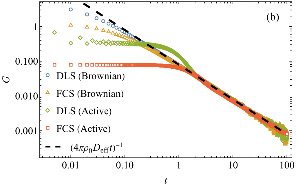
Figure 1 extends FCS and DLS to active baths by comparing simulations of active RTPs and passive BPs in $d=2$ with $V=0$. This minimal setup models the planar measurement of, e.g., active bacteria near surfaces Lemelle et al. 2020 and passive membrane inclusions Lakowicz 2006. The measured signals are $I(t)=\big|\sum_{n}e_{n}(t)e^{i\mathbf{q}\cdot\mathbf{r}_{n}(t)}\big|^{2}$ (DLS) and $I(t)=\sum_{n}e_{n}^{2}(t)$ (FCS), with the detected field $e_{n}(t)\!=\!E_{0}\exp\{-[r_{n}(t)/r_{0}]^{2}\}$. In the active case (see Fig. 1(a)), the RTP dynamics dictate an average persistence length $\ell_{\rm p}=v/\alpha$. On timescales $t\ll\alpha^{-1}$ and length scales $\ell\ll\ell_{\rm p}$, the motion is ballistic, with particles moving in straight lines. For $t\gg\alpha^{-1}$ and $\ell\gg\ell_{\rm p}$, repeated tumbling leads to effective diffusion with $D_{\rm eff}=v^{2}/\alpha d$. In the simulation, the detection radius is $r_{0}=\ell_{\rm p}/\sqrt{2}$ (DLS) and $r_{0}=\ell_{\rm p}$ (FCS), so Fick’s law does not hold on the measurement scale. Nonetheless, the ACF in all settings converges to Eq. (3) in the long-time limit.

Beyond FCS/DLS, Fig. 2 demonstrates Eq. (4) using various local observables. Although Eq. (3) holds in any dimension $d$, Eq. (4) applies only to $d\leq 2$. For $d>2$, the well-known nonuniversal form $\varepsilon^{2}(t)\sim 2\mathcal{D}/t$ is recovered, where the dispersion $\mathcal{D}$ is given by the Green–Kubo relation $\mathcal{D}\!=\!\int_{0}^{\infty}dt\,G(t)$ Tyrrell 1984; Kubo et al. 1991. Nevertheless, dilute $d>1$ systems effectively become non-interacting $d=1$ systems if the measurement projects the dynamics onto a $d=1$ space. This is done by, e.g., probes connected to walls and partitions, where the measurement signal depends solely on motion normal to the wall. Figure 2 thus demonstrates Eq. (4) for two $d=1$ probe models (Fig. 2(a–d)): (I) BPs in a soft box and (II) active RTPs near an asymmetric permeable partition Galajda et al. 2007; Tailleur and Cates 2009; Nikola et al. 2016. To further support the universality, the SM includes two additional models SM: (III) a localized variant of the Ajdari–Prost flashing Brownian ratchet model Ajdari and Prost 1992; Prost et al. 1994; Jülicher et al. 1997 and (IV) random walkers on a lattice, driven by a pointlike pump Sadhu et al. 2011.

Model III is an exact projection of the system in Fig. 2(a) onto the (horizontal) measurement axis foo. In this model, $V(x)$ describes the interaction with soft walls of width $b$ and potential height $V_{0}$ (see Fig. 2(c)). The walls are effectively impenetrable since $V_{0}/T$ is sufficiently large that the typical crossing time far exceeds the acquisition time $\mathcal{T}$ pen; SM. Model III is a simplified model for the projection of the system in Fig. 2(b) onto the measurement axis. In this model, $V(x)$ describes the interaction with a penetrable asymmetric probe of total length $\ell$, potential height $V_{0}$ and side widths $b_{\pm}$ (see Fig. 2(d)) SM.

Two observables are measured for each model. For the equilibrium Model III, these are the net pressure $\mathscr{P}(t)\!=-\!\sum_{n}\!{\rm sgn}(x_{n}(t))f_{n}(t)/2$ exerted on the box walls and the Clausius virial $\mathcal{V}(t)\!=-\!\sum_{n}x_{n}(t)f_{n}(t)/2$, where $f_{n}(t)=-V^{\prime}[x_{n}(t)]$ are the forces exerted on each particle. Both are thermodynamic observables that admit the ideal-gas equations of state $\langle\mathscr{P}\rangle\!=\!\rho_{0}T$ and $\langle\mathcal{V}\rangle\!=-\!\rho_{0}LT/2$. For the far-from-equilibrium Model III, the observables are the net force $F(t)\!=\!\sum_{n}f_{n}(t)$ the probe exerts and the rate $\mathcal{P}(t)$ of total work performed on the particles (consumed power). It is given by $\mathcal{P}(t)\!=\!\sum_{n}p_{n}(t)$, where $p_{n}\!\equiv\!\dot{x}_{n}F_{n}\!-\!\dot{x}_{n}F_{n}|_{f_{n}=0}$ and $F_{n}\!=\!F_{n}(t)$ is the net athermal force exerted on the particle. For Model III, this yields $p_{n}(t)\!=\![\dot{x}_{n}(t)\!+\!vu_{n}(t)]f_{n}(t)$. These observables attain nonvanishing averages only out of equilibrium. In Fig. 2(e), the squared relative uncertainties of all four observables collapse on the universal curve predicted by Eq. (4) in the long-time limit. The above numerical findings motivate a derivation of Eqs. (3-4) from first principles, provided next.

Equations (3-4) follow from the long-time tail of the single-particle conditional probability density (propagator) $P(\mathbf{y},t|\mathbf{y}^{\prime},0)$. Here, the generalized particle coordinate $\mathbf{y}=(\mathbf{r},\mathbf{u})$ includes both its position $\mathbf{r}$ in a $d$-dimensional space of size $L\rightarrow\infty$ and any internal degrees of freedom $\mathbf{u}$, such as momenta of underdamped particles, active particle orientations or shot noise. The propagator long-time tail, derived below, is cn

where $\rho_{\text{s}}(\mathbf{y})$ is the steady-state density, which satisfies $\lim_{r\rightarrow\infty}\int d\mathbf{u}\rho_{\rm s}(\mathbf{r},\mathbf{u})\!=\!\rho_{0}$. The power law in Eq. (7) is a consequence of number conservation Pomeau and Résibois 1975; van Beijeren 1982, which manifests itself for noninteracting particles as probability conservation Tyrrell 1984; Kubo et al. 1991; Mehrer 2007. Indeed, given the initial condition $\rho(\mathbf{y},0)=N\delta(\mathbf{y}-\mathbf{y}^{\prime})$, the average number density $\rho(\mathbf{y},t)$ is given by $\rho(\mathbf{y},t)=NP(\mathbf{y},t|\mathbf{y}^{\prime},0)$. The marginal density $\rho(\mathbf{r},t)=\int d\mathbf{u}\rho(\mathbf{r},\mathbf{u},t)$ is governed by Eq. (1), which lacks an intrinsic relaxation timescale, rendering $\rho(\mathbf{r},t)$ a hydrodynamic mode. Moreover, in the absence of interactions, $\rho(\mathbf{r},t)$ is the only such mode in the system. Equivalently, the position of a particle $\mathbf{r}(t)$ is its only slow degree of freedom.

Equation (7) reveals that the leading order long-time tail is independent of initial conditions ¹¹ 1 $\rho_{\rm{s}}(\mathbf{y})$ is an infinite invariant density, as it is non-normalizable, i.e., $\int d^{d}\mathbf{y}\rho_{\rm{s}}(\mathbf{y})=\infty$. For an overview of infinite invariant densities and infinite ergodic theory, see, e.g. Refs. Aaronson 1997; Aghion et al. 2020. It generalizes previous results for $d=1$ BPs Miyazawa 1999; Aghion et al. 2019; Aghion et al. 2020 and RTPs Granek et al. 2022. Heuristically, $P(\mathbf{y},t|\mathbf{y}^{\prime},0)$ is dominated by particle trajectories that avoid long excursions and remain near $\mathbf{y}$. Such particles forget their initial coordinate $\mathbf{y}^{\prime}$ and relax to a local steady state, i.e $P(\mathbf{y},t|\mathbf{y}^{\prime},0)\sim\rho_{\rm s}(\mathbf{y})$ up to a normalization factor. Since the probability density $P(\mathbf{y},t|\mathbf{y}^{\prime},0)$ expands diffusively at late times, it is supported on a large region of volume $\sim(D_{\rm eff}t)^{d/2}$. This implies a normalization factor $\sim 1/\rho_{0}(D_{\rm eff}t)^{d/2}$.

Equation (7) can be applied to obtain the long-time tails of two-time correlation functions of arbitrary stationary and local observables $A(t)=\sum_{n}a(\mathbf{y}_{n}(t))$ and $B(t)=\sum_{n}b(\mathbf{y}_{n}(t))$, where $\{\mathbf{y}_{n}\!=\!(\mathbf{r}_{n},\mathbf{u}_{n})\}_{n=1}^{N}$ are the generalized coordinates of all particles. Here, local means that $a(\mathbf{y})$ and $b(\mathbf{y})$ decay rapidly for $r=|\mathbf{r}|$ beyond a finite range, with the probe centered at $\mathbf{r}=0$. For $N=\rho_{0}L^{d}$ noninteracting particles, the correlation $\langle A(t)B(0)\rangle_{c}=\langle A(t)B(0)\rangle{-}\langle A\rangle\langle B\rangle$ is given by $N\langle a\left(\mathbf{y}_{1}(t)\right)b\left(\mathbf{y}_{1}(0)\right)\rangle_{c}$. Since $\langle a\rangle=\langle A\rangle/N$, $\langle A(t)B(0)\rangle_{c}$ is expressed explicitly as

with $\mathcal{O}(N^{-1})=\mathcal{O}(L^{-d})$ corrections for finite systems. Inserting Eq. (7) and $\langle A\rangle\!=\!\int d\mathbf{y}\rho_{\rm s}(\mathbf{y})a(\mathbf{y})$ then leads to

Setting $B=A$ then yields the first main result, Eq. (3). Furthermore, for $A(t)=\hat{\rho}(\mathbf{y},t)$ and $B(0)=\hat{\rho}(\mathbf{y}^{\prime},0)$, where $\hat{\rho}(\mathbf{y},t)\equiv\sum_{n}\delta(\mathbf{y}-\mathbf{y}_{n}(t))$ is the empirical density, Eq. (9) provides the density-density correlation function,

where $\langle\hat{\rho}(\mathbf{y})\rangle=\rho_{\rm s}(\mathbf{y})$ is used.

The connection to FCS/DLS can be seen by substituting $A(t)=\int d\mathbf{y}\hat{\rho}(\mathbf{y},t)a(\mathbf{y})$ into Eq. (2), which provides

Equation (11) is the standard equation in FCS theory, with $\mathbf{y}\!=\!\mathbf{r}$, $\rho_{\rm s}(\mathbf{r})\!=\!\rho_{0}$ and $a(\mathbf{r})$ being the probe’s molecule detection efficiency Lakowicz 2006. Each FCS variant uses a model for $a(\mathbf{r})$ in conjunction with the diffusive kernel of noninteracting BPs,

leading to various formulae Blom and Björk 2009, like Eq. (5) for a Gaussian profile. The alternative proposed here is to expand the kernel at $t\rightarrow\infty$, yielding Eq. (3) via Eq. (11), a result which follows more generally from Eq. (10). In DLS, Eq. (11) provides the contribution of particle number fluctuations to $G(t)$ Berne and Pecora 2000. This contribution dominates over $|\mathcal{F}(\mathbf{q},t)|^{2}\!=\!\beta e^{-2D_{\rm eff}q^{2}t}$ for $t\rightarrow\infty$, again recovering Eq. (3).

The second main result, Eq. (4), follows from Eq. (3) and the identity $\varepsilon^{2}(t)\!=\!2t^{-2}\!\int_{0}^{t}\!ds\!\int_{0}^{s}\!ds^{\prime}G(s^{\prime})$ (time-translation invariance). For $d\leq 2$, $\varepsilon^{2}(t)$ decays slower than $\sim t^{-1}$ due to the nonintegrability of $G(t)\sim t^{-d/2}$ and the finite readout $\langle A\rangle\neq 0$. The shift in qualitative behavior for $d\leq 2$ results from recurrence – a non-negligible probability for particles to return to the probe and contribute to $A(t)$ repeatedly Erdős and Dvoretzky 1951; Redner 2001; Majumdar and Schehr 2024 (see Fig. 1(a)). The behavior can be interpreted as anomalous diffusion, where strong correlations cause $\langle\bar{A}^{2}(t)\rangle_{c}$ to grow nonlinearly with time Mandelbrot and Wallis 1968; Dechant et al. 2014; Granek et al. 2022.

In this article, the universal Eqs. (3-4) are derived for local probe measurements in dilute diffusive systems. Together, these equations permit direct local measurement of $D_{\rm eff}$ in microscopic regions — where Fick’s law may fail — and apply broadly across observables and nonequilibrium steady states within the dilute diffusive regime. They can promote existing indirect methods, such as DLS and FCS, which face challenges in short-time measurement of active systems Boon et al. 1974; Wilson et al. 2011; Günther et al. 2018, to direct methods. The only external input required is the macroscopic state variable $\rho_{0}$. Conversely, if $D_{\rm eff}$ is known, the formulae allow direct local measurement of $\rho_{0}$. Put differently, Eq. (3) implies an equation-of-state-like relation,

where $G_{\infty}\equiv\lim_{t\rightarrow\infty}t^{d/2}G(t)$. These predictions may motivate experimental strategies to overcome current barriers to long-term probing Berne and Pecora 2000; Lakowicz 2006; Günther et al. 2018 and the development of novel local probes that measure nonconventional observables. The experimental realization of these possibilities remains open. Several implications of Eq. (4), as well as extensions and relations to prior results, are discussed below.

References

- Pesce et al. (2020) G. Pesce, P. H. Jones, O. M. Maragò, and G. Volpe, Eur. Phys. J. Plus 135, 949 (2020).
- Romero-González et al. (2023) C. Romero-González, B. Morales-Cruzado, D. F. de Lange, R. Romero-Méndez, and F. G. Pérez-Gutiérrez, Opt. Laser Technol. 166, 109691 (2023).
- Crescentini et al. (2014) M. Crescentini, M. Bennati, M. Carminati, and M. Tartagni, IEEE Trans. Biomed. Circuits Syst. 8, 278 (2014).
- Yan and Liu (2025) T. Yan and J. Liu, Angew. Chem. Int. Ed. 64, e202416200 (2025).
- Mehrer (2007) H. Mehrer, Diffusion in Solids (Springer, Berlin Heidelberg, 2007).
- Tyrrell (1984) H. J. V. Tyrrell, Diffusion in Liquids (Elsevier, Amsterdam, 1984).
- Kubo et al. (1991) R. Kubo, M. Toda, and N. Hashitsume, Statistical Physics II, Vol. 31 (Springer, Berlin Heidelberg, 1991).
- Derrida (2007) B. Derrida, J. Stat. Mech. Theory Exp. 2007, P07023 (2007).
- Van Der Ziel and Chenette (1978) A. Van Der Ziel and E. R. Chenette, in Adv. Electron. Electron Phys., Vol. 46 (Academic Press, 1978) pp. 313–383.
- Bonani and Ghione (2001) F. Bonani and G. Ghione, Noise in Semiconductor Devices (Springer Berlin Heidelberg, 2001).
- Dhont (1996) J. Dhont, An Introduction to Dynamics of Colloids (Elsevier, Amsterdam, 1996).
- Webb and Pruess (2003) S. W. Webb and K. Pruess, Transp. Porous Media 51, 327 (2003).
- Tartakovsky and Dentz (2019) D. M. Tartakovsky and M. Dentz, Transp. Porous Media 130, 105 (2019).
- Lorén et al. (2009) N. Lorén, M. Nydén, and A.-M. Hermansson, Adv. Colloid Interface Sci. 150, 5 (2009).
- Jee et al. (2018) A.-Y. Jee, Y.-K. Cho, S. Granick, and T. Tlusty, Proc. Natl. Acad. Sci. U.S.A 115, E10812 (2018).
- Feng and Gilson (2020) M. Feng and M. K. Gilson, Annu. Rev. Biophys. 49, 87 (2020).
- Ghosh et al. (2021) S. Ghosh, A. Somasundar, and A. Sen, Annu. Rev. Condens. Matter Phys. 12, 177 (2021).
- Granek et al. (2024) O. Granek, Y. Kafri, M. Kardar, S. Ro, J. Tailleur, and A. Solon, Rev. Mod. Phys. 96, 031003 (2024).
- Gordon (1945) A. R. Gordon, Ann. N. Y. Acad. Sci. 46, 285 (1945).
- Tanford (1961) C. Tanford, Physical Chemistry of Macromolecules (John Wiley & Sons, Hoboken, NJ, 1961).
- Rutherford and Do (1997) S. W. Rutherford and D. D. Do, Adsorption 3, 283 (1997).
- Lee et al. (2017) J. K. Lee, S. X. Yao, G. Li, M. B. G. Jun, and P. C. Lee, Polym. Rev. 57, 695 (2017).
- Nguyen et al. (2022) H.-T. Nguyen, A. Bouchaudy, and J.-B. Salmon, Phys. Fluids 34, 52008 (2022).
- Hamada and de Anna (2023) M. Hamada and P. de Anna, Transp. Porous Media 146, 463 (2023).
- Manzo and Garcia-Parajo (2015) C. Manzo and M. F. Garcia-Parajo, Rep. Prog. Phys. 78, 124601 (2015).
- Shen et al. (2017) H. Shen, L. J. Tauzin, R. Baiyasi, W. Wang, N. Moringo, B. Shuang, and C. F. Landes, Chem. Rev. 117, 7331 (2017).
- Kumar et al. (2023) A. Kumar, Y. Scher, S. Reuveni, and M. S. Santhanam, Phys. Rev. Res. 5, L032043 (2023).
- Price (2009) W. S. Price, NMR Studies of Translational Motion (Cambridge University Press, Cambridge, 2009).
- Kärger and Valiullin (2013) J. Kärger and R. Valiullin, Chem. Soc. Rev. 42, 4172 (2013).
- Berne and Pecora (2000) B. J. Berne and R. Pecora, Dynamic light scattering (Dover Publications, Mineola, NY, 2000).
- Stetefeld et al. (2016) J. Stetefeld, S. A. McKenna, and T. R. Patel, Biophys. Rev 8, 409 (2016).
- Krichevsky and Bonnet (2002) O. Krichevsky and G. Bonnet, Rep. Prog. Phys 65, 251 (2002).
- Lakowicz (2006) J. R. Lakowicz, Principles of Fluorescence Spectroscopy (Springer, Boston, MA, 2006).
- Günther et al. (2018) J.-P. Günther, M. Börsch, and P. Fischer, Acc. Chem. Res. 51, 1911 (2018).
- Yu et al. (2021) L. Yu, Y. Lei, Y. Ma, M. Liu, J. Zheng, D. Dan, and P. Gao, Front. Phys. 9, 644450 (2021).
- Lorén et al. (2015) N. Lorén, J. Hagman, J. K. Jonasson, H. Deschout, D. Bernin, F. Cella-Zanacchi, A. Diaspro, J. G. McNally, M. Ameloot, N. Smisdom, M. Nydén, A.-M. Hermansson, M. Rudemo, and K. Braeckmans, Q. Rev. Biophys. 48, 323 (2015).
- Pincet et al. (2016) F. Pincet, V. Adrien, R. Yang, J. Delacotte, J. E. Rothman, W. Urbach, and D. Tareste, PLoS One 11, e0158457 (2016).
- Boon et al. (1974) J. P. Boon, R. Nossal, and S.-H. Chen, Biophys. J. 14, 847 (1974).
- Wilson et al. (2011) L. G. Wilson, V. A. Martinez, J. Schwarz-Linek, J. Tailleur, G. Bryant, P. N. Pusey, and W. C. K. Poon, Phys. Rev. Lett. 106, 018101 (2011).
- Kandula et al. (2019) H. N. Kandula, A. Y. Jee, and S. Granick, J. Phys. Chem. A 123, 10184 (2019).
- Jee et al. (2019) A.-Y. Jee, K. Chen, T. Tlusty, J. Zhao, and S. Granick, J. Am. Chem. Soc 141, 20062 (2019).
- Jee et al. (2020) A.-Y. Jee, T. Tlusty, and S. Granick, Proc. Natl. Acad. Sci. U.S.A 117, 29435 (2020).
- Erdős and Dvoretzky (1951) P. Erdős and A. Dvoretzky, Berkeley Symp. Math. Statist. Probab. 2, 353 (1951).
- Redner (2001) S. Redner, A guide to first-passage processes (Cambridge University Press, Cambridge, 2001).
- Majumdar and Schehr (2024) S. N. Majumdar and G. Schehr, (2024), arXiv:2405.20955 [cond-mat.stat-mech] .
- Höfling et al. (2011) F. Höfling, K.-U. Bamberg, and T. Franosch, Soft Matter 7, 1358 (2011).
- Höfling and Franosch (2013) F. Höfling and T. Franosch, Rep. Prog. Phys. 76, 046602 (2013).
- Banks et al. (2016) D. S. Banks, C. Tressler, R. D. Peters, F. Höfling, and C. Fradin, Soft Matter 12, 4190 (2016).
- Blom and Björk (2009) H. Blom and G. Björk, Appl. Opt. 48, 6050 (2009).
- Cates (2012) M. E. Cates, Rep. Prog. Phys. 75, 042601 (2012).
- Schnitzer (1993) M. J. Schnitzer, Phys. Rev. E 48, 2553 (1993).
- (52) A logarithmic moving average of windows was further applied to BP DLS data.
- Lemelle et al. (2020) L. Lemelle, T. Cajgfinger, C. C. Nguyen, A. Dominjon, C. Place, E. Chatre, R. Barbier, J.-F. Palierne, and C. Vaillant, Biophys. J. 118, 2400 (2020).
- Galajda et al. (2007) P. Galajda, J. Keymer, P. Chaikin, and R. Austin, J. Bacteriol. 189, 8704 (2007).
- Tailleur and Cates (2009) J. Tailleur and M. E. Cates, EPL 86, 60002 (2009).
- Nikola et al. (2016) N. Nikola, A. P. Solon, Y. Kafri, M. Kardar, J. Tailleur, and R. Voituriez, Phys. Rev. Lett. 117, 098001 (2016).
- (57) See Supplemental Material at [URL], which includes Refs. Kitahara et al. 1979; Szavits-Nossan et al. 2017; Shiraishi 2023, for further simulation details and additional probe examples.
- Ajdari and Prost (1992) A. Ajdari and J. Prost, C. R. Acad. Sci. Paris II 315, 1635 (1992).
- Prost et al. (1994) J. Prost, J.-F. Chauwin, L. Peliti, and A. Ajdari, Phys. Rev. Lett. 72, 2652 (1994).
- Jülicher et al. (1997) F. Jülicher, A. Ajdari, and J. Prost, Rev. Mod. Phys. 69, 1269 (1997).
- Sadhu et al. (2011) T. Sadhu, S. N. Majumdar, and D. Mukamel, Phys. Rev. E 84, 051136 (2011).
- (62) This follows directly from the separability of the original dynamics in Cartesian coordinates.
- (63) The wall penetrability does not affect the equations of state and the validity of the results.
- (64) The expansion is taken with and fixed and , i.e. for . For finite-yet-large , the long-time tails are valid for , after which the decay becomes exponential. The slow decay then materializes as a dependence of on .
- Pomeau and Résibois (1975) Y. Pomeau and P. Résibois, Phys. Rep. 19, 63 (1975).
- van Beijeren (1982) H. van Beijeren, Rev. Mod. Phys. 54, 195 (1982).
- (67) is an infinite invariant density, as it is non-normalizable, i.e., . For an overview of infinite invariant densities and infinite ergodic theory, see, e.g. Refs. Aaronson 1997; Aghion et al. 2020.
- Aaronson (1997) J. Aaronson, An Introduction to Infinite Ergodic Theory (American Mathematical Society, Providence, RI, 1997).
- Miyazawa (1999) T. Miyazawa, J. Math. Phys. 40, 838 (1999).
- Aghion et al. (2019) E. Aghion, D. A. Kessler, and E. Barkai, Phys. Rev. Lett. 122, 010601 (2019).
- Aghion et al. (2020) E. Aghion, D. A. Kessler, and E. Barkai, Chaos Solitons Fractals 138, 109890 (2020).
- Granek et al. (2022) O. Granek, Y. Kafri, and J. Tailleur, Phys. Rev. Lett. 129, 038001 (2022).
- Mandelbrot and Wallis (1968) B. B. Mandelbrot and J. R. Wallis, Water Resour. Res. 4, 909 (1968).
- Dechant et al. (2014) A. Dechant, E. Lutz, D. A. Kessler, and E. Barkai, Phys. Rev. X 4, 011022 (2014).
- (75) Any bound states maintain a finite gap as .
- Griffiths and Schroeter (2018) D. J. Griffiths and D. F. Schroeter, Introd. to Quantum Mech. (Cambridge University Press, Cambridge, 2018).
- Van Kampen (1985) N. G. Van Kampen, Phys. Rep. 124, 69 (1985).
- Gardiner (1985) C. W. Gardiner, Handbook of Stochastic Methods (Springer, Berlin Heidelberg, 1985).
- (79) Eq. (17) is equivalent to , where is a projection operator.
- Seifert (2019) U. Seifert, Annu. Rev. Condens. Matter Phys. 10, 171 (2019).
- Di Terlizzi and Baiesi (2019) I. Di Terlizzi and M. Baiesi, J. Phys. A 52, 02LT03 (2019).
- Busiello and Pigolotti (2019) D. M. Busiello and S. Pigolotti, Phys. Rev. E 100, 060102(R) (2019).
- Van Vu et al. (2020) T. Van Vu, V. T. Vo, and Y. Hasegawa, Phys. Rev. E 101, 042138 (2020).
- Shiraishi (2021) N. Shiraishi, J. Stat. Phys. 185, 19 (2021).
- Busiello and Fiore (2022) D. M. Busiello and C. E. Fiore, J. Phys. A 55, 485004 (2022).
- Dieball and Godec (2023) C. Dieball and A. Godec, Physical Review Letters 130, 087101 (2023).
- Timpanaro et al. (2023) A. M. Timpanaro, G. Guarnieri, and G. T. Landi, Phys. Rev. B 107, 115432 (2023).
- Agmon et al. (1988) N. Agmon, E. Pines, and D. Huppert, J. Chem. Phys. 88, 5631 (1988).
- Agmon (2011) N. Agmon, Phys. Chem. Chem. Phys. 13, 16548 (2011).
- Simkovitch et al. (2016) R. Simkovitch, D. Pines, N. Agmon, E. Pines, and D. Huppert, . Phys. Chem. B. 120, 12615 (2016).
- Sivan and Farago (2018) M. Sivan and O. Farago, Phys. Rev. E 98, 052117 (2018).
- Defaveri et al. (2023) L. Defaveri, E. Barkai, and D. A. Kessler, Phys. Rev. E 107, 024122 (2023).
- Darling and Kac (1957) D. A. Darling and M. Kac, Trans. Am. Math. Soc. 84, 444 (1957).
- Bouchaud et al. (1990) J. P. Bouchaud, A. Comtet, A. Georges, and P. Le Doussal, Ann. Phys. (N. Y). 201, 285 (1990).
- Bouchaud and Georges (1990) J.-P. Bouchaud and A. Georges, Phys. Rep. 195, 127 (1990).
- Seyforth et al. (2022) H. Seyforth, M. Gomez, W. B. Rogers, J. L. Ross, and W. W. Ahmed, Phys. Rev. Res. 4, 023043 (2022).
- Venturelli et al. (2024) D. Venturelli, S. A. M. Loos, B. Walter, É. Roldán, and A. Gambassi, EPL 146, 27001 (2024).
- Van Kampen and Oppenheim (1986) N. G. Van Kampen and I. Oppenheim, Phys. A Stat. Mech. its Appl. 138, 231 (1986).
- D’Alessio et al. (2016) L. D’Alessio, Y. Kafri, and A. Polkovnikov, J. Stat. Mech. Theory Exp. 2016, 023105 (2016).
- Maes (2020) C. Maes, Phys. Rev. Lett. 125, 208001 (2020).
- Solon and Horowitz (2022) A. Solon and J. M. Horowitz, J. Phys. A 55, 184002 (2022).
- Lifson and Jackson (1962) S. Lifson and J. L. Jackson, J. Chem. Phys. 36, 2410 (1962).
- Derrida (1983) B. Derrida, J. Stat. Phys. 31, 433 (1983).
- Vergassola and Avellaneda (1997) M. Vergassola and M. Avellaneda, Phys. D Nonlinear Phenom. 106, 148 (1997).
- Dean et al. (2007) D. S. Dean, I. T. Drummond, and R. R. Horgan, J. Stat. Mech. Theory Exp. 2007, P07013 (2007).
- Luck and Mehta (2001) J. M. Luck and A. Mehta, Europhysics Letters (EPL) 54, 573 (2001), arXiv:0008400 [cond-mat] .
- Dhar (2008) A. Dhar, Adv. Phys. 57, 457 (2008).
- Ernst (2005) M. H. Ernst, Phys. Rev. E 71, 030101 (2005).
- Ripoll and Ernst (2005) M. Ripoll and M. H. Ernst, Phys. Rev. E 72, 011101 (2005).
- Kitahara et al. (1979) K. Kitahara, W. Horsthemke, and R. Lefever, Phys. Lett. A 70, 377 (1979).
- Szavits-Nossan et al. (2017) J. Szavits-Nossan, M. R. Evans, and S. N. Majumdar, J. Phys. A 50, 024005 (2017).
- Shiraishi (2023) N. Shiraishi, An Introduction to Stochastic Thermodynamics: From Basic to Advanced (Springer, Singapore, 2023).