B-stability of numerical integrators on Riemannian manifoldsThanks: * Corresponding authorThanks: This work was supported by the European Union’s Horizon 2020 research and innovation programme under the Marie Skłodowska-Curie grant agreement No. 860124. This publication reflects only the author’s view and the Research Executive Agency is not responsible for any use that may be made of the information it contains.
Abstract.
We propose a generalization of nonlinear stability of numerical one-step integrators to Riemannian manifolds in the spirit of Butcher’s notion of B-stability. Taking inspiration from Simpson-Porco and Bullo, we introduce non-expansive systems on such manifolds and define B-stability of integrators. In this first exposition, we provide concrete results for a geodesic version of the Implicit Euler (GIE) scheme. We prove that the GIE method is B-stable on Riemannian manifolds with non-positive sectional curvature. We show through numerical examples that the GIE method is expansive when applied to a certain non-expansive vector field on the 2-sphere, and that the GIE method does not necessarily possess a unique solution for large enough step sizes. Finally, we derive a new improved global error estimate for general Lie group integrators.
Key words and phrases:
B-stability, Riemannian manifolds, contractivity, numerical integrators on manifolds2020 Mathematics Subject Classification
Primary: 65L20. Secondary: 34C40, 53-08, 58D17, 65L051. Introduction
Stability is a fundamental property of numerical methods for stiff nonlinear ordinary differential equations. It is important for controlling the growth of error in the numerical approximation and is used in combination with local error estimates to obtain bounds for the global error. Stability bounds can also in some situations be used to ensure the existence and uniqueness of a solution to the algebraic equations arising from implicit integrators. In the literature, one can find a large variety of stability definitions for numerical integrators with various different aims. Some of them apply to linear test equations, others are of a more general nature and apply to nonlinear problems with certain prescribed properties. Most of the stability definitions found in the literature are developed for problems modeled on linear spaces. In particular, there is a well-established non-linear stability theory, where an inner product norm is used to measure the distance between two solutions and the corresponding numerical approximations. Pioneering contributions to this theory were made by Dahlquist and Butcher in the mid-1970s [17, 6], in the wake of the legendary numerical analysis conference in Dundee, 1975. The notions of G-stability for multi-step methods [17] and B-stability of Runge–Kutta methods [6] were developed. The overall idea of B-stability is that whenever the norm of the difference between two solutions of the ODE is monotonically non-increasing, the numerical method should exhibit a similar behavior, that is, the difference in norm between the two corresponding numerical solutions should not increase over a time step. Much is known about B-stable Runge–Kutta methods, and there is even an algebraic condition on the coefficients of a method that ensures its B-stability. A key ingredient is the one-sided Lipschitz condition, also called a monotonicity condition, on the ODE vector field. We refer the reader to the excellent monographs [24, 20] for a detailed treatment of the various definitions of stability and B-stability in particular.
We remark that whether a particular ODE system is non-expansive depends on the choice of inner product norm, but the notion of a B-stable Runge–Kutta method does not, see [24]*p. 182. In this paper, we shall be concerned with unconditional stability, meaning that step sizes are allowed. This excludes all explicit integrators, and it makes it necessary to assume that both the flow of the ODE vector field and the numerical method map are well defined for all positive . Dahlquist and Jeltsch [18] introduced generalized disks of contractivity in order to consider also the case in which limitations on the ODE vector field and the step size are imposed.
We shall here consider systems of ODEs whose solutions evolve on a smooth manifold. We are primarily interested in numerical integrators which are intrinsic, that are not developed for a particular choice of local coordinates, or based on a specific embedding of the manifold into an ambient space. There are several such numerical methods available in the literature.
Crouch and Grossman [15] proposed to build integrators by composing flows of so-called frozen vector fields, and these methods were later extended to a more general format in [10] called Commutator-free Lie group methods. Munthe–Kaas introduced numerical integrators for homogeneous spaces [41] by equipping the manifold with a left transitive Lie group action which was used together with the exponential map to transform the ODE vector field locally to a vector field on the underlying Lie algebra. Its flow is approximated by any classical Runge–Kutta method, and the result is mapped back to the manifold by composing the group action with the exponential map.
In computational mechanics there were early contributions to numerical integration on particular manifolds, such as the rotation group and the special Euclidean group . A landmark paper in the design of conservative methods for Hamiltonian systems on Lie groups is the one by Lewis and Simo [37]. For rod dynamics, an important paper was that of Simo and Vu-Quoc [46] who developed a geometrically exact formulation for rods undergoing large motions, and for the time stepping they devised a version of the Newmark methods applicable to Lie groups. These methods can be generalized to the so-called -methods [27] in a Lie group setting, see [2, 3]. Parametrization of the manifold in question, such as the rotation group, plays a significant role in computational mechanics, for efficiency, accuracy, and storage requirements. When using (minimal) local coordinates for global simulation, one inevitably runs into problems with singularities, these issues have been studied and amended by several authors, e.g. [48, 28]. Hamiltonian systems are often formulated on cotangent bundles, in which case symplectic integrators can be derived through the discretization of a variational problem, this approach is sometimes named discrete mechanics. The pioneering work by Marsden and West [38] developed this theory for Euclidean spaces, and it has later been generalized to Lie groups in a number of papers [34, 5, 11, 21, 25, 26, 36].
Finally, on a Riemannian manifold, it is natural to base the numerical schemes primarily on the Riemannian exponential map. Leimkuhler and Patrick [35] derived a symplectic integrator for Riemannian manifolds, and in [12] the authors suggest using Riemannian normal coordinates to define a retraction map.
For an in-depth account of Lie group methods, we refer to [30, 14, 11, 42, 7] and references therein.
In this paper we shall make the first attempt to generalize B-stability to Riemannian manifolds, replacing the inner product norm with the Riemannian distance function. We take inspiration from the work of Simpson-Porco and Bullo [47] who considered contraction properties of a continuous system. In Section 2 we define what we mean by a non-expansive system on a Riemannian manifold, and we state the definition of B-stability of a general numerical method in this setting. Then, in Section 3 we first present two examples of numerical methods: the geodesic versions of the implicit Euler method (GIE) and the implicit midpoint rule (GIMP). Then we prove a B-stability result for the GIE method in the case that the manifold has non-positive sectional curvature. We also provide numerical experiments for a particular vector field on the two-sphere, , showing that neither the GIE nor the GIMP method is B-stable on this manifold which has positive sectional curvature. We briefly discuss also for this example a non-uniqueness issue with the GIE method which is different from what is known from the Euclidean setting. Finally, in Section 4 we present a bound for the global error of numerical methods, based on the monotonicity condition.
2. Non-expansive systems
We begin by briefly introducing some notation and terminology, mostly adhering to the monograph by Lee [33]. A Riemannian manifold is a pair , where is a smooth manifold and is a smoothly varying inner product defined on each tangent space . We will use interchangeably the notations and . Associated to is the Levi-Civita connection, the unique affine connection , which for any three vector fields on satisfies and . The connection also defines the covariant derivative of vector fields along curves, we use the notation to denote the covariant derivative of along , see [33]*Theorem 4.21. A curve is geodesic if it satisfies the equation along . A geodesic that connects two points and is called a geodesic segment. If this second order differential equation, together with initial data yields a solution , , thus . A similar notation is used for the -flow, , of a vector field on , it is the diffeomorphism on , where , and its domain of definition may be -dependent. A numerical method on M is a map that approximates the flow map . A set is geodesically convex if, for each , there is a unique minimizing geodesic segment from to contained entirely in . A vector field is forward complete on if for every , is defined for all . If for every it holds that , we say that is forward -invariant. Similarly, for a mapping the set is -invariant if for any . We denote the length of a curve as , where is the -norm. The metric induces a distance function between pairs of points , , where is any continuous curve connecting and . The following definition replaces the one-sided Lipschitz condition on a Riemannian manifold.
Definition 2.1.
Let be a Riemannian manifold and let . We say that the vector field satisfies a monotonicity condition on the set with constant if for every and , it holds that
| (2.1) |
Consider for every , the linear operator on . The constant can be chosen as
| (2.2) |
where is the logarithmic -norm of . For a linear operator , its logarithmic -norm is defined as [20]
In local coordinates on , we write the vector field as and the metric tensor is represented by the matrix with elements . The operator has the matrix representation where and where are the Christoffel symbols of the connection. We can now formulate the logarithmic -norm of pointwise as
i.e., the largest eigenvalue of the matrix in square brackets, see also [19].
Theorem 2.2.
Let be a Riemannian manifold, a geodesically convex set, and let be a vector field on satisfying the monotonicity condition (2.1) on with a constant . Suppose that for any , there is a such that and exist and are contained in for every . Then, it holds that
| (2.3) |
Remark 2.3.
The condition that the set is geodesically convex can be weakened by introducing the notion of a -reachable set as in [47].
Proof.
The construction for the proof is illustrated in Figure 1. Since is geodesically convex, there is a unique minimizing geodesic connecting , with and . We will be using the notation , as in [33]*Chapter 6, and is contained in . For a fixed , consider the length of the curve , , that is
| (2.4) |
and we have . Let
| (2.5) |
We will use that
following from the symmetry lemma [33]*Lemma 6.2. Differentiating with respect to , using the chain rule and the properties of the Levi-Civita connection, we have
where the last inequality follows from the assumption that satisfies the monotonicity condition (2.1). By Gronwall’s lemma, we obtain the inequality
and conclude that
∎
Remark 2.4.
Choosing leads to a bound similar to the one in Theorem 1.2 by Kunzinger et al. in [32].
The next definition is inspired by the definition of contracting systems by Simpson-Porco and Bullo in [47].
Definition 2.5 (Non-expansive system).
Let be a Riemannian manifold. Let be an open, geodesically convex set and . If
- (i)
is forward complete on ,
- (ii)
is forward -invariant,
- (iii)
satisfies the monotonicity condition (2.1) on with ,
the quadruple is called a non-expansive system.
We are now ready to give the definition of a B-stable numerical method on Riemannian manifolds.
Definition 2.6 (B-stability).
Let be a Riemannian manifold and let be a numerical method on . Suppose that for any non-expansive system on , it holds that
- (i)
is forward complete on , i.e., is well defined for all , and
- (ii)
is forward -invariant for all .
If
then is called B-stable.
3. Numerical integrators on manifolds and B-stability
Geodesic Explicit Euler (GEE) method
The simplest numerical method defined on a Riemannian manifold is the Geodesic Explicit Euler method
| (3.1) |
that can not be unconditionally stable, but will be used for comparison in the numerical experiments in Example 3.2.
Geodesic Implicit Euler (GIE) method
We consider the following definition of the Implicit Euler method in a Riemannian manifold
| (3.2) |
This reduces to the classical implicit Euler method when the manifold is the Euclidean space.
Geodesic Implicit Midpoint (GIMP) method
Similarly, we consider the implicit midpoint rule on a Riemannian manifold:
| (3.3) | ||||
This method can be found in Zanna et al. [50] for the case of Lie group integrators. It is a symmetric method, but it is not generally symplectic. In [39] a symplectic method was found for products of 2-spheres, , that happens to be a time reparametrization of (3.3). It is called the spherical midpoint method (SPHMP). Applied to a single copy of it reads in Cartesian coordinates
| (3.4) |
3.1. The case with non-positive sectional curvature
In the next theorem, we prove the B-stability of the GIE method on Hadamard manifolds, i.e., manifolds with non-positive sectional curvature.
Theorem 3.1 (B-stability of the GIE method).
Let be a Riemannian manifold with non-positive sectional curvature. Then, the GIE method (3.2) is B-stable.
Proof.
Let be a non-expansive system of ODEs, and consider with step size . Let be a curve in such that and , and set . By assumption is well defined and contained in . Consider the one-parameter family of curves
We have and . Now, using as earlier the notation , we have
Let . We differentiate with respect to and apply the Jacobi equation together with the definition of sectional curvature and obtain
| (3.5) | ||||
Here is the Riemannian curvature tensor and is the sectional curvature. Since by assumption it follows that for . By the symmetry lemma [33]*Lemma 6.2, we get
Then
since satisfies the monotonicity condition with . So, we have
which allows us to conclude that . Thus
| (3.6) |
For any given , we have . By (3.6) and the definition of distance we obtain
Since is arbitrary, the condition for B-stability is satisfied. ∎
Example 3.2.
[] The space of symmetric positive definite matrices is a well-known example of a manifold with negative sectional curvature. Its tangent space at a point , denoted by , can be identified as the set of symmetric matrices. is equipped pointwise with the metric
| (3.7) |
The manifold can be used as a model space for simple beam models, such as the Elastica [51], or in diffusion tensor magnetic resonance imaging (DT-MRI) [13, 44, 8, 22], via 3D tensors, i.e., SPD matrices. Another interesting application is the segmentation and recognition of images and videos represented by SPD matrices, [1, 29, 49]. Such applications usually involve averaging SPD matrices, for example, to collect noisy measurements of the object under consideration. In , a suitable mean was proposed by Karcher [31]. Given matrices , we search for a matrix , the Karcher mean, such that
| (3.8) |
i.e., is such that . Here, is the Riemannian distance between and given as [23]
| (3.9) |
with being the eigenvalue of , and grad is the Riemannian gradient found e.g. in [23]*Lemma 2
| (3.10) |
For , the exponential map is explicitly known in terms of the matrix exponential and matrix square roots as
for and
The objective function is defined as the geometric mean of symmetric positive definite matrices in [40] and [4], and is known to have a unique minimizer as in (3.8), [31].
There is no known closed-form solution for (3.8) and usually, iterative methods are used to compute the Karcher mean.
In Figure 2, the Riemannian distance of two solutions after one step is plotted for increasing values of the step size with the same pair of initial values. One can observe the non-expansive behavior of the GIE and the GIMP method and the expansive behavior of the Geodesic Explicit Euler (GEE) method. The GEE solution is discontinued at for presentation purposes. The exact solution is calculated with strict tolerance by odeint of scipy.integrate in Python.
3.2. The case with positive sectional curvature: The 2-sphere
In this section, we consider systems on the 2-sphere with the standard metric. We show through an example that the GIE and GIMP methods fail to be B-stable.
3.2.1. Killing vector fields
A Killing vector field is a vector field such that the Lie derivative . This implies that
so that the monotonicity condition (2.1) holds with for any such vector field. In this sense one could say that the Killing vector fields represent a borderline case for non-expansive systems.
3.2.2. A Killing vector field on
Consider the vector field , which describes rotations on the 2-sphere around the -axis. Using Cartesian coordinates, the GIE method (3.2) on the 2-sphere takes the form
| (3.11) |
We apply (3.11) to two initial points lying on the open northern hemisphere and measure the distance between the points for increasing values of the time step. The distance between two points is calculated as
| (3.12) |
Figure 3 (left) shows one step performed with the GIE method starting from two initial points with increasing step size . In Figure 3 (right), the distance between the trajectories is shown as a function of . As can be seen from the distance curve, the GIE method shows an expansive behavior, and it is in fact small values of the step size that cause problems. In Figure 4, the SPHMP and the GIMP methods are tested on the same vector field. Both methods are a reparametrization of the exact solution for this problem.
A non-uniqueness issue
It is well-known from the theory of implicit Runge–Kutta methods that the conditions for the uniqueness of the solution to the implicit equations that must be solved in each time step involve the one-sided Lipschitz condition. In the monograph by Hairer and Wanner [24] a precise result is given, and we include it here for completeness.
Theorem 3.3 (Theorem 14.4 in [24]).
Consider a differential equation satisfying a one-sided Lipschitz condition with constant . If the Runge–Kutta matrix is invertible and , then the system of equations to be solved in each time step possesses at most one solution.
We note that is a function that depends only on the Runge–Kutta coefficients, and it is known that for the implicit Euler method. Thus, for there is a unique solution for every . But the Killing vector field example on shows that this result is not generally true in Riemannian manifolds. In fact, for this example, we see from (3.11) that the last component is decoupled from the other two. Writing for simplicity and we need to solve the scalar equation
| (3.13) |
with respect to . One has for all , and for for any such that . In fact, for , has precisely one zero, and for , , has zeros in . All the zeros are simple and therefore there is a sign change in at each of them. It follows that such that if and , then (3.13) has at least solutions. One easily verifies that for each of these values of the last component, there is a unique solution for the first two components. We illustrate the structure of the solution in Figure 5.
3.2.3. Relation to other Lie group integrators
For some homogeneous manifolds , with a closed Lie subgroup of the Lie group , the Geodesic Implicit Euler method (3.2) is equivalent to the implicit Lie-Euler method for a specific choice of isotropy, [41, 11], i.e., of the map which is used to define the Lie group method:
| (3.14) |
with the Lie algebra of and the Lie group exponential. See [30] for an introduction to Lie group methods. The following example on illustrates the impact of the choice of isotropy on the approximation of the solution obtained via (3.14).
Example 3.4.
Consider a vector field on the 2-sphere . In Cartesian coordinates, embedding in , the ODE can be written as
| (3.15) |
where denotes the vector cross product. By the identification of with the Lie algebra , we have that . The action of the Lie group exponential on a vector takes the simple form:
We remark that for a given vector field , the choice of is not unique. In fact, we can replace with its projection orthogonal to without changing , and similarly replacing by , with , does not alter :
On the other hand, the numerical approximation obtained by the method (3.14),
does depend on the choice of , see also Figure 6. Similarly, we cannot expect that in general different Lie group integrators have the same stability behavior when applied to the same vector field .
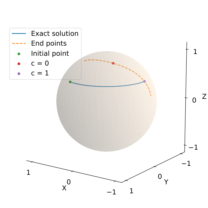
In Figure 6 we illustrate the isotropy issue by applying the Implicit Lie–Euler method
to the problem
| (3.16) |
for and step size . This means that corresponds to the GIE method, whereas for the exact solution is reproduced. We observe that the difference in solutions may expand, contract or stay constant, depending on the choice of isotropy parameter .
4. A bound for the global error
For the next result, we first consider an initial value problem on the finite-dimensional Riemannian manifold
| (4.1) |
where is a smooth vector field, is the initial value. The following theorem is a generalization of Theorem 2 from [9], where we use the constant from the monotonicity condition rather than the operator norm of .
Theorem 4.1.
Let be a Riemannian manifold and fix . Let be a geodesically convex set and a vector field on satisfying the monotonicity condition (2.1) on with constant . Let be defined and contained in for . Let be a numerical method , well defined and contained in for any such that , whose local error can be bounded for some and as
| (4.2) |
Then, for all , the global error is bounded as
| (4.3) |
Proof.
Let us denote the global error as . For
| (4.4) | ||||
| (4.5) | ||||
| (4.6) |
(4.4) is the triangle inequality, where the first term is the error at propagated over one step and the second term is the local error. (4.5) is obtained via a Grönwall-type inequality of [32] for the first term. Using the local error estimate (4.2) for the second term we obtain the recursion in (4.6). Considering , and summing over , we obtain
| (4.7) |
For , and (4.7) becomes equivalent to the first estimate in (4.3). For , and (4.7) becomes equivalent to the third estimate in (4.3). ∎
Remark 4.2.
In cases where the monotonicity constant , in the sense that one can assume as , see e.g. [24]*Ch IV.15, one gains an order of convergence such that the global error essentially equals the local error.
5. Conclusions and further work
The notion of B-stability proposed in [6] for Euclidean spaces has been generalized to Riemannian manifolds. Building on the work by Simpson-Porco and Bullo [47] on contraction systems in Riemannian manifolds, we expressed the B-stability condition in terms of the Riemannian distance function. For this first study, only geodesic versions of the implicit Euler method and the implicit midpoint rule were considered. We proved that in the Riemannian setting, the geodesic implicit Euler method is B-stable for manifolds of non-positive sectional curvature, but not necessarily in positively curved spaces. Through numerical experiments on the 2-sphere, one finds strong evidence that the GIE method is indeed not B-stable in general. Another observation was that, contrary to what has been proved in Euclidean spaces, the nonlinear equations associated with the GIE method do not have a unique solution for non-expansive systems. Finally, we showed that the monotonicity constant can be used to obtain improved global error estimates compared to [16, 9].
Many open questions remain for the B-stability properties of numerical methods applied to problems on Riemannian manifolds. There exist many classes of numerical integrators that could be analyzed in this setting. In mechanical engineering, most of the problems of interest are set in manifolds of positive sectional curvature, such as , , and direct or semidirect products of these. It may also be of interest to consider explicit integrators, in which case B-stability must be replaced by some conditional form of stability, such as the circle contractivity proposed in [18].
References
- [1] O. Arandjelovic, G. Shakhnarovich, J. Fisher, R. Cipolla and T. Darrell, Face recognition with image sets using manifold density divergence, Computer Society Conference on Computer Vision and Pattern Recognition (CVPR’05), 2005, 581-588.
- [2] M. Arnold and O. Brüls, Convergence of the generalized- scheme for constrained mechanical systems, Multibody System Dynamics 18 (2007), no. 2, 185–202.
- [3] M. Arnold, O. Brüls and A. Cardona, Error analysis of generalized- Lie group time integration methods for constrained mechanical systems, Numerische Mathematik 129 (2015), no. 1, 149-179.
- [4] R. Bhatia and J. Holbrook, Riemannian geometry and matrix geometric means, Linear algebra and its applications, 413 (2006), no. 2-3, 594-618.
- [5] G. Bogfjellmo and H. Marthinsen, High-order symplectic partitioned Lie group methods, Foundations of Computational Mathematics 16 (2016), no. 2, 493-530.
- [6] J.C. Butcher, A stability property of implicit Runge-Kutta methods, BIT 15 (1975), 358-361.
- [7] E. Celledoni, E. Çokaj, A. Leone, D. Murari and B. Owren, Lie group integrators for mechanical systems, International Journal of Computer Mathematics 99 (2021), no. 8, 1-31.
- [8] E. Celledoni, S. Eidnes and B. Owren and T. Ringholm, Dissipative numerical schemes on Riemannian manifolds with applications to gradient flows, SIAM Journal on Scientific Computing 40 (2018), no. 6, 3789-3806.
- [9] E. Celledoni, S. Eidnes, B. Owren and T. Ringholm, Energy-preserving methods on Riemannian manifolds, Mathematics of Computation 89 (2020), no. 322, 699-716.
- [10] E. Celledoni, A. Marthinsen and B. Owren, Commutator-free Lie group methods, Future Generation Computer Systems 19 (2003), 341-352.
- [11] E. Celledoni, H. Marthinsen and B. Owren, An introduction to Lie group integrators - basics, new developments and applications, Journal of Computational Physics 257 (2014), no. part B, 1040-1061.
- [12] E. Celledoni and B. Owren, A class of intrinsic schemes for orthogonal integration, SIAM Journal on Numerical Analysis 40, (2002), no. 6, 2069-2084.
- [13] G. Cheng, H. Salehian and B. C. Vemuri, Efficient recursive algorithms for computing the mean diffusion tensor and applications to DTI segmentation, Computer Vision-ECCV 2012: 12th European Conference on Computer Vision, Florence, Italy, October 7-13, 2012, Proceedings Part VII 12, (2012), 390-401.
- [14] S. H. Christiansen, H. Z. Munthe-Kaas and B. Owren, Topics in structure-preserving discretization, Acta Numerica 20 (2011), 1-119.
- [15] P. E. Crouch and R. Grossman, Numerical integration of ordinary differential equations on manifolds, Journal of Nonlinear Science 3 (1993), 1-33.
- [16] C. Curry and A. Schmeding, Convergence of Lie group integrators, Numerische Mathematik 144 (2020), no. 2, 357-373.
- [17] G. Dahlquist, Error analysis for a class of methods for stiff nonlinear initial value problems, in Lecture Notes in Math. 506, G.A. Watson (ed.), Springer-Verlag, Berlin (1976).
- [18] G. Dahlquist and R. Jeltsch, Generalized disks of contractivity for explicit and implicit Runge-Kutta methods, Dept. of Numerical Analysis and Computer Science, The Royal Institute of Technology, Stockholm, Report TRITA-NA-7906, 1979.
- [19] A. Davydov, S. Jafarpour and F. Bullo, Non-Euclidean contraction theory for robust nonlinear stability, Institute of Electrical and Electronics Engineers. Transactions on Automatic Control 67 (2022), no. 12, 6667-6681.
- [20] K. Dekker and J. G. Verwer, Stability of Runge-Kutta methods for stiff nonlinear differential equations, North-Holland, Amsterdam-New-York-Oxford, 1984.
- [21] F. Demoures, F. Gay-Balmaz, S.Leyendecker, S. Ober-Blöbaum, T. S. Ratiu and Y. Weinand, Discrete variational Lie group formulation of geometrically exact beam dynamics, Numerische Mathematik, 130 (2015), no. 1, 73-123.
- [22] P. T. Fletcher and S. Joshi, Riemannian geometry for the statistical analysis of diffusion tensor data, Signal Processing 87 (2007), no. 2, 250-262.
- [23] R. M. Gregório and P. R. Oliveira, A proximal technique for computing the Karcher mean of symmetric positive definite matrices, Optimization Online (2013).
- [24] E. Hairer and G. Wanner, Solving Ordinary Differential Equations II, Stiff and Differential-Algebraic Problems Second Revised Edition, Springer-Verlag, 1996.
- [25] J. Hall and M. Leok, Lie group spectral variational integrators, Foundations of Computational Mathematics 17 (2017), 199-257.
- [26] S. Hante and M. Arnold, RATTLie: A variational Lie group integration scheme for constrained mechanical systems, Numerical Solution of Differential and Differential-Algebraic Equations. Selected Papers from NUMDIFF-15. Journal of Computational and Applied Mathematics 387 (2021), 112492.
- [27] H. M. Hilber, T. J. R. Hughes and R. L. Taylor, Improved numerical dissipation for time integration algorithms in structural dynamics, Earthquake Engineering & Structural Dynamics 5 (1977), no. 3, 283-292.
- [28] S. Holzinger and J. Gerstmayr, Time integration of rigid bodies modelled with three rotation parameters, Multibody System Dynamics (2021), 1-34.
- [29] Z. Huang, R. Wang, S. Shan and X. Chen, Face recognition on large-scale video in the wild with hybrid Euclidean-and-Riemannian metric learning, Pattern Recognition, 48 (2015), mo. 10, 3113-3124.
- [30] A. Iserles, H. Munthe-Kaas, S. P. Nørsett and A. Zanna, Lie Group Methods, Acta Numerica 9 (2000), 215-365.
- [31] H. Karcher, Riemannian center of mass and mollifier smoothing, Communications on pure and applied mathematics 30 (1977), no. 5, 509-541.
- [32] M. Kunzinger, H. Schichl, R. Steinbauer and J. A. Vickers, Global Gronwall estimates for integral curves on Riemannian manifolds, Revista Matemática Complutense 19 (2006), no. 1, 133-137.
- [33] J. M. Lee, Introduction to Riemannian manifolds, Graduate Texts in Mathematics, vol. 176, Springer, Cham, 2018.
- [34] T. Lee, M. Leok and N. H. McClamroch, Lie group variational integrators for the full body problem, Computer Methods in Applied Mechanics and Engineering 196 (2007), no. 29-30, 2907-2924.
- [35] B. Leimkuhler and G. W. Patrick, A symplectic integrator for Riemannian manifolds, Journal of Nonlinear Science 6 (1996), no. 4, 367-384.
- [36] T. Leitz and S. Leyendecker, Galerkin Lie-group variational integrators based on unit quaternion interpolation, Computer Methods in Applied Mechanics and Engineering 338 (2018), 333-361.
- [37] D. Lewis and J. C. Simo, Conserving Algorithms for the Dynamics of Hamiltonian Systems on Lie Groups, Journal of Nonlinear Science 4 (1994), 253-299.
- [38] J. E. Marsden and M. West, Discrete mechanics and variational integrators, Acta Numerica 10 (2001), 357-514.
- [39] R. McLachlan, K. Modin, and O. Verdier, A minimal-variable symplectic integrator on spheres, Mathematics of Computation 86, (2017), no. 307, 2325-2344.
- [40] M. Moakher, A differential geometric approach to the geometric mean of symmetric positive-definite matrices, SIAM Journal on Matrix Analysis and Applications 26 (2005), no. 3, 735-747.
- [41] H. Munthe-Kaas, High Order Runge-Kutta Methods on Manifolds, Applied Numerical Mathematics 29 (1999), 115-127.
- [42] B. Owren, Lie group integrators, In: K. Ebrahimi-Fard and M. Barbero Liñán (eds.): Discrete mechanics, geometric integration and Lie-Butcher series, Springer Proceedings in Mathematics & Statistics 267, (2018), 29-69.
- [43] X. Pennec, P. Fillard and N. Ayache, A Riemannian framework for tensor computing, International Journal of Computer Vision 66 (2006), 41-66.
- [44] Y. Rathi, A. Tannenbaum and O. Michailovich, Segmenting images on the tensor manifold, 2007 IEEE Conference on Computer Vision and Pattern Recognition (2007), 1-8.
- [45] C. L. Siegel, Symplectic Geometry, Academic Press, New York, 1964.
- [46] J. C. Simo and L. Vu-Quoc, On the Dynamics of Finite-Strain Rods Undergoing Large Motions – A Geometrically Exact Approach, Computer Methods in Applied Mechanics and Engineering 66 (1988), 125-161.
- [47] J. W. Simpson-Porco and F. Bullo, Contraction theory on Riemannian manifolds, Systems & Control Letters 65 (2014), 74-80.
- [48] Z. Terze, A. Müller and D. Zlatar, Singularity-free time integration of rotational quaternions using non-redundant ordinary differential equations, Multibody System Dynamics 38 (2016), no. 3, 201-225.
- [49] O. Tuzel, F. Porikli and P. Meer, Region covariance: A fast descriptor for detection and classification, Computer Vision–ECCV 2006: 9th European Conference on Computer Vision, Graz, Austria, May 7-13, 2006. Proceedings, Part II 9 (2006), 589-600.
- [50] A. Zanna, K. Engøand H. Munthe-Kaas, Adjoint and selfadjoint Lie-group methods, BIT. Numerical Mathematics 41 (2001), no. 2, 395-421.
- [51] E. Zhang and L. Noakes, Riemannian cubics and elastica in the manifold SPD(n) of all symmetric positive-definite matrices, Journal of Geometric Mechanics 11 (2019), no. 2, 277-299.