跳到论文正文
W Papers独立论文阅读器 arXiv:2308.08164 论文正文 计算阅读时间 · 0%
引用这篇论文根据当前论文元数据生成,正式投稿前建议核对。


License: CC BY 4.0
arXiv:2308.08164v1 [eess.SY] 16 Aug 2023

Privacy-Preserving Push-Pull Method for Decentralized Optimization via State Decomposition

Huqiang Cheng    Xiaofeng Liao    Huaqing Li    and You Zhao Thanks: The authors would like to thank Huan Gao, an Associate Professor with the School of Automation, Northwestern Polytechnical University, for his precious guidance and help in experimental validation. This work was supported in part by the National Key R&D Program of China under Grant 2018AAA0100101, in part by the National Natural Science Foundation of China under Grant 61932006 and 61772434, in part by the Chongqing technology innovation and application development project under Grant cstc2020jscx-msxmX0156, and in part by the Natural Science Foundation of Chongqing under Grant CSTB2022NSCQ-MSX1217. Thanks: H. Cheng, X. Liao, and Y. Zhao are with Key Laboratory of Dependable Services Computing in Cyber Physical Society-Ministry of Education, College of Computer Science, Chongqing University, Chongqing, China, 400044. E-mail: huqiangcheng@126.com; xfliao@cqu.edu.cn; Zhaoyou1991sdtz@163.com.(Corresponding author: Xiaofeng Liao.) H. Li is with Chongqing Key Laboratory of Nonlinear Circuits and Intelligent Information Processing, College of Electronic and Information Engineering, Southwest University, Chongqing, China, 400715. E-mail: huaqingli@swu.edu.cn.
Abstract

Distributed optimization is manifesting great potential in multiple fields, e.g., machine learning, control, and resource allocation. Existing decentralized optimization algorithms require sharing explicit state information among the agents, which raises the risk of private information leakage. To ensure privacy security, combining information security mechanisms, such as differential privacy and homomorphic encryption, with traditional decentralized optimization algorithms is a commonly used means. However, this would either sacrifice optimization accuracy or incur heavy computational burden. To overcome these shortcomings, we develop a novel privacy-preserving decentralized optimization algorithm, called PPSD, that combines gradient tracking with a state decomposition mechanism. Specifically, each agent decomposes its state associated with the gradient into two substates. One substate is used for interaction with neighboring agents, and the other substate containing private information acts only on the first substate and thus is entirely agnostic to other agents. For the strongly convex and smooth objective functions, PPSD attains a RR-linear convergence rate. Moreover, the algorithm can preserve the agents’ private information from being leaked to honest-but-curious neighbors. Simulations further confirm the results.

Index Terms: 
Privacy protection, decentralized optimization, push-pull, state decomposition.

I Introduction

In decentralized optimization, a network of nn agents collaboratively solve

min𝐱∈ℝd​F​(𝐱)=∑i=1nfi​(𝐱),\displaystyle\underset{\mathbf{x}\in\mathbb{R}^{d}}{\min}\,\,F\left(\mathbf{x}\right)=\sum_{i=1}^{n}{f_{i}\left(\mathbf{x}\right)}, (1)

where the local objective function fi:ℝd→ℝf_{i}:\mathbb{R}^{d}\rightarrow\mathbb{R} is known only by agent ii. Decentralized computing behavior of the problem (1) has led to its widespread use in different domains, including machine learning [1], control [2], resource allocation [3, 4], etc.

In recent years, a fairly rich set of gradient-based algorithms were developed to solve the problem. The initial work is the distributed gradient descent method (DGD) [5], which essentially combines average consensus with gradient descent using decay step size. It attains a convergence rate of order 𝒪⁡(ln⁡k/k)\mathcal{O}(\ln k/\sqrt{k}) (resp. 𝒪⁡(ln⁡k/k)\mathcal{O}\left(\ln k/k\right)) for convex (resp. strongly convex) objective functions. On the basics of DGD, a well-known gradient tracking mechanism is designed by introducing an auxiliary variable to substitute the local gradient in DGD. The mechnism can significantly improve the convergence rate and optimization accuracy. Representative algorithms include AugDGM [6], AsynDGM [7], DIGing [8, 9], Push-DIGing [9], ADD-Opt [10], SONATA [11], ASY-SONATA [12], 𝒜​ℬ\mathcal{A}\mathcal{B} [13], TV-𝒜​ℬ\mathcal{A}\mathcal{B} [14, 15] and Push-Pull [16, 17, 18], which can attain RR-linear11 1 An algorithm attains a RR-linear convergence rate if there exists a constant c>0c>0 such that the output sequence {𝐱k}\{\mathbf{x}^{k}\} of the algorithm satisfies ∥𝐱k−𝐱∗∥≤c​λk\lVert\mathbf{x}^{k}-\mathbf{x}^{\ast}\rVert\leq c\lambda^{k} for any kk, where λ∈(0,1)\lambda\in\left(0,1\right) and 𝐱∗\mathbf{x}^{\ast} is the optimal solution [9]. convergence rate. Other related work includes [19, 20, 21], etc.

In decentralized optimization, all agents are required to collaboratively deal with the problem through local communication, which involves the information transmission between agents. This may lead to information leakage in the presence of an adversary in the network. However, all the algorithms mentioned above do not pay attention to privacy issues, which is undesirable in practical applications. By way of example, in the rendezvous problem, all the agents need to determine an optimal position without revealing their initial positions, which is of great importance in an attack environment. However, if the problem is solved directly using a gradient-based rendezvous algorithm, it may lead to the exposure of the agents’ initial positions without employing appropriate privacy mechanisms [22]. Another example is collaborative supervised learning, where the dynamics of the algorithm require a sharing of models or gradients among agents. Yet, the information may contain some sensitive data such as private paychecks, medical records, etc [23]. Therefore, research on privacy-preserving mechanisms for decentralized optimization algorithms is essential and meaningful.

To address privacy security in decentralized optimization, some efforts on privacy-preserving algorithms have been made. There are two hot types of privacy-preserving algorithms. One is the differential-privacy based algorithms [22, 24, 25, 26], the other is partially homomorphic encryption based ones [27, 28, 29]. However, these two types of algorithms have distinct drawbacks. The former requires a compromise between optimization accuracy and privacy level, while the latter incurs an expensive computational burden due to the presence of encryption and decryption operations. Moreover, as indicated in [23] and [30], preserving private information can be achieved by combining projection steps or adding uncertainty to the step size. Nevertheless, the former requires a individual node to acquire advance information about the optimal solution, whereas the latter cannot protect against arbitrarily large variants of the gradient. Other related work includes [31, 32, 33]. Note that these references only consider undirected networks. Gao et al. in [34] proposed an efficient privacy-preserving algorithm over directed network, which showed that privacy can be preserved by harnessing optimization dynamics’ robustness. However, the optimization accuracy is degraded with the injection of randomness into the dynamics.

For the study of privacy mechanisms, there have been some recent results in privacy-preserving multi-agent consensus algorithms [35, 36, 37, 38, 39, 40, 41]. These algorithms are mainly used to ensure the security of agents’ initial values against adversaries. Inspired by these studies, we develop a state decomposition based privacy-preserving algorithm in decentralized optimization to preserve the gradient information. Note that protecting the gradient is equivalent to protecting the objective function (including function types and function parameters) over the whole dynamics. Therefore, the work in this paper is more interesting and challenging than consensus algorithms that only consider protecting initial values of agents.

The primary contributions of this work are listed below.

  1. 1)

    We develop a state decomposition based privacy-preserving decentralized optimization algorithm, termed as PPSD, for unbalanced digraphs. Specifically, each agent decomposes its auxiliary state associated with the gradient into two substates. Only one substate is used for interaction with neighboring agents, while the other substate acts only on the first substate and is thus entirely invisible to other agents. Moreover, at the initial iteration, we exploit the intrinsic robustness of decentralized optimization dynamics with the private information embedded in arbitrary mixing weights;

  2. 2)

    In contrast to the privacy notions in unobservability [42, 43] and opacity [44, 45, 46] based methods, which only consider protecting the exact value, our privacy definition is more stringent. Specifically, the private information (gradient) of each participating agent is kept secret if honest-but-curious agents make endless estimates of the gradient using accessible information;

  3. 3)

    We rigorously prove theoretically that PPSD not only achieves a RR-linear convergence rate, but also effectively protects the private information of the participating agents. This is the most obvious difference with differential privacy based algorithms and homomorphic encryption based algorithms, where the former sacrifice optimization accuracy and the latter incur additional computational overhead. Simulations further validate the results.

Organization: Section II reviews some basics, the push-pull algorithm, and privacy concerns. Section III formally introduces privacy-preserving algorithm. The convergence analysis and privacy analysis of PPSD are presented in Section IV and Section V, respectively. Numerical validation experiments are provided in Section VI. Lastly, we summarize the work in Section VII.

Notations: Let the notations of the form xx, 𝐱\mathbf{x}, and 𝐗\mathbf{X} denote the scalar, vector, and matrix, respectively. ℝ\mathbb{R} (resp. ℝd\mathbb{R}^{d}) is the set of (resp. dd-dimensional) real numbers. ℕ\mathbb{N} is the set of positive integers. Let 𝟎d\mathbf{0}_{d} and 𝟏d\mathbf{1}_{d} be the dd-dimensional all-zero vector and all-one vector, respectively. Let 𝐈d\mathbf{I}_{d} and 𝐎d\mathbf{O}_{d} be d×dd\times d-dimensional identity matrix and all-zero matrix, respectively. We use ∇f​(⋅)\nabla f\left(\cdot\right) to denote the gradient. For any two sets 𝒮1\mathcal{S}_{1} and 𝒮2\mathcal{S}_{2}, 𝒮1∖𝒮2\mathcal{S}_{1}\setminus\mathcal{S}_{2} represents that the elements belongs to 𝒮1\mathcal{S}_{1} not to 𝒮2\mathcal{S}_{2}. Let |𝒮|\left|\mathcal{S}\right| be the cardinality of 𝒮\mathcal{S}. ⊗\otimes and ∥⋅∥\lVert\cdot\rVert denote the Kronecker product and the ℓ2\ell_{2}-norm, respectively.

II Fundamentals

We begin with a brief overview of some basics.

II-A Network Topology

Consider a directed network 𝒢=(𝒱,ℰ)\mathcal{G}=\left(\mathcal{V},\mathcal{E}\right), where 𝒱={1,⋯,N}\mathcal{V}=\left\{1,\cdots,N\right\} is the agent set, and ℰ\mathcal{E} is the set of sequenced agent pairs (j,i)\left(j,i\right) implying that agent ii can send information to agent jj. For convenience, assume (i,i)∉ℰ\left(i,i\right)\notin\mathcal{E} for every i∈𝒱i\in\mathcal{V}. Define 𝒩iin={j|(i,j)∈ℰ}\mathcal{N}_{i}^{\text{in}}=\left\{j\left|\left(i,j\right)\in\mathcal{E}\right.\right\} and 𝒩iout={j|(j,i)∈ℰ}\mathcal{N}_{i}^{\text{out}}=\left\{j\left|\left(j,i\right)\in\mathcal{E}\right.\right\} as the set of in-neighbors and out-neighbors of agent ii, respectively. Let |𝒩iin|\left|\mathcal{N}_{i}^{\text{in}}\right| and |𝒩iout|\left|\mathcal{N}_{i}^{\text{out}}\right| be the cardinalities of 𝒩iin\mathcal{N}_{i}^{\text{in}} and 𝒩iout\mathcal{N}_{i}^{\text{out}}, respectively.

Assumption 1.

The directed network 𝒢=(𝒱,ℰ)\mathcal{G}=\left(\mathcal{V},\mathcal{E}\right) is strongly connected, i.e., there exists at least one directed path between any two agents i,j∈𝒱i,j\in\mathcal{V}.

Definition 1.

(μ\mu-strongly convex) There exists a constant μ>0\mu>0 enabling the differentiable function f:ℝd→ℝf:\mathbb{R}^{d}\rightarrow\mathbb{R} to satisfy, for any 𝐱1,𝐱2∈ℝd\mathbf{x}_{1},\mathbf{x}_{2}\in\mathbb{R}^{d}

(f⁡(𝐱1)−f⁡(𝐱2))⊤​(𝐱1−𝐱2)≥μ​∥𝐱1−𝐱2∥2,\displaystyle\left(f\left(\mathbf{x}_{1}\right)-f\left(\mathbf{x}_{2}\right)\right)^{\top}\left(\mathbf{x}_{1}-\mathbf{x}_{2}\right)\geq\mu\lVert\mathbf{x}_{1}-\mathbf{x}_{2}\rVert^{2},

then ff is μ\mu-strongly convex.

Definition 2.

(LL-smooth) There exists a constant L>0L>0 enabling the differentiable function f:ℝd→ℝf:\mathbb{R}^{d}\rightarrow\mathbb{R} to satisfy, for any 𝐱1,𝐱2∈ℝd\mathbf{x}_{1},\mathbf{x}_{2}\in\mathbb{R}^{d}

∥∇f​(𝐱1)−∇f​(𝐱2)∥≤L⁡∥𝐱1−𝐱2∥,\displaystyle\lVert\nabla f\left(\mathbf{x}_{1}\right)-\nabla f\left(\mathbf{x}_{2}\right)\rVert\leq L\lVert\mathbf{x}_{1}-\mathbf{x}_{2}\rVert,

then ∇f\nabla f is LL-smooth.

Assumption 2.

The global objective function FF is μ\mu-strongly convex, and the local gradient ∇fi\nabla f_{i} is LiL_{i}-smooth.

From Assumption 2, the global gradient ∇F\nabla F is L¯\bar{L}-smooth wherein L¯=∑i=1nLi\bar{L}=\sum\nolimits_{i=1}^{n}{L_{i}}. Define L=maxi∈𝒱⁡{Li}L=\max_{i\in\mathcal{V}}\left\{L_{i}\right\}. Moreover, it implies there exists a unique exact solution (denoted by 𝐱∗\mathbf{x}^{\ast}) for the problem (1).

II-B Push-Pull Method

For the exploration of decentralized optimization, the Push-Pull method [16, 17, 18] is a sophisticated protocol, see Algorithm 1. Each agent ii maintains two state variables: 𝐱ik\mathbf{x}_{i}^{k} and 𝐲ik\mathbf{y}_{i}^{k}, and the private information to be protected for each agent ii is the function fi​(𝐱i)f_{i}\left(\mathbf{x}_{i}\right). Note that to preserve fi​(𝐱i)f_{i}\left(\mathbf{x}_{i}\right), it suffices to preserve the gradient function ∇fi​(𝐱i)\nabla f_{i}\left(\mathbf{x}_{i}\right).

Algorithm 1 Push-Pull Method
 Initial setting: Each agent i∈𝒱i\in\mathcal{V} sets 𝐱i0∈ℝd\mathbf{x}_{i}^{0}\in\mathbb{R}^{d} and 𝐲i0=∇fi​(𝐱i0)\mathbf{y}_{i}^{0}=\nabla f_{i}\left(\mathbf{x}_{i}^{0}\right). Set k=0k=0.
 Step 1: Agent ii pushes the computed 𝐱ik\mathbf{x}_{i}^{k} to its out-neighbors l∈𝒩ioutl\in\mathcal{N}_{i}^{\text{out}}.
 Step 2: Agent ii pulls 𝐱jk\mathbf{x}_{j}^{k}, j∈𝒩iinj\in\mathcal{N}_{i}^{\text{in}}, and computes
𝐱ik+1=∑j∈𝒩iin∪{i}ri​j​𝐱jk−γ​𝐲ik,\displaystyle\mathbf{x}_{i}^{k+1}=\sum_{j\in\mathcal{N}_{i}^{\text{in}}\cup\left\{i\right\}}{r_{ij}\mathbf{x}_{j}^{k}}-\gamma\mathbf{y}_{i}^{k}, (2)
where ri​j=1/(|𝒩iin|+1)r_{ij}=1/(|\mathcal{N}_{i}^{\text{in}}|+1) is the mixing weight.
 Step 3: After updating 𝐱i\mathbf{x}_{i}, agent ii pushes the computed 𝐂l​ik​𝐲l​ik\mathbf{C}_{li}^{k}\mathbf{y}_{li}^{k} to its out-neighbors l∈𝒩ioutl\in\mathcal{N}_{i}^{\text{out}}, where 𝐂l​ik\mathbf{C}_{li}^{k} is the mixing weighted matrix.
 Step 4: Agent ii pulls 𝐂i​jk​𝐲i​jk\mathbf{C}_{ij}^{k}\mathbf{y}_{ij}^{k}, j∈𝒩iinj\in\mathcal{N}_{i}^{\text{in}}, and computes
𝐲ik+1=∑j∈𝒩iin∪{i}ci​j​𝐱jk+∇fi​(𝐱ik+1)−∇fi​(𝐱ik),\displaystyle\mathbf{y}_{i}^{k+1}=\sum_{j\in\mathcal{N}_{i}^{\text{in}}\cup\left\{i\right\}}{c_{ij}\mathbf{x}_{j}^{k}}+\nabla f_{i}(\mathbf{x}_{i}^{k+1})-\nabla f_{i}(\mathbf{x}_{i}^{k}), (3)
where ci​j=1/(|𝒩jout|+1)c_{ij}=1/(|\mathcal{N}_{j}^{\text{out}}|+1) is the mixing weights.
 Step 5: Set k←k+1k\leftarrow k+1, until a stopping criteria is satisfied.

Let Assumptions 1-2 hold. Some known efforts [17, 18] have demonstrated that Algorithm 1 can achieve a convergence rate 𝒪⁡(λk)\mathcal{O}(\lambda^{k}) with λ∈(0,1)\lambda\in(0,1) if the step size γ\gamma is chosen to be small enough.

II-C Privacy Concern

We introduce the attacker model and explain that conventional push-pull method cannot protect the privacy owing to the sharing of explicit information among agents.

Definition 3.

In the network, there is a group of agents that correctly adhere to the dynamic update protocol (labeled as corrupt agents), that collude with each other, and that attempt to deduce the gradient functions of other agents (labeled as normal agents) using the information accessible to themselves.

In decentralized optimization, such confidential information to be preserved is the gradient functions ∇fi​(⋅)\nabla f_{i}(\cdot). Recall the entire dynamics of the Push-Pull method. At k=0k=0, agent ii sends 𝐱i0\mathbf{x}_{i}^{0} and cj​i𝐲i0=cj​i∇fi(𝐱i0)c_{ji}\mathbf{y}_{i}^{0}=c_{ji}\nabla f_{i}(\mathbf{x}_{i}^{0}) to its out-neighbors j∈𝒩ioutj\in\mathcal{N}_{i}^{\text{out}}, where 𝐲i0=∇fi​(𝐱i0)\mathbf{y}_{i}^{0}=\nabla f_{i}(\mathbf{x}_{i}^{0}). Let the number of agent ii’s out-neighbors be available for jj. Since cj​ic_{ji} as cj​i=1/(|𝒩iout|+1)c_{ji}=1/(|\mathcal{N}_{i}^{\text{out}}|+1), agent jj is capable of uniquely inferring ∇fi\nabla f_{i} at 𝐱i0\mathbf{x}_{i}^{0}. Note that |𝒩iout|∈{1,2,⋯,n−1}|\mathcal{N}_{i}^{\text{out}}|\in\left\{1,2,\cdots,n-1\right\} and thus the value of |𝒩iout||\mathcal{N}_{i}^{\text{out}}| is easily accessible. Accordingly, the gradient information of an agent running the push-pull algorithm is trivially deduced by its neighbors. The similar arguments can be applied to other commonly used algorithms, which also suffer from the privacy leakage issues.

Our task is to propose an decentralized optimization algorithm that satisfies the following two requirements:

  1. i)

    Exact convergence: At the end of the algorithm execution, each agent converges to a consensus optimal solution 𝐱∗\mathbf{x}^{\ast}, meaning achieving the global minimum f⁡(𝐱∗)f\left(\mathbf{x}^{\ast}\right). Moreover, the convergence rate of the algorithm is not affected. That is to say, the push-pull algorithm can achieve a linear convergence rate, as can privacy-preserving push-pull algorithm.

  2. ii)

    Privacy preservation: During the entire dynamics of the algorithm, the privacy, i.e., the function information fi​(𝐱i)f_{i}\left(\mathbf{x}_{i}\right), of each normal agent ii needs to be protected from honest-but-curious attacks. Note that the protected private information does not include corrupt agents’ information.

III Privacy-Preserving Push-Pull Method

We develop a privacy-preserving push-pull method by using state-decomposition mechanism, called PPSD, whose details are given in Algorithm 2. The main idea is for each agent to decompose its gradient state 𝐲i\mathbf{y}_{i} into two substates 𝐲α,i\mathbf{y}_{\alpha,i} and 𝐲β,i\mathbf{y}_{\beta,i}, as illustrated in Fig. 1. The substate 𝐲α,i\mathbf{y}_{\alpha,i} is used in the communication with other agents while 𝐲β,i\mathbf{y}_{\beta,i} is used only in the internal dynamics of agent ii. In other words, the substate 𝐲α,i\mathbf{y}_{\alpha,i} acts as 𝐲i\mathbf{y}_{i} of original graph, and the sub-state 𝐲β,i\mathbf{y}_{\beta,i} is hidden from agent ii’ neighbors. The mixing weights between agents and between substates are reported in TABLE I.

TABLE I: Parameter setting
Parameter Iteration k=0k=0 Iterations k≥1k\geq 1
𝚲ik\mathbf{\Lambda}_{i}^{k} 𝚲ik=diag​{γik​(1),⋯,γik​(d)}\mathbf{\Lambda}_{i}^{k}=\text{diag}\{\gamma_{i}^{k}(1),\cdots,\gamma_{i}^{k}(d)\}, where γik​(1),⋯,γik​(d)\gamma_{i}^{k}(1),\cdots,\gamma_{i}^{k}(d) are arbitrary constants selected from ℝ\mathbb{R} 𝚲ik=γ​𝐈d\mathbf{\Lambda}_{i}^{k}=\gamma\mathbf{I}_{d}, γ>0\gamma>0
𝚽i,αk\mathbf{\Phi}_{i,\alpha}^{k} 𝚽i,αk=diag​{αik​(1),⋯,αik​(d)}\mathbf{\Phi}_{i,\alpha}^{k}=\text{diag}\{\alpha_{i}^{k}(1),\cdots,\alpha_{i}^{k}(d)\}, where αik​(1),⋯,αik​(d)\alpha_{i}^{k}(1),\cdots,\alpha_{i}^{k}(d) are arbitrary constants selected from ℝ\mathbb{R} 𝚽i,αk=αik​𝐈d\mathbf{\Phi}_{i,\alpha}^{k}=\alpha_{i}^{k}\mathbf{I}_{d}, where αik\alpha_{i}^{k} takes any value from [η,1][\eta,1]
𝚽i,βk\mathbf{\Phi}_{i,\beta}^{k} 𝚽i,βk=diag​{βik​(1),⋯,βik​(d)}\mathbf{\Phi}_{i,\beta}^{k}=\text{diag}\{\beta_{i}^{k}(1),\cdots,\beta_{i}^{k}(d)\}, where βik​(1),⋯,βik​(d)\beta_{i}^{k}(1),\cdots,\beta_{i}^{k}(d) are arbitrary constants selected from ℝ\mathbb{R} 𝚽i,βk=βik​𝐈d\mathbf{\Phi}_{i,\beta}^{k}=\beta_{i}^{k}\mathbf{I}_{d}, where βik\beta_{i}^{k} takes any value from [η,1][\eta,1]
𝐑i​jk\mathbf{R}_{ij}^{k} 𝐑i​jk=diag​{ri​jk​(1),⋯,ri​jk​(d)}\mathbf{R}_{ij}^{k}=\text{diag}\{r_{ij}^{k}(1),\cdots,r_{ij}^{k}(d)\}, where ri​jk​(1),⋯,ri​jk​(d)r_{ij}^{k}(1),\cdots,r_{ij}^{k}(d) are arbitrary constants selected from ℝ\mathbb{R} for j∈𝒩iin∪{i}j\in\mathcal{N}_{i}^{\text{in}}\cup\{i\} 𝐑i​jk=ri​jk​𝐈d\mathbf{R}_{ij}^{k}=r_{ij}^{k}\mathbf{I}_{d}, where ri​jkr_{ij}^{k} takes any value from [η,1][\eta,1] for j∈𝒩iin∪{i}j\in\mathcal{N}_{i}^{\text{in}}\cup\{i\}, and ∑j∈𝒩iin∪{i}ri​jk=1\sum\nolimits_{j\in\mathcal{N}_{i}^{\text{in}}\cup\{i\}}{r_{ij}^{k}}=1
𝐀i​jk\mathbf{A}_{ij}^{k} 𝐀i​jk=diag​{ai​jk​(1),⋯,ai​jk​(d)}\mathbf{A}_{ij}^{k}=\text{diag}\{a_{ij}^{k}(1),\cdots,a_{ij}^{k}(d)\}, where ai​jk​(1),⋯,ai​jk​(d)a_{ij}^{k}(1),\cdots,a_{ij}^{k}(d) are arbitrary constants selected from ℝ\mathbb{R} for j∈𝒩iin∪{i}j\in\mathcal{N}_{i}^{\text{in}}\cup\{i\} 𝐀i​jk=ai​jk​𝐈d\mathbf{A}_{ij}^{k}=a_{ij}^{k}\mathbf{I}_{d}, where ai​jka_{ij}^{k} takes any value from [η,1][\eta,1] for j∈𝒩iin∪{i}j\in\mathcal{N}_{i}^{\text{in}}\cup\{i\}, and ∑j∈𝒩iin∪{i}ai​jk=1\sum\nolimits_{j\in\mathcal{N}_{i}^{\text{in}}\cup\{i\}}{a_{ij}^{k}}=1
𝐂j​ik\mathbf{C}_{ji}^{k} 𝐂j​ik=diag​{cj​ik​(1),⋯,cj​ik​(d)}\mathbf{C}_{ji}^{k}=\text{diag}\{c_{ji}^{k}(1),\cdots,c_{ji}^{k}(d)\}, where cj​ik​(1),⋯,cj​ik​(d)c_{ji}^{k}(1),\cdots,c_{ji}^{k}(d) are arbitrary constants selected from ℝ\mathbb{R} for j∈𝒩ioutj\in\mathcal{N}_{i}^{\text{out}}, and 𝐂i​ik=𝐈d−∑j∈𝒩iout𝐂j​ik−𝚽i,αk\mathbf{C}_{ii}^{k}=\mathbf{I}_{d}-\sum\nolimits_{j\in\mathcal{N}_{i}^{\text{out}}}{\mathbf{C}_{ji}^{k}}-\mathbf{\Phi}_{i,\alpha}^{k} 𝐂j​ik=cj​ik​𝐈d\mathbf{C}_{ji}^{k}=c_{ji}^{k}\mathbf{I}_{d}, where cj​ikc_{ji}^{k} takes any value from [η,1][\eta,1] for j∈𝒩iout∪{i}j\in\mathcal{N}_{i}^{\text{out}}\cup\{i\}, and ∑j∈𝒩iout∪{i}cj​ik+αik=1\sum\nolimits_{j\in\mathcal{N}_{i}^{\text{out}}\cup\{i\}}{c_{ji}^{k}}+\alpha_{i}^{k}=1
Refer to caption
Fig. 1: State decomposition diagram.
Algorithm 2 Privacy-Preserving Push-Pull Method
 Initial setting: Each agent i∈𝒱i\in\mathcal{V} sets 𝐱i0∈ℝd\mathbf{x}_{i}^{0}\in\mathbb{R}^{d}, 𝐲i,α0∈ℝd\mathbf{y}_{i,\alpha}^{0}\in\mathbb{R}^{d}, and 𝐲i,α0+𝐲i,β0=∇fi​(𝐱i0)\mathbf{y}_{i,\alpha}^{0}+\mathbf{y}_{i,\beta}^{0}=\nabla f_{i}\left(\mathbf{x}_{i}^{0}\right). At iteration kk:
 Step 1: Agent ii pushes the computed 𝐱ik\mathbf{x}_{i}^{k} and 𝚲ik​𝐲i,αk\mathbf{\Lambda}_{i}^{k}\mathbf{y}_{i,\alpha}^{k} to its out-neighbors l∈𝒩ioutl\in\mathcal{N}_{i}^{\text{out}}.
 Step 2: After pulling 𝐱jk\mathbf{x}_{j}^{k} and 𝚲jk​𝐲j,αk\mathbf{\Lambda}_{j}^{k}\mathbf{y}_{j,\alpha}^{k} from j∈𝒩iinj\in\mathcal{N}_{i}^{\text{in}}, agent ii computes
𝐱ik+1=∑j∈𝒩iin∪{i}𝐑i​jk​𝐱jk−𝐀i​jk​𝚲jk​𝐲j,αk.\displaystyle\mathbf{x}_{i}^{k+1}=\sum_{j\in\mathcal{N}_{i}^{\text{in}}\cup\left\{i\right\}}{\mathbf{R}_{ij}^{k}\mathbf{x}_{j}^{k}-\mathbf{A}_{ij}^{k}\mathbf{\Lambda}_{j}^{k}\mathbf{y}_{j,\alpha}^{k}}. (2)
 Step 3: After updating 𝐱i\mathbf{x}_{i}, agent ii pushes the computed 𝐂l​ik​𝐲l​i,αk\mathbf{C}_{li}^{k}\mathbf{y}_{li,\alpha}^{k} to l∈𝒩ioutl\in\mathcal{N}_{i}^{\text{out}}, where 𝐂l​ik\mathbf{C}_{li}^{k} is the mixing weighted matrix.
 Step 4: After pulling 𝐂i​jk​𝐲i​j,αk\mathbf{C}_{ij}^{k}\mathbf{y}_{ij,\alpha}^{k} from j∈𝒩iinj\in\mathcal{N}_{i}^{\text{in}}, agent ii computes
𝐲i,αk+1=∑j∈𝒩iin∪{i}𝐂i​jk​𝐲j,αk+(𝐈d−𝚽i,βk)​𝐲i,βk,\displaystyle\mathbf{y}_{i,\alpha}^{k+1}=\sum_{j\in\mathcal{N}_{i}^{\text{in}}\cup\left\{i\right\}}{\mathbf{C}_{ij}^{k}\mathbf{y}_{j,\alpha}^{k}}+\left(\mathbf{I}_{d}-\mathbf{\Phi}_{i,\beta}^{k}\right)\mathbf{y}_{i,\beta}^{k}, (3)
𝐲i,βk+1=𝚽i,αk​𝐲i,αk+𝚽i,βk​𝐲i,βk+∇fi​(𝐱ik+1)−∇fi​(𝐱ik),\displaystyle\mathbf{y}_{i,\beta}^{k+1}\!=\!\mathbf{\Phi}_{i,\alpha}^{k}\mathbf{y}_{i,\alpha}^{k}\!+\!\mathbf{\Phi}_{i,\beta}^{k}\mathbf{y}_{i,\beta}^{k}\!+\!\nabla f_{i}\!\left(\mathbf{x}_{i}^{k\!+\!1}\right)\!-\!\nabla f_{i}\!\left(\mathbf{x}_{i}^{k}\right)\!, (4)
where 𝚽i,αk\mathbf{\Phi}_{i,\alpha}^{k} and 𝚽i,βk\mathbf{\Phi}_{i,\beta}^{k} are diagonal matrices denoting internal sub-states’ mixing weights.
 Step 5: Until a stopping criteria is satisfied, the dynamics stop, e.g., agent ii stops if ∥𝐱ki−𝐱∗∥<ϵ\lVert\mathbf{x}_{k}^{i}-\mathbf{x}^{\ast}\rVert<\epsilon for some predefined ϵ>0\epsilon>0.

III-A Privacy-preserving Policy

To enable privacy, we let the private information ∇fi​(𝐱ik)\nabla f_{i}(\mathbf{x}_{i}^{k}) be contained in 𝐲i,βk\mathbf{y}_{i,\beta}^{k} (shown in (4)). Since the dynamics of 𝐲i,βk\mathbf{y}_{i,\beta}^{k} occur only in the interior of the agent and the state 𝐲i,βk\mathbf{y}_{i,\beta}^{k} is not transmitted over the communication link, the private information ∇fi​(𝐱ik)\nabla f_{i}(\mathbf{x}_{i}^{k}) is not disclosed. Moreover, albeit 𝐲i,βk\mathbf{y}_{i,\beta}^{k} will be used in the update of 𝐲i,αk\mathbf{y}_{i,\alpha}^{k} (shown in (3)), the randomness added in step size 𝚲ik\mathbf{\Lambda}_{i}^{k}, mixing matrices 𝐑i​jk\mathbf{R}_{ij}^{k}, 𝐀i​jk\mathbf{A}_{ij}^{k}, and interior weights 𝚽i,αk\mathbf{\Phi}_{i,\alpha}^{k}, 𝚽i,βk\mathbf{\Phi}_{i,\beta}^{k} at iteration k=0k=0 contributes to preventing the leakage of ∇fi​(𝐱ik)\nabla f_{i}(\mathbf{x}_{i}^{k}), see TABLE I. Specifically, at k=0k=0, agent ii selects the mixing weights 𝐂j​ik=diag​{cj​ik​(1),⋯,cj​ik​(d)}\mathbf{C}_{ji}^{k}=\text{diag}\{c_{ji}^{k}(1),\cdots,c_{ji}^{k}(d)\} for j∈𝒩ioutj\in\mathcal{N}_{i}^{\text{out}} arbitrarily in ℝ\mathbb{R}, which implies the weights may be negative. To guarantee the column stochasticity of 𝐂k\mathbf{C}^{k}, 𝐂i​ik=𝐈d−∑j∈𝒩iout𝐂j​ik−𝚽i,αk\mathbf{C}_{ii}^{k}=\mathbf{I}_{d}-\sum\nolimits_{j\in\mathcal{N}_{i}^{\text{out}}}{\mathbf{C}_{ji}^{k}}-\mathbf{\Phi}_{i,\alpha}^{k}. By a way, there is no need for 𝐑k\mathbf{R}^{k} and 𝐀k\mathbf{A}^{k} to be row-stochastic at iteration k=0k=0. Thus, every agent ii can pick the weights {𝐑i​jk}\{\mathbf{R}_{ij}^{k}\} and {𝐀i​jk}\{\mathbf{A}_{ij}^{k}\} for j∈𝒩iin∪{i}j\in\mathcal{N}_{i}^{\text{in}}\cup\{i\} arbitrarily in the whole real number space. Further, as reported in TABLE I, the column stochasticity of 𝐂k\mathbf{C}^{k} as well as the row stochasticity of 𝐑k\mathbf{R}^{k} and 𝐀k\mathbf{A}^{k} are necessary for k≥1k\geq 1.

Here, we use matrices 𝐂k\mathbf{C}^{k} and 𝚽αk\mathbf{\Phi}_{\alpha}^{k} to explain how to ensure the settings in TABLE I are satisfied for k≥1k\geq 1. Specifically, every agent ii takes values from the set {αik∈[η,1),cj​ik∈[η,1)|i∈𝒱,j∈𝒩iout∪{i}}\{\alpha_{i}^{k}\in[\eta,1),c_{ji}^{k}\in[\eta,1)|i\in\mathcal{V},j\in\mathcal{N}_{i}^{\text{out}}\cup\{i\}\} such that the sum of all elements is 11, then set 𝚽i,αk\mathbf{\Phi}_{i,\alpha}^{k} and 𝐂j​ik\mathbf{C}_{ji}^{k} as 𝚽i,αk=αik​𝐈d\mathbf{\Phi}_{i,\alpha}^{k}=\alpha_{i}^{k}\mathbf{I}_{d} and 𝐂j​ik=cj​ik​𝐈d\mathbf{C}_{ji}^{k}=c_{ji}^{k}\mathbf{I}_{d} for i∈𝒱i\in\mathcal{V} and j∈𝒩iout∪{i}j\in\mathcal{N}_{i}^{\text{out}}\cup\{i\}, respectively. Note that such a set is easily obtained. As an instance, assume that each agent i∈𝒱i\in\mathcal{V} of original graph is decomposed into two sub-agents iαi_{\alpha} and iβi_{\beta}. Sub-agent iαi_{\alpha} takes the role of agent ii and sub-agent iβi_{\beta} only communicates with sub-agent iαi_{\alpha}. Note that sub-agent jαj_{\alpha} is an in/out-neighbor of sub-agent iαi_{\alpha} if agent jj is an in/out-neighbor of agent ii. Thus, we have 𝒩iαout={jα|j∈𝒩iout}∪{iβ}\mathcal{N}_{i_{\alpha}}^{\text{out}}=\{j_{\alpha}|j\in\mathcal{N}_{i}^{\text{out}}\}\cup\{i_{\beta}\} and 𝒩iαin={jα|j∈𝒩iin}∪{iβ}\mathcal{N}_{i_{\alpha}}^{\text{in}}=\{j_{\alpha}|j\in\mathcal{N}_{i}^{\text{in}}\}\cup\{i_{\beta}\}. Agent iαi_{\alpha} randomly selects a set of real values {pjα​iαk|jα∈𝒩iαout∪{iα}}\{p_{j_{\alpha}i_{\alpha}}^{k}|j_{\alpha}\in\mathcal{N}_{i_{\alpha}}^{\text{out}}\cup\{i_{\alpha}\}\} from [0,1][0,1]. Then, for i∈𝒱i\in\mathcal{V} and j∈𝒩iout∪{i}j\in\mathcal{N}_{i}^{\text{out}}\cup\{i\}, we derive cj​ikc_{ji}^{k} and αik\alpha_{i}^{k} by normalizing these values {pjα​iαk}\{p_{j_{\alpha}i_{\alpha}}^{k}\} via

cj​ik=[1−(|𝒩iαout|+1)​η]​[(1−η)​pjα​iαk+η](1−η)​∑lα∈𝒩iαout∪{iα}plα​iαk+(|𝒩iαout|+1)​η+η,\displaystyle c_{ji}^{k}=\frac{[1-(|\mathcal{N}_{i_{\alpha}}^{\text{out}}|+1)\eta][(1-\eta)p_{j_{\alpha}i_{\alpha}}^{k}+\eta]}{(1-\eta)\sum\nolimits_{l_{\alpha}\in\mathcal{N}_{i_{\alpha}}^{\text{out}}\cup\{i_{\alpha}\}}^{\,\,}{p_{l_{\alpha}i_{\alpha}}^{k}}+(|\mathcal{N}_{i_{\alpha}}^{\text{out}}|+1)\eta}+\eta,
αik=[1−(|𝒩iαout|+1)​η]​[(1−η)​piβ​iαk+η](1−η)​∑lα∈𝒩iαout∪{iα}plα​iαk+(|𝒩iαout|+1)​η+η.\displaystyle\alpha_{i}^{k}=\frac{[1-(|\mathcal{N}_{i_{\alpha}}^{\text{out}}|+1)\eta][(1-\eta)p_{i_{\beta}i_{\alpha}}^{k}+\eta]}{(1-\eta)\sum\nolimits_{l_{\alpha}\in\mathcal{N}_{i_{\alpha}}^{\text{out}}\cup\{i_{\alpha}\}}^{\,\,}{p_{l_{\alpha}i_{\alpha}}^{k}}+(|\mathcal{N}_{i_{\alpha}}^{\text{out}}|+1)\eta}+\eta.

One can verify that ∑j∈𝒩iout∪{i}cj​ik+αik=1\sum\nolimits_{j\in\mathcal{N}_{i}^{\text{out}}\cup\{i\}}{c_{ji}^{k}}+\alpha_{i}^{k}=1 and cj​ik,αik∈[η,1]c_{ji}^{k},\alpha_{i}^{k}\in[\eta,1] for i∈𝒱i\in\mathcal{V} and j∈𝒩iout∪{i}j\in\mathcal{N}_{i}^{\text{out}}\cup\{i\}, and hence the column stochasticity of 𝐂k\mathbf{C}^{k} is ensured by a decentralized manner.

Remark 1.

Obviously, the state-decomposition graph has 2​n2n agents, and it holds |𝒩iαout|=|𝒩iout|+1|\mathcal{N}_{i_{\alpha}}^{\text{out}}|=|\mathcal{N}_{i}^{\text{out}}|+1 and |𝒩iαin|=|𝒩iin|+1|\mathcal{N}_{i_{\alpha}}^{\text{in}}|=|\mathcal{N}_{i}^{\text{in}}|+1 for every i∈𝒱i\in\mathcal{V}.

Note that 𝐑i​jk=𝐀i​jk=𝐂i​jk=𝐎d\mathbf{R}_{ij}^{k}=\mathbf{A}_{ij}^{k}=\mathbf{C}_{ij}^{k}=\mathbf{O}_{d} for j∉𝒩iin∪{i}j\notin\mathcal{N}_{i}^{\text{in}}\cup\left\{i\right\}. To facilitate the analysis, define

𝚽i,αk=diag​{αik​(1),⋯,αik​(d)},\displaystyle\mathbf{\Phi}_{i,\alpha}^{k}=\text{diag}\left\{\alpha_{i}^{k}\left(1\right),\cdots,\alpha_{i}^{k}\left(d\right)\right\},
𝚽i,βk=diag​{βik​(1),⋯,βik​(d)},\displaystyle\mathbf{\Phi}_{i,\beta}^{k}=\text{diag}\left\{\beta_{i}^{k}\left(1\right),\cdots,\beta_{i}^{k}\left(d\right)\right\},
𝚲ik=diag​{γik​(1),⋯,γik​(d)},𝐱k=[(𝐱1k)⊤,⋯,(𝐱nk)⊤]⊤,\displaystyle\mathbf{\Lambda}_{i}^{k}\!=\!\text{diag}\!\left\{\gamma_{i}^{k}\left(1\right),\cdots,\gamma_{i}^{k}\left(d\right)\right\}\!,\mathbf{x}^{k}\!=\!\left[(\mathbf{x}_{1}^{k})^{\top},\cdots,(\mathbf{x}_{n}^{k})^{\top}\right]\!^{\top},
𝐲k=[(𝐲1,αk)⊤,⋯,(𝐲n,αk)⊤,(𝐲1,βk)⊤,⋯,(𝐲n,βk)⊤]⊤,\displaystyle\mathbf{y}^{k}=[(\mathbf{y}_{1,\alpha}^{k})^{\top},\cdots,(\mathbf{y}_{n,\alpha}^{k})^{\top},(\mathbf{y}_{1,\beta}^{k})^{\top},\cdots,(\mathbf{y}_{n,\beta}^{k})^{\top}]^{\top},
∇𝐟^​(𝐱k)=[𝟎n​d⊤,(∇𝐟​(𝐱k))⊤]⊤,\displaystyle\nabla\mathbf{\hat{f}}(\mathbf{x}^{k})=[\mathbf{0}_{nd}^{\top},(\nabla\mathbf{f}(\mathbf{x}^{k}))^{\top}]^{\top},
∇𝐟​(𝐱k)=[(∇f1​(𝐱1k))⊤,⋯,(∇fn​(𝐱nk))⊤]⊤.\displaystyle\nabla\mathbf{f}(\mathbf{x}^{k})=[(\nabla f_{1}(\mathbf{x}_{1}^{k}))^{\top},\cdots,(\nabla f_{n}(\mathbf{x}_{n}^{k}))^{\top}]^{\top}.

In addition, 𝐑i​jk\mathbf{R}_{ij}^{k}, 𝐀i​jk\mathbf{A}_{ij}^{k}, and 𝐂i​jk\mathbf{C}_{ij}^{k} are the i​jij-th block of 𝐑k\mathbf{R}^{k}, 𝐀k\mathbf{A}^{k}, and 𝐂k\mathbf{C}^{k}, respectively. 𝚲ik\mathbf{\Lambda}_{i}^{k}, 𝚽i,αk\mathbf{\Phi}_{i,\alpha}^{k}, and 𝚽i,βk\mathbf{\Phi}_{i,\beta}^{k} are the ii-th diagonal block of 𝚲k\mathbf{\Lambda}^{k}, 𝚽αk\mathbf{\Phi}_{\alpha}^{k}, and 𝚽βk\mathbf{\Phi}_{\beta}^{k}, respectively. Then, we define

𝐂^k=[𝐂k𝐈n​d−𝚽βk𝚽αk𝚽βk],𝐓=[𝐈n​d​𝐎n​d].\displaystyle\mathbf{\hat{C}}^{k}=\left[\begin{matrix}\mathbf{C}^{k}&\mathbf{I}_{nd}-\mathbf{\Phi}_{\beta}^{k}\\ \mathbf{\Phi}_{\alpha}^{k}&\mathbf{\Phi}_{\beta}^{k}\\ \end{matrix}\right],\mathbf{T}=\left[\mathbf{I}_{nd}\,\,\mathbf{O}_{nd}\right].

Then, the dynamics (2)-(4) are equivalent to

𝐱k+1=𝐑k​𝐱k−𝐀k​𝚲k​𝐓𝐲k,\displaystyle\mathbf{x}^{k+1}=\mathbf{R}^{k}\mathbf{x}^{k}-\mathbf{A}^{k}\mathbf{\Lambda}^{k}\mathbf{Ty}^{k}, (5)
𝐲k+1=𝐂^k​𝐲k+∇𝐟^​(𝐱k+1)−∇𝐟^​(𝐱k).\displaystyle\mathbf{y}^{k+1}=\mathbf{\hat{C}}^{k}\mathbf{y}^{k}+\nabla\mathbf{\hat{f}}\left(\mathbf{x}^{k+1}\right)-\nabla\mathbf{\hat{f}}\left(\mathbf{x}^{k}\right). (6)

According to TABLE II, one can verify that 𝐂^k\mathbf{\hat{C}}^{k} is column-stochastic for every k≥0k\geq 0, while 𝐑k\mathbf{R}^{k} is row-stochastic for k≥1k\geq 1.

III-B Relationship with Other Methods

The proposed method has remarkably well generalization, and it can be transformed into many prominent algorithms by particular settings of parameters 𝐑k\mathbf{R}^{k}, 𝐀k\mathbf{A}^{k}, 𝐂^k\mathbf{\hat{C}}^{k}, 𝚲k\mathbf{\Lambda}^{k}, and 𝐓\mathbf{T}. As shown in TABLE II, With specific settings of the parameters, our algorithm can be transformed into existing algorithms. Also, it can derive some algorithms with new properties. Especially, settings such as the ones in this paper will lead to the algorithm with privacy-preserving capabilities.

TABLE II: Particular settings of parameters
Algorithm 𝐑k\mathbf{R}^{k} 𝐀k\mathbf{A}^{k} 𝐂^k\mathbf{\hat{C}}^{k} 𝚲k\mathbf{\Lambda}^{k} 𝐓\mathbf{T}
AsynDGM[7] 𝐖k\mathbf{W}^{k} 𝐖k\mathbf{W}^{k} 𝐖k\mathbf{W}^{k} 𝚲\mathbf{\Lambda} 𝐈\mathbf{I}
DIGing[8] 𝐖\mathbf{W} 𝐈\mathbf{I} 𝐖\mathbf{W} λ​𝐈\lambda\mathbf{I} 𝐈\mathbf{I}
DIGing[9] 𝐖k\mathbf{W}^{k} 𝐈\mathbf{I} 𝐖k\mathbf{W}^{k} λ​𝐈\lambda\mathbf{I} 𝐈\mathbf{I}
Push-Pull[16] 𝐑\mathbf{R} 𝐈\mathbf{I} 𝐂¯\mathbf{\bar{C}} λ​𝐈\lambda\mathbf{I} 𝐈\mathbf{I}
Push-Pull[17] 𝐑\mathbf{R} 𝐑\mathbf{R} 𝐂¯\mathbf{\bar{C}} λ​𝐈\lambda\mathbf{I} 𝐈\mathbf{I}
Push-Pull[18] 𝐑\mathbf{R} 𝐑\mathbf{R} 𝐂¯\mathbf{\bar{C}} 𝚲\mathbf{\Lambda} 𝐈\mathbf{I}
TV-𝒜​ℬ\mathcal{A}\mathcal{B}[14, 15] 𝐑k\mathbf{R}^{k} 𝐈\mathbf{I} 𝐂¯k\mathbf{\bar{C}}^{k} λ​𝐈\lambda\mathbf{I} 𝐈\mathbf{I}

Here, 𝐖\mathbf{W}, 𝐑\mathbf{R}, and 𝐂¯={ci​j}\mathbf{\bar{C}}=\{c_{ij}\} (resp. 𝐖k\mathbf{W}^{k}, 𝐑k\mathbf{R}^{k}, and 𝐂¯k={ci​jk}\mathbf{\bar{C}}^{k}=\{c_{ij}^{k}\}) are time-invariant (resp. time-variant) doubly-stochastic, row-stochastic, and column-stochastic matrices, respectively. Moreover, λ​𝐈\lambda\mathbf{I} and 𝚲\mathbf{\Lambda} denote coordinated and uncoordinated step-size matrices, respectively.

IV Convergence Performance

Inspired by [14], we analyze the convergence rate of PPSD. Due to the randomness of parameters in TABLE I at iteration k=0k=0, we need to demonstrate that these randomnesses do not affect the gradient tracking property of the variable 𝐲\mathbf{y}. Set n~≔2​n\tilde{n}\coloneqq 2n.

Lemma 1.

Let the sequence {𝐲k}k∈ℕ\{\mathbf{y}^{k}\}_{k\in\mathbb{N}} be generated by PPSD and the parameters satisfy TABLE I. Then, it holds (𝟏n~⊤⊗𝐈d)​(𝐲k−∇𝐟^​(𝐱k))=𝟎d(\mathbf{1}_{\tilde{n}}^{\top}\otimes\mathbf{I}_{d})(\mathbf{y}^{k}-\nabla\mathbf{\hat{f}}(\mathbf{x}^{k}))=\mathbf{0}_{d} for k∈ℕk\in\mathbb{N}.

Proof.

Using the column stochasticity of 𝐂^k\mathbf{\hat{C}}^{k} in (6) gives

(𝟏n~⊤⊗𝐈d)​𝐲k+1\displaystyle(\mathbf{1}_{\tilde{n}}^{\top}\otimes\mathbf{I}_{d})\mathbf{y}^{k+1}
=\displaystyle= (𝟏n~⊤⊗𝐈d)​𝐂^k​𝐲k+(𝟏n~⊤⊗𝐈d)​(∇𝐟^​(𝐱k+1)−∇𝐟^​(𝐱k))\displaystyle(\mathbf{1}_{\tilde{n}}^{\top}\otimes\mathbf{I}_{d})\mathbf{\hat{C}}^{k}\mathbf{y}^{k}+(\mathbf{1}_{\tilde{n}}^{\top}\otimes\mathbf{I}_{d})(\nabla\mathbf{\hat{f}}(\mathbf{x}^{k+1})-\nabla\mathbf{\hat{f}}(\mathbf{x}^{k}))
=\displaystyle= (𝟏n~⊤⊗𝐈d)​𝐲k+(𝟏n~⊤⊗𝐈d)​(∇𝐟^​(𝐱k+1)−∇𝐟^​(𝐱k)),\displaystyle(\mathbf{1}_{\tilde{n}}^{\top}\otimes\mathbf{I}_{d})\mathbf{y}^{k}+(\mathbf{1}_{\tilde{n}}^{\top}\otimes\mathbf{I}_{d})(\nabla\mathbf{\hat{f}}(\mathbf{x}^{k+1})-\nabla\mathbf{\hat{f}}(\mathbf{x}^{k})),

Then, we can derive that

(𝟏n~⊤⊗𝐈d)​(𝐲k+1−∇𝐟^​(𝐱k+1))=\displaystyle(\mathbf{1}_{\tilde{n}}^{\top}\otimes\mathbf{I}_{d})(\mathbf{y}^{k+1}-\nabla\mathbf{\hat{f}}(\mathbf{x}^{k+1}))= (𝟏n~⊤⊗𝐈d)​(𝐲k−∇𝐟^​(𝐱k))\displaystyle(\mathbf{1}_{\tilde{n}}^{\top}\otimes\mathbf{I}_{d})(\mathbf{y}^{k}-\nabla\mathbf{\hat{f}}(\mathbf{x}^{k}))
=\displaystyle= (𝟏n~⊤⊗𝐈d)​(𝐲0−∇𝐟^​(𝐱0))\displaystyle(\mathbf{1}_{\tilde{n}}^{\top}\otimes\mathbf{I}_{d})(\mathbf{y}^{0}-\nabla\mathbf{\hat{f}}(\mathbf{x}^{0}))

Recalling the initial setting of PPSD and the definition of the stack variable 𝐲k\mathbf{y}^{k}, one can easily verify that (𝟏n~⊤⊗𝐈d)𝐲0=(𝟏n~⊤⊗𝐈d)∇𝐟^(𝐱0)(\mathbf{1}_{\tilde{n}}^{\top}\otimes\mathbf{I}_{d})\mathbf{y}^{0}=(\mathbf{1}_{\tilde{n}}^{\top}\otimes\mathbf{I}_{d})\nabla\mathbf{\hat{f}}(\mathbf{x}^{0}). Combining the above relations yields the desired result. ∎

Remark 2.

Lemma 1 indicates that the randomness of mixing weights at iteration k=0k=0 has no influence on the gradient tracking performance of the variable 𝐲\mathbf{y}. Moreover, the relation (𝟏n~⊤⊗𝐈d)𝐲k=(𝟏n~⊤⊗𝐈d)∇𝐟~(𝐱k)=(𝟏n⊤⊗𝐈d)∇𝐟(𝐱k)(\mathbf{1}_{\tilde{n}}^{\top}\otimes\mathbf{I}_{d})\mathbf{y}^{k}=(\mathbf{1}_{\tilde{n}}^{\top}\otimes\mathbf{I}_{d})\nabla\mathbf{\tilde{f}}(\mathbf{x}^{k})=(\mathbf{1}_{n}^{\top}\otimes\mathbf{I}_{d})\nabla\mathbf{f}(\mathbf{x}^{k}) holds.

Next, we analyze the system dynamics for k>0k>0. From TABLE I, we construct some n×nn\times n matrices: 𝐑¯k={ri​jk}\mathbf{\bar{R}}^{k}=\{r_{ij}^{k}\}, 𝐀¯k={ai​jk}\mathbf{\bar{A}}^{k}=\{a_{ij}^{k}\}, 𝐂¯k={ci​jk}\mathbf{\bar{C}}^{k}=\{c_{ij}^{k}\}, 𝚽¯αk=diag​{α1k,⋯,αnk}\mathbf{\bar{\Phi}}_{\alpha}^{k}=\text{diag}\{\alpha_{1}^{k},\cdots,\alpha_{n}^{k}\}, 𝚽¯βk=diag​{β1k,⋯,βnk}\mathbf{\bar{\Phi}}_{\beta}^{k}=\text{diag}\{\beta_{1}^{k},\cdots,\beta_{n}^{k}\}, and the following matrices

𝐂ˇk=[𝐂¯k𝐈n−𝚽¯βk𝚽¯αk𝚽¯βk]∈ℝn~×n~,𝐓¯=[𝐈n​𝐎n]∈ℝn×n~.\displaystyle\mathbf{\check{C}}^{k}=\left[\begin{matrix}\mathbf{\bar{C}}^{k}&\mathbf{I}_{n}-\mathbf{\bar{\Phi}}_{\beta}^{k}\\ \mathbf{\bar{\Phi}}_{\alpha}^{k}&\mathbf{\bar{\Phi}}_{\beta}^{k}\\ \end{matrix}\right]\in\mathbb{R}^{\tilde{n}\times\tilde{n}},\,\,\mathbf{\bar{T}}=\left[\mathbf{I}_{n}\,\,\mathbf{O}_{n}\right]\in\mathbb{R}^{n\times\tilde{n}}.

For k≥1k\geq 1, using these notions, the equations (5) and (6) can be reformulated as

𝐱k+1=(𝐑¯k⊗𝐈d)​𝐱k−γ⁡(𝐀¯k​𝐓¯⊗𝐈d)​𝐲k,\displaystyle\mathbf{x}^{k+1}=(\mathbf{\bar{R}}^{k}\otimes\mathbf{I}_{d})\mathbf{x}^{k}-\gamma(\mathbf{\bar{A}}^{k}\mathbf{\bar{T}}\otimes\mathbf{I}_{d})\mathbf{y}^{k}, (7)
𝐲k+1=(𝐂ˇk⊗𝐈d)​𝐲k+∇𝐟^​(𝐱k+1)−∇𝐟^​(𝐱k).\displaystyle\mathbf{y}^{k+1}=(\mathbf{\check{C}}^{k}\otimes\mathbf{I}_{d})\mathbf{y}^{k}+\nabla\mathbf{\hat{f}}(\mathbf{x}^{k+1})-\nabla\mathbf{\hat{f}}(\mathbf{x}^{k}). (8)

One can obtain that 𝐑k=𝐑¯k⊗𝐈d\mathbf{R}^{k}=\mathbf{\bar{R}}^{k}\otimes\mathbf{I}_{d}, 𝐀k=𝐀¯k⊗𝐈d\mathbf{A}^{k}=\mathbf{\bar{A}}^{k}\otimes\mathbf{I}_{d}, 𝐂k=𝐂¯k⊗𝐈d\mathbf{C}^{k}=\mathbf{\bar{C}}^{k}\otimes\mathbf{I}_{d}, 𝚽αk=𝚽¯αk⊗𝐈d\mathbf{\Phi}_{\alpha}^{k}=\mathbf{\bar{\Phi}}_{\alpha}^{k}\otimes\mathbf{I}_{d}, 𝚽βk=𝚽¯βk⊗𝐈d\mathbf{\Phi}_{\beta}^{k}=\mathbf{\bar{\Phi}}_{\beta}^{k}\otimes\mathbf{I}_{d} for k≥1k\geq 1. For the sake of analysis, we introduce auxiliary variables: 𝐬k=((𝐕¯k)−1⊗𝐈d)​𝐲k\mathbf{s}^{k}=((\mathbf{\bar{V}}^{k})^{-1}\otimes\mathbf{I}_{d})\mathbf{y}^{k} and 𝐕¯k=diag​(𝐯k)\mathbf{\bar{V}}^{k}=\text{diag}(\mathbf{v}^{k}) with

𝐯k+1=𝐂ˇk​𝐯k.\displaystyle\mathbf{v}^{k+1}=\mathbf{\check{C}}^{k}\mathbf{v}^{k}. (9)

Let 𝐯1=1n~​𝟏n~\mathbf{v}^{1}=\frac{1}{\tilde{n}}\mathbf{1}_{\tilde{n}}. Then, the equations (7) and (8) are transformed into

𝐱k+1\displaystyle\mathbf{x}^{k+1} =𝐑k​𝐱k−γ⁡(𝐀¯k​𝐓¯​𝐕¯k⊗𝐈d)​𝐬k,\displaystyle\!=\!\mathbf{R}^{k}\mathbf{x}^{k}-\gamma(\mathbf{\bar{A}}^{k}\mathbf{\bar{T}\bar{V}}^{k}\otimes\mathbf{I}_{d})\mathbf{s}^{k}, (10)
𝐬k+1\displaystyle\mathbf{s}^{k+1} =𝐏k​𝐬k+((𝐕¯k+1)−1⊗𝐈d)​(∇𝐟^​(𝐱k+1)−∇𝐟^​(𝐱k)),\displaystyle\!=\!\mathbf{P}^{k}\mathbf{s}^{k}\!+\!((\mathbf{\bar{V}}^{k+1})^{-1}\!\otimes\!\mathbf{I}_{d})(\nabla\mathbf{\hat{f}}(\mathbf{x}^{k+1})\!-\!\nabla\mathbf{\hat{f}}(\mathbf{x}^{k})), (11)

where 𝐏k=𝐏¯k⊗𝐈d\mathbf{P}^{k}=\mathbf{\bar{P}}^{k}\otimes\mathbf{I}_{d} with 𝐏¯k=(𝐕¯k+1)−1​𝐂ˇk​𝐕¯k\mathbf{\bar{P}}^{k}=(\mathbf{\bar{V}}^{k+1})^{-1}\mathbf{\check{C}}^{k}\mathbf{\bar{V}}^{k}. One can verify from [14, 34] that 𝐑¯k\mathbf{\bar{R}}^{k} and 𝐏¯k\mathbf{\bar{P}}^{k} are row-stochastic and the sequences {𝐑¯k}\{\mathbf{\bar{R}}^{k}\} and {𝐏¯k}\{\mathbf{\bar{P}}^{k}\} are ergodic for k≥1k\geq 1. Note that {𝐯k}\{\mathbf{v}^{k}\} is an absolute probability sequence of {𝐏¯k}\{\mathbf{\bar{P}}^{k}\}, and let {ϕk}\{\bm{\phi}^{k}\} be an absolute probability sequence of {𝐑¯k}\{\mathbf{\bar{R}}^{k}\}.

Lemmas 2 and 3 below show the contraction properties of 𝐏¯k\mathbf{\bar{P}}^{k} and 𝐑¯k\mathbf{\bar{R}}^{k}, whose proofs follow similar arguments in [14, 34] and hence are omitted here.

Lemma 2.

Suppose that Assumptions 1-2 hold. Let the parameters satisfy TABLE I. Set QP≔2​n~​1+(n~​η−n~)n~−11−(n~−1​ηn~)n−1Q_{P}\coloneqq 2\tilde{n}\frac{1+(\tilde{n}\eta^{-\tilde{n}})^{\tilde{n}-1}}{1-(\tilde{n}^{-1}\eta^{\tilde{n}})^{n-1}}. Let 𝐝\mathbf{d} be an arbitrary vector in ℝn~​d\mathbb{R}^{\tilde{n}d}, and 𝐜≔𝐏k𝐏k−1⋯𝐏k−NP+1𝐝\mathbf{c}\coloneqq\mathbf{P}^{k}\mathbf{P}^{k-1}\cdots\mathbf{P}^{k-N_{P}+1}\mathbf{d}. Then, for any k≥NPk\geq N_{P}, it always holds

∥[(𝐈n~−𝟏n~(𝐯k+1)⊤)\displaystyle\lVert[(\mathbf{I}_{\tilde{n}}-\mathbf{1}_{\tilde{n}}(\mathbf{v}^{k+1})^{\top}) ⊗𝐈d]𝐜∥\displaystyle\otimes\mathbf{I}_{d}]\mathbf{c}\rVert
≤\displaystyle\leq rP​∥[(𝐈n~−𝟏n~​(𝐯k−NP+1)⊤)⊗𝐈d]​𝐝∥.\displaystyle r_{P}\lVert[(\mathbf{I}_{\tilde{n}}-\mathbf{1}_{\tilde{n}}(\mathbf{v}^{k-N_{P}+1})^{\top})\otimes\mathbf{I}_{d}]\mathbf{d}\rVert.

where NP∈ℕN_{P}\in\mathbb{N} which makes rP≔QP​(1−(n~−1​ηn~)n~−1)NP−1n~−1<1r_{P}\coloneqq Q_{P}(1-(\tilde{n}^{-1}\eta^{\tilde{n}})^{\tilde{n}-1})^{\frac{N_{P}-1}{\tilde{n}-1}}<1 hold.

Lemma 3.

Suppose that Assumptions 1-2 hold. Let the parameters satisfy TABLE I. Set QR=2​n​1+η−(n−1)1−ηn−1Q_{R}=2n\frac{1+\eta^{-(n-1)}}{1-\eta^{n-1}}. Let 𝐝\mathbf{d} be an arbitrary vector in ℝn​d\mathbb{R}^{nd}, and 𝐜=𝐑k𝐑k−1⋯𝐑k−NR+1𝐝\mathbf{c}=\mathbf{R}^{k}\mathbf{R}^{k-1}\cdots\mathbf{R}^{k-N_{R}+1}\mathbf{d}. Then, for any k≥NRk\geq N_{R}, it always holds

∥[(𝐈n−𝟏n(ϕk+1)⊤)\displaystyle\lVert[(\mathbf{I}_{n}-\mathbf{1}_{n}(\bm{\phi}^{k+1})^{\top}) ⊗𝐈d]𝐜∥\displaystyle\otimes\mathbf{I}_{d}]\mathbf{c}\rVert
≤\displaystyle\leq rR​∥[(𝐈n−𝟏n​(ϕk−NR+1)⊤)⊗𝐈d]​𝐝∥,\displaystyle r_{R}\lVert[(\mathbf{I}_{n}-\mathbf{1}_{n}(\bm{\phi}^{k-N_{R}+1})^{\top})\otimes\mathbf{I}_{d}]\mathbf{d}\rVert,

where NR∈ℕN_{R}\in\mathbb{N} which makes rR=QR​(1−ηn−1)NR−1n−1<1r_{R}=Q_{R}(1-\eta^{n-1})^{\frac{N_{R}-1}{n-1}}<1 hold.

Our proofs are based on the following quantities:

  1. 1)

    Weighted average of 𝐱k\mathbf{x}^{k}: 𝐱¯wk=((ϕk)⊤⊗𝐈d)​𝐱k\mathbf{\bar{x}}_{\text{w}}^{k}=((\bm{\phi}^{k})^{\top}\otimes\mathbf{I}_{d})\mathbf{x}^{k};

  2. 2)

    Optimality gap: 𝐫k=𝟏n⊗𝐱¯wk−𝟏n⊗𝐱∗\mathbf{r}^{k}=\mathbf{1}_{n}\otimes\mathbf{\bar{x}}_{\text{w}}^{k}-\mathbf{1}_{n}\otimes\mathbf{x}^{\ast};

  3. 3)

    Weighted consensus error: 𝐱~wk=𝐱k−𝟏n⊗𝐱¯wk\mathbf{\tilde{x}}_{\text{w}}^{k}=\mathbf{x}^{k}-\mathbf{1}_{n}\otimes\mathbf{\bar{x}}_{\text{w}}^{k};

  4. 4)

    Gradient estimation error: 𝐬~wk=𝐬k−(𝟏n~​(𝐯k)⊤⊗𝐈d)​𝐬k\mathbf{\tilde{s}}_{\text{w}}^{k}=\mathbf{s}^{k}-(\mathbf{1}_{\tilde{n}}(\mathbf{v}^{k})^{\top}\otimes\mathbf{I}_{d})\mathbf{s}^{k}.

Next we provide some auxiliary results about the quantities defined above.

Lemma 4.

Let the parameters satisfy TABLE I. Under Assumptions 1-2, it holds for k≥N¯k\geq\bar{N}:

∥𝐱~wk+1∥\displaystyle\lVert\mathbf{\tilde{x}}_{\text{w}}^{k+1}\rVert
≤\displaystyle\leq (rR+γ​QR​n​n​L)​∥𝐱~wk−N¯+1∥+γ​QR​n​n​L​∑l=0N¯−2∥𝐱~𝐰k−l∥\displaystyle(r_{R}+\gamma Q_{R}n\sqrt{n}L)\lVert\mathbf{\tilde{x}}_{\text{w}}^{k-\bar{N}+1}\rVert+\gamma Q_{R}n\sqrt{n}L\sum_{l=0}^{\bar{N}-2}{\lVert\mathbf{\tilde{x}}_{\mathbf{w}}^{k-l}\rVert}
+γ​QR​n​n​L​∥𝐫k−N¯+1∥+γ​QR​n​n​L​∑l=0N¯−2∥𝐫k−l∥\displaystyle+\gamma Q_{R}n\sqrt{n}L\lVert\mathbf{r}^{k-\bar{N}+1}\rVert+\gamma Q_{R}n\sqrt{n}L\sum_{l=0}^{\bar{N}-2}{\lVert\mathbf{r}^{k-l}\rVert}
+γ​QR​n​∥𝐬~wk−N¯+1∥+γ​QR​n​∑l=0N¯−2∥𝐬~wk−l∥.\displaystyle+\gamma Q_{R}\sqrt{n}\lVert\mathbf{\tilde{s}}_{\text{w}}^{k-\bar{N}+1}\rVert+\gamma Q_{R}\sqrt{n}\sum_{l=0}^{\bar{N}-2}{\lVert\mathbf{\tilde{s}}_{\text{w}}^{k-l}\rVert}. (12)
Proof.

See Appendix A for proof. ∎

Lemma 5.

Let the parameters satisfy TABLE I. Under Assumptions 1-2, it holds for k≥1k\geq 1:

∥𝐫k+1∥≤γ​n​L​∥𝐱~wk∥+(−γ​n~−1​ηn~−1​μ)​∥𝐫k∥+γ​n​∥𝐬~wk∥,\displaystyle\lVert\mathbf{r}^{k+1}\rVert\!\leq\!\gamma nL\lVert\mathbf{\tilde{x}}_{\text{w}}^{k}\rVert\!+\!(1\!-\!\gamma\tilde{n}^{-1}\eta^{\tilde{n}-1}\mu)\!\lVert\mathbf{r}^{k}\rVert\!+\!\gamma n\lVert\mathbf{\tilde{s}}_{\text{w}}^{k}\rVert, (13)

where γ\gamma satisfies 0<γ≤1/L¯0<\gamma\leq 1/\bar{L}.

Proof.

See Appendix B for proof. ∎

Lemma 6.

Let the parameters satisfy TABLE I. Under Assumptions 1-2, it holds for k≥N¯k\geq\bar{N}:

∥𝐬~wk+1∥\displaystyle\lVert\mathbf{\tilde{s}}_{\text{w}}^{k+1}\rVert
≤\displaystyle\leq (2​n~​n​L​QP+γ​n​n~​n​L2​QP)ηn~−1​(∥𝐱~wk−N¯+1∥+∑l=0N¯−2∥𝐱~wk−l∥)\displaystyle\frac{(2\tilde{n}\sqrt{n}LQ_{P}+\gamma n\tilde{n}\sqrt{n}L^{2}Q_{P})}{\eta^{\tilde{n}-1}}(\lVert\mathbf{\tilde{x}}_{\text{w}}^{k-\bar{N}+1}\rVert+\sum_{l=0}^{\bar{N}-2}{\lVert\mathbf{\tilde{x}}_{\text{w}}^{k-l}\rVert})
+(rP+γ​n~​n​L​QPηn~−1)​∥𝐬~wk−N¯+1∥+γ​n~​n​L​QPηn~−1​∑l=0N¯−2∥𝐬~wk−l∥\displaystyle+\!(r_{P}\!+\!\frac{\gamma\tilde{n}\sqrt{n}LQ_{P}}{\eta^{\tilde{n}-1}})\lVert\mathbf{\tilde{s}}_{\text{w}}^{k-\bar{N}+1}\rVert\!+\!\frac{\gamma\tilde{n}\sqrt{n}LQ_{P}}{\eta^{\tilde{n}-1}}\sum_{l=0}^{\bar{N}-2}{\lVert\mathbf{\tilde{s}}_{\text{w}}^{k-l}\rVert}
+γ​n​n~​n​L2​QPηn~−1​(∥𝐫k−N¯+1∥+∑l=0N¯−2∥𝐫k−l∥),\displaystyle+\frac{\gamma n\tilde{n}\sqrt{n}L^{2}Q_{P}}{\eta^{\tilde{n}-1}}(\lVert\mathbf{r}^{k-\bar{N}+1}\rVert+\sum_{l=0}^{\bar{N}-2}{\lVert\mathbf{r}^{k-l}\rVert}), (14)
Proof.

See Appendix C for proof. ∎

Next, we present the main convergence result of PPSD. For ease of expression, we define

𝐔a=[γ​n​L​q2γ​n​L​q2γ​q2γ​n​L1−γ​ηn−1​q3γ​n2​q1+γ​n​L​q1γ​n​L​q1γ​q1],\displaystyle\mathbf{U}_{a}=\left[\begin{matrix}\gamma nLq_{2}&\gamma nLq_{2}&\gamma q_{2}\\ \gamma nL&1-\gamma\eta^{n-1}q_{3}&\gamma n\\ 2q_{1}+\gamma nLq_{1}&\gamma nLq_{1}&\gamma q_{1}\\ \end{matrix}\right],
𝐔b=[γ​n​L​q2γ​n​L​q2γ​q20002​q1+γ​n​L​q1γ​n​L​q1γ​q1],\displaystyle\mathbf{U}_{b}=\left[\begin{matrix}\gamma nLq_{2}&\gamma nLq_{2}&\gamma q_{2}\\ 0&0&0\\ 2q_{1}+\gamma nLq_{1}&\gamma nLq_{1}&\gamma q_{1}\\ \end{matrix}\right],
𝐔c=[rR+γ​n​L​q2γ​n​L​q2γ​q20002​q1+γ​n​L​q1γ​n​L​q1rP+γ​q1],\displaystyle\mathbf{U}_{c}=\left[\begin{matrix}r_{R}+\gamma nLq_{2}&\gamma nLq_{2}&\gamma q_{2}\\ 0&0&0\\ 2q_{1}+\gamma nLq_{1}&\gamma nLq_{1}&r_{P}+\gamma q_{1}\\ \end{matrix}\right],

where q1=n~​n​L​QPηn~−1q_{1}=\frac{\tilde{n}\sqrt{n}LQ_{P}}{\eta^{\tilde{n}-1}}, q2=QR​nq_{2}=Q_{R}\sqrt{n}, and q3=n−1​μq_{3}=n^{-1}\mu.

Theorem 1.

Let the parameters satisfy TABLE I. Under Assumptions 1-2, PPSD achieve a RR-linear rate if γ\gamma is chosen to be small enough.

Proof.

Using the results in Lemmas 2,3, and 4 gives

[𝜻k+1𝜻k𝜻k−1⋮𝜻k−N¯+2]≤[𝐔a𝐔b⋯𝐔b𝐔c𝐈3𝐈3⋱𝐈3]⏟≜𝐔⁡(γ)​[𝜻k𝜻k−1⋮𝜻k−N¯+2𝜻k−N¯+1].\displaystyle\left[\begin{array}[]{c}\bm{\zeta}^{k+1}\\ \bm{\zeta}^{k}\\ \bm{\zeta}^{k-1}\\ \vdots\\ \bm{\zeta}^{k-\bar{N}+2}\\ \end{array}\right]\leq\underset{\triangleq\mathbf{U}\left(\gamma\right)}{\underbrace{\left[\begin{matrix}\mathbf{U}_{a}&\mathbf{U}_{b}&\cdots&\mathbf{U}_{b}&\mathbf{U}_{c}\\ \mathbf{I}_{3}&\,\,&\,\,&\,\,&\,\,\\ \,\,&\mathbf{I}_{3}&\,\,&\,\,&\,\,\\ \,\,&\,\,&\ddots&\,\,&\,\,\\ \,\,&\,\,&\,\,&\mathbf{I}_{3}&\,\,\\ \end{matrix}\right]}}\left[\begin{array}[]{c}\bm{\zeta}^{k}\\ \bm{\zeta}^{k-1}\\ \vdots\\ \bm{\zeta}^{k-\bar{N}+2}\\ \bm{\zeta}^{k-\bar{N}+1}\\ \end{array}\right].

Further, the system matrix 𝐔⁡(γ)\mathbf{U}(\gamma) can be partitioned as 𝐔1+γ​𝐔2\mathbf{U}^{1}+\gamma\mathbf{U}^{2}, where

𝐔1=[𝐔a1𝐔b1⋯𝐔b1𝐔c1𝐈3𝐈3⋱𝐈3],𝐔2=[𝐔a2𝐔b2⋯𝐔b2𝐔c2𝐎3𝐎3⋱𝐎3]\displaystyle\mathbf{U}^{1}=\left[\begin{matrix}\mathbf{U}_{a}^{1}&\mathbf{U}_{b}^{1}&\cdots&\mathbf{U}_{b}^{1}&\mathbf{U}_{c}^{1}\\ \mathbf{I}_{3}&\,\,&\,\,&\,\,&\,\,\\ \,\,&\mathbf{I}_{3}&\,\,&\,\,&\,\,\\ \,\,&\,\,&\ddots&\,\,&\,\,\\ \,\,&\,\,&\,\,&\mathbf{I}_{3}&\,\,\\ \end{matrix}\right],\mathbf{U}^{2}=\left[\begin{matrix}\mathbf{U}_{a}^{2}&\mathbf{U}_{b}^{2}&\cdots&\mathbf{U}_{b}^{2}&\mathbf{U}_{c}^{2}\\ \mathbf{O}_{3}&\,\,&\,\,&\,\,&\,\,\\ \,\,&\mathbf{O}_{3}&\,\,&\,\,&\,\,\\ \,\,&\,\,&\ddots&\,\,&\,\,\\ \,\,&\,\,&\,\,&\mathbf{O}_{3}&\,\,\\ \end{matrix}\right]

with

𝐔a1=[0000102​q100],𝐔a2=[n​L​q2n​L​q2q2n​L−ηn−1​q3nn​L​q1n​L​q1q1],\displaystyle\mathbf{U}_{a}^{1}=\left[\begin{matrix}0&0&0\\ 0&1&0\\ 2q_{1}&0&0\\ \end{matrix}\right],\,\,\mathbf{U}_{a}^{2}=\left[\begin{matrix}nLq_{2}&nLq_{2}&q_{2}\\ nL&-\eta^{n-1}q_{3}&n\\ nLq_{1}&nLq_{1}&q_{1}\\ \end{matrix}\right],
𝐔b1=[0000002​q100],𝐔b2=[n​L​q2n​L​q2q2000n​L​q1n​L​q1q1],\displaystyle\mathbf{U}_{b}^{1}=\left[\begin{matrix}0&0&0\\ 0&0&0\\ 2q_{1}&0&0\\ \end{matrix}\right],\,\,\mathbf{U}_{b}^{2}=\left[\begin{matrix}nLq_{2}&nLq_{2}&q_{2}\\ 0&0&0\\ nLq_{1}&nLq_{1}&q_{1}\\ \end{matrix}\right],
𝐔c1=[rR000002​q10rP],𝐔c2=[n​L​q2n​L​q2q2000n​L​q1n​L​q1q1],\displaystyle\mathbf{U}_{c}^{1}=\left[\begin{matrix}r_{R}&0&0\\ 0&0&0\\ 2q_{1}&0&r_{P}\\ \end{matrix}\right],\,\,\mathbf{U}_{c}^{2}=\left[\begin{matrix}nLq_{2}&nLq_{2}&q_{2}\\ 0&0&0\\ nLq_{1}&nLq_{1}&q_{1}\\ \end{matrix}\right],

The key to achieving RR-linear convergence in PPSD is to show that the spectral radius of 𝐔⁡(γ)\mathbf{U}(\gamma) satisfies ρ⁡(𝐔⁡(γ))<1\rho(\mathbf{U}(\gamma))<1. First, from Theorem 3.2 in [49], one can verify that

det(λ​𝐈−𝐔1)=(λN¯−rR)​(λN¯−rP)​(λ−1)​λN¯−1.\displaystyle\det(\lambda\mathbf{I}-\mathbf{U}^{1})=(\lambda^{\bar{N}}-r_{R})(\lambda^{\bar{N}}-r_{P})(\lambda-1)\lambda^{\bar{N}-1}.

Due to rR,rP∈(0,1)r_{R},r_{P}\in(0,1), it follows ρ⁡(𝐔1)=1\rho(\mathbf{U}^{1})=1. Besides, 𝐮=𝟏N¯⊗[0  1  0]⊤\mathbf{u}=\mathbf{1}_{\bar{N}}\otimes[0\,\,1\,\,0]^{\top} (resp. 𝐰=[0  1  0⋯  0]⊤\mathbf{w}=[0\,\,1\,\,0\cdots\,\,0]^{\top}) is the left (resp. right) eigenvector corresponding to the eigenvalue 11 of 𝐔⁡(γ)\mathbf{U}(\gamma). We treat the simple eigenvalue p⁡(γ)p(\gamma) of 𝐔⁡(γ)\mathbf{U}(\gamma) as a function about γ\gamma. Since 𝐔⁡(γ)=𝐔1+γ​𝐔2\mathbf{U}(\gamma)=\mathbf{U}^{1}+\gamma\mathbf{U}^{2} holds, we have p⁡(0)=1p(0)=1. Applying Theorem 6.3.12 in [50] gives

d​p​(γ)d​γ|γ=0=𝐰⊤​𝐔2​𝐮𝐰⊤​𝐮=−n−1​ηn−1​μ<0,\displaystyle\left.\frac{dp(\gamma)}{d\gamma}\right|_{\gamma=0}=\frac{\mathbf{w}^{\top}\mathbf{U}^{2}\mathbf{u}}{\mathbf{w}^{\top}\mathbf{u}}=-n^{-1}\eta^{n-1}\mu<0,

where 𝐰⊤​𝐮=1\mathbf{w}^{\top}\mathbf{u}=1 and 𝐰⊤​𝐔2​𝐮=−n−1​ηn−1​μ\mathbf{w}^{\top}\mathbf{U}^{2}\mathbf{u}=-n^{-1}\eta^{n-1}\mu.

Since p⁡(γ)p(\gamma) is a continuous function about γ\gamma, it holds p⁡(γ)<1p(\gamma)<1 if γ\gamma is small enough, which means that ρ⁡(𝐔⁡(γ))<1\rho(\mathbf{U}(\gamma))<1. Moreover, all entries of 𝐔⁡(γ)\mathbf{U}(\gamma) are nonnegative, and all entries of 𝐔​(γ)N¯+1\mathbf{U}(\gamma)^{\bar{N}+1} are positive. It is verified from Theorems 8.5.1 and 8.5.2 in [50] that 𝐔​(γ)k\mathbf{U}(\gamma)^{k} converges to 00 at least at the rate of 𝒪⁡(ρ​(𝐔⁡(γ))k)\mathcal{O}(\rho(\mathbf{U}(\gamma))^{k}). Therefore, ∥𝐱k−𝟏n⊗𝐱∗∥=𝒪⁡(ρ​(𝐔⁡(γ))k)\lVert\mathbf{x}^{k}-\mathbf{1}_{n}\otimes\mathbf{x}^{\ast}\rVert=\mathcal{O}(\rho(\mathbf{U}(\gamma))^{k}) as long as γ\gamma is sufficiently, implying PPSD can achieve RR-linear convergence. ∎

Remark 3.

Theorem 1 indicates that PPSD has RR-linear convergence. In other words, the state-decomposition mechanism and arbitrary setting of parameters at iteration k=0k=0 do not affect the convergence performance of PPSD.

V Privacy Performance

We prove that PPSD can preserve the private information of the normal agents against the honest-but-curious attacks.

Recalling Definition 3, we consider a set of corrupt agents 𝒜\mathcal{A} attempting to deduce the gradient information of normal agent ii using their accessible information. From PPSD, the information accessed by 𝒜\mathcal{A} at iteration kk is

ℐ𝒜(k)={ℐj(k)|j∈𝒜},\displaystyle\mathcal{I}_{\mathcal{A}}\left(k\right)=\left\{\mathcal{I}_{j}\left(k\right)\left|j\in\mathcal{A}\right.\right\},

where ℐj​(k)\mathcal{I}_{j}\left(k\right) denotes the information accessible to agent jj at iteration kk. The mathematical form of ℐj​(k)\mathcal{I}_{j}\left(k\right) is given as

ℐj​(k)={ℐjstate​(k)∪ℐjsend​(k)∪ℐjreceive​(k)}\displaystyle\mathcal{I}_{j}\left(k\right)=\left\{\mathcal{I}_{j}^{\text{state}}\left(k\right)\cup\mathcal{I}_{j}^{\text{send}}\left(k\right)\cup\mathcal{I}_{j}^{\text{receive}}\left(k\right)\right\}
∪{𝚲jk,𝐑j​jk,𝐀j​jk,𝐂j​jk,𝚽j,αk,𝚽j,βk}\displaystyle\cup\left\{\mathbf{\Lambda}_{j}^{k},\mathbf{R}_{jj}^{k},\mathbf{A}_{jj}^{k},\mathbf{C}_{jj}^{k},\mathbf{\Phi}_{j,\alpha}^{k},\mathbf{\Phi}_{j,\beta}^{k}\right\}
∪{𝐑j​lk,𝐀j​lk|∀l∈𝒩jin}∪{𝐂m​jk|∀m∈𝒩jout}\displaystyle\cup\left\{\mathbf{R}_{jl}^{k},\mathbf{A}_{jl}^{k}\left|\forall l\in\mathcal{N}_{j}^{\text{in}}\right.\right\}\cup\left\{\mathbf{C}_{mj}^{k}\left|\forall m\in\mathcal{N}_{j}^{\text{out}}\right.\right\}
∪{𝚲lk,𝐑l​mk,𝐀l​mk,𝐂l​mk,𝚽l,αk|ifk≥1and∀l,m∈𝒱∖{j}}\displaystyle\cup\left\{\mathbf{\Lambda}_{l}^{k},\mathbf{R}_{lm}^{k},\mathbf{A}_{lm}^{k},\mathbf{C}_{lm}^{k},\mathbf{\Phi}_{l,\alpha}^{k}\left|\text{if}\,\,k\geq 1\,\,\text{and}\,\,\forall l,m\in\mathcal{V}\setminus\left\{j\right\}\right.\right\}

where

ℐjstate​(k)={𝐱jk,𝐲j,αk,𝚲jk​𝐲j,αk,𝐂j​jk​𝐲j,αk},\displaystyle\mathcal{I}_{j}^{\text{state}}\left(k\right)=\left\{\mathbf{x}_{j}^{k},\mathbf{y}_{j,\alpha}^{k},\mathbf{\Lambda}_{j}^{k}\mathbf{y}_{j,\alpha}^{k},\mathbf{C}_{jj}^{k}\mathbf{y}_{j,\alpha}^{k}\right\},
ℐjsend(k)={𝐱jk,𝚲jk𝐲j,αk,𝐂m​jk𝐲j,αk|∀m∈𝒩jout},\displaystyle\mathcal{I}_{j}^{\text{send}}\left(k\right)=\left\{\mathbf{x}_{j}^{k},\mathbf{\Lambda}_{j}^{k}\mathbf{y}_{j,\alpha}^{k},\mathbf{C}_{mj}^{k}\mathbf{y}_{j,\alpha}^{k}\left|\forall m\in\mathcal{N}_{j}^{\text{out}}\right.\right\},
ℐjreceive(k)={𝐱lk,𝚲lk𝐲l,αk,𝐂j​lk𝐲l,αk|∀l∈𝒩jin}.\displaystyle\mathcal{I}_{j}^{\text{receive}}\left(k\right)=\left\{\mathbf{x}_{l}^{k},\mathbf{\Lambda}_{l}^{k}\mathbf{y}_{l,\alpha}^{k},\mathbf{C}_{jl}^{k}\mathbf{y}_{l,\alpha}^{k}\left|\forall l\in\mathcal{N}_{j}^{\text{in}}\right.\right\}.

Give a constant κ∈ℕ\kappa\in\mathbb{N}, we let the information accessible to the 𝒜\mathcal{A} from 00 to κ\kappa be denoted as ℐ𝒜(0:κ)=∪0≤k≤κℐ𝒜(k)\mathcal{I}_{\mathcal{A}}(0:\kappa)=\cup_{0\leq k\leq\kappa}\mathcal{I}_{\mathcal{A}}(k). For any ℐ𝒜​(0:κ)\mathcal{I}_{\mathcal{A}}(0:\kappa), let ∇i(ℐ𝒜​(0:κ))\nabla_{i}(\mathcal{I}_{\mathcal{A}}(0:\kappa)) be the set of all gradients ∇fi​(⋅)\nabla f_{i}(\cdot) at agent ii that make the information sequences generated by PPSD the same as the accessible ones to 𝒜\mathcal{A}. That is, ∇i(ℐ𝒜​(0:κ))\nabla_{i}(\mathcal{I}_{\mathcal{A}}(0:\kappa)) contains all potential gradients for which agent ii is capable of generating ℐ𝒜​(0:κ)\mathcal{I}_{\mathcal{A}}(0:\kappa). Denote the diameter of ∇i(ℐ𝒜​(0:κ))\nabla_{i}(\mathcal{I}_{\mathcal{A}}(0:\kappa)) by

𝒟i(ℐ𝒜(0:κ))≔sup∇fi​(⋅),∇f~i​(⋅)∈∇i(ℐ𝒜​(0:κ))∥∇fi(⋅)−∇f~i(⋅)∥.\displaystyle\mathcal{D}_{i}(\mathcal{I}_{\mathcal{A}}(0:\kappa))\coloneqq\underset{\nabla f_{i}(\cdot),\nabla\tilde{f}_{i}(\cdot)\in\nabla_{i}(\mathcal{I}_{\mathcal{A}}(0:\kappa))}{\text{sup}}\lVert\nabla f_{i}(\cdot)-\nabla\tilde{f}_{i}(\cdot)\rVert.
Definition 4.

Consider a decentralized network of nn agents. There exists a set of corrupt agents, who can collude with each other. The private information of each normal agent ii is protected against corrupt agents 𝒜\mathcal{A} if 𝒟i​(ℐ𝒜​(0:κ))=∞\mathcal{D}_{i}(\mathcal{I}_{\mathcal{A}}(0:\kappa))=\infty for every κ∈ℕ\kappa\in\mathbb{N} and ℐ𝒜​(0:κ)\mathcal{I}_{\mathcal{A}}(0:\kappa).

The above definition is inspired from the notion of ll-diversity, where the diversity of the private information is assessed by the number of different estimations for the information, and a greater diversity means more uncertain estimates of private information. In this work, we treat the gradient as the private information, and its confidentiality is assessed by 𝒟i​(ℐ𝒜​(0:κ))\mathcal{D}_{i}(\mathcal{I}_{\mathcal{A}}(0:\kappa)). The larger 𝒟i​(ℐ𝒜​(0:κ))\mathcal{D}_{i}(\mathcal{I}_{\mathcal{A}}(0:\kappa)), the greater the confidentiality.

Remark 4.

Note that 𝒟i​(ℐ𝒜​(0:κ))=∞\mathcal{D}_{i}(\mathcal{I}_{\mathcal{A}}(0:\kappa))=\infty implies achieving the largest possible uncertainty. Thus, the private information is preserved if 𝒟i​(ℐ𝒜​(0:κ))=∞\mathcal{D}_{i}(\mathcal{I}_{\mathcal{A}}(0:\kappa))=\infty. Our privacy definition is more stringent than the ones in unobservability based methods [42, 43] and opacity based methods [44, 45, 46]. Specifically, Definition 4 specifies that an adversary cannot find an exact value or even an effective range of ∇fi​(⋅)\nabla f_{i}(\cdot), while unobservability opacity and based methods only consider consider protecting the exact value.

Based on the above discussion, we present the privacy performance of PPSD.

Theorem 2.

Let the parameters satisfy TABLE I. In PPSD, the gradient information of each normal agent ii is preserved against corrupt agents 𝒜\mathcal{A} if 𝒩iout∪𝒩iin⊄𝒜\mathcal{N}_{i}^{\text{out}}\cup\mathcal{N}_{i}^{\text{in}}\not\subset\mathcal{A}.

Proof.

Given κ∈ℕ\kappa\in\mathbb{N}, our task is to prove 𝒟i​(ℐ𝒜​(0:κ))=∞\mathcal{D}_{i}(\mathcal{I}_{\mathcal{A}}(0:\kappa))=\infty. Let ℐ𝒜​(0:κ)\mathcal{I}_{\mathcal{A}}(0:\kappa) and ℐ~𝒜​(0:κ)\tilde{\mathcal{I}}_{\mathcal{A}}(0:\kappa) be the information generated under ∇fi​(⋅)\nabla f_{i}(\cdot) and ∇f~i​(⋅)≔∇fi​(⋅)+𝜹\nabla\tilde{f}_{i}(\cdot)\coloneqq\nabla f_{i}(\cdot)+\bm{\delta}, respectively, with 𝜹=[𝜹⁡(1),⋯,𝜹⁡(d)]⊤\bm{\delta}=[\bm{\delta}(1),\cdots,\bm{\delta}(d)]^{\top} being an arbitrary vector in ℝd\mathbb{R}^{d}. The main idea is to make ∇fi​(⋅),∇f~i​(⋅)∈∇i(ℐ𝒜​(0:κ))\nabla f_{i}(\cdot),\nabla\tilde{f}_{i}(\cdot)\in\nabla_{i}(\mathcal{I}_{\mathcal{A}}(0:\kappa)) hold, i.e., ℐ𝒜​(0:κ)=ℐ~𝒜​(0:κ)\mathcal{I}_{\mathcal{A}}(0:\kappa)=\tilde{\mathcal{I}}_{\mathcal{A}}(0:\kappa). Since 𝒩iout∪𝒩iin⊄𝒜\mathcal{N}_{i}^{\text{out}}\cup\mathcal{N}_{i}^{\text{in}}\not\subset\mathcal{A}, there exists an agent m∈𝒩iout∪𝒩iin∖𝒜m\in\mathcal{N}_{i}^{\text{out}}\cup\mathcal{N}_{i}^{\text{in}}\setminus\mathcal{A}. Therefore, we only need to prove ℐ𝒜​(0:κ)=ℐ~𝒜​(0:κ)\mathcal{I}_{\mathcal{A}}(0:\kappa)=\tilde{\mathcal{I}}_{\mathcal{A}}(0:\kappa) under the settings: ∇f~i​(⋅)=∇fi​(⋅)+𝜹\nabla\tilde{f}_{i}(\cdot)=\nabla f_{i}(\cdot)+\bm{\delta}, ∇f~m​(⋅)=∇fm​(⋅)−𝜹\nabla\tilde{f}_{m}(\cdot)=\nabla f_{m}(\cdot)-\bm{\delta}, and ∇f~l​(⋅)=∇fl​(⋅)\nabla\tilde{f}_{l}(\cdot)=\nabla f_{l}(\cdot) for l∈𝒱∖{i,m}l\in\mathcal{V}\setminus\{i,m\}. Moreover, to ensure the initial conditions of PPSD, the variables’ initial values are set as follows:

𝐱~p0=𝐱p0,p∈𝒱,\displaystyle\mathbf{\tilde{x}}_{p}^{0}=\mathbf{x}_{p}^{0},p\in\mathcal{V},
𝐲~i,α0+𝐲~i,β0=∇f~i​(𝐱~i0),𝐲~m,α0+𝐲~m,β0=∇f~m​(𝐱~m0),\displaystyle\mathbf{\tilde{y}}_{i,\alpha}^{0}+\mathbf{\tilde{y}}_{i,\beta}^{0}=\nabla\tilde{f}_{i}(\mathbf{\tilde{x}}_{i}^{0}),\,\,\mathbf{\tilde{y}}_{m,\alpha}^{0}+\mathbf{\tilde{y}}_{m,\beta}^{0}=\nabla\tilde{f}_{m}(\mathbf{\tilde{x}}_{m}^{0}),
𝐲~i,α0=𝐲i,α0+𝜹α,𝐲~m,α0=𝐲m,α0−𝜹α,\displaystyle\mathbf{\tilde{y}}_{i,\alpha}^{0}=\mathbf{y}_{i,\alpha}^{0}+\bm{\delta}_{\alpha},\,\,\mathbf{\tilde{y}}_{m,\alpha}^{0}=\mathbf{y}_{m,\alpha}^{0}-\bm{\delta}_{\alpha},
𝐲~i,β0=𝐲i,β0+𝜹β,𝐲~m,β0=𝐲m,β0−𝜹β,\displaystyle\mathbf{\tilde{y}}_{i,\beta}^{0}=\mathbf{y}_{i,\beta}^{0}+\bm{\delta}_{\beta},\,\,\mathbf{\tilde{y}}_{m,\beta}^{0}=\mathbf{y}_{m,\beta}^{0}-\bm{\delta}_{\beta},
𝐲~p,α0=𝐲p,α0,𝐲~p,β0=𝐲p,β0,∀p∈𝒱∖{i,m},\displaystyle\mathbf{\tilde{y}}_{p,\alpha}^{0}=\mathbf{y}_{p,\alpha}^{0},\,\,\mathbf{\tilde{y}}_{p,\beta}^{0}=\mathbf{y}_{p,\beta}^{0},\,\,\forall p\in\mathcal{V}\setminus\{i,m\},

where 𝜹α=[𝜹α​(1),⋯,𝜹α​(d)]⊤\bm{\delta}_{\alpha}=\left[\bm{\delta}_{\alpha}\left(1\right),\cdots,\bm{\delta}_{\alpha}\left(d\right)\right]^{\top} and 𝜹β=[𝜹β​(1),⋯,𝜹β​(d)]⊤\bm{\delta}_{\beta}=\left[\bm{\delta}_{\beta}\left(1\right),\cdots,\bm{\delta}_{\beta}\left(d\right)\right]^{\top} are two arbitrary vectors in ℝd\mathbb{R}^{d}, and satisfy 𝜹α+𝜹β=𝜹\bm{\delta}_{\alpha}+\bm{\delta}_{\beta}=\bm{\delta}. Our analysis is divided into two cases: m∈𝒩ioutm\in\mathcal{N}_{i}^{\text{out}} and m∈𝒩iinm\in\mathcal{N}_{i}^{\text{in}}. Note that if m∈𝒩iout∩𝒩iinm\in\mathcal{N}_{i}^{\text{out}}\cap\mathcal{N}_{i}^{\text{in}}, either of the two cases can be selected to obtain the same result.

Case I: We consider m∈𝒩ioutm\in\mathcal{N}_{i}^{\text{out}}. One can derive ℐ𝒜​(0:κ)=ℐ~𝒜​(0:κ)\mathcal{I}_{\mathcal{A}}(0:\kappa)=\tilde{\mathcal{I}}_{\mathcal{A}}(0:\kappa) if the parameters are set as follows:

{𝚲~p0=𝚲p0,∀p∈𝒱∖{i,m}γ~i0​(l)=γi0​(l)​𝐲i,α0​(l)/(𝐲i,α0​(l)+𝜹α​(l))γ~m0​(l)=γm0​(l)​𝐲m,α0​(l)/(𝐲m,α0​(l)−𝜹α​(l))𝐂~p​q0=𝐂p​q0,∀p∈𝒱,q∈𝒱∖{i,m}c~p​i0​(l)=cp​i0​(l)​𝐲i,α0​(l)/(𝐲i,α0​(l)+𝜹α​(l)),∀p∈𝒱∖{m}c~m​i0​(l)=(cm​i0​(l)​𝐲i,α0​(l)+𝜹⁡(l))/(𝐲i,α0​(l)+𝜹α​(l))c~p​m0​(l)=cp​m0​(l)​𝐲m,α0​(l)/(𝐲m,α0​(l)−𝜹α​(l)),∀p∈𝒱∖{m}c~m​m0​(l)=(cm​m0​(l)​𝐲m,α0​(l)−𝜹⁡(l))/(𝐲m,α0​(l)−𝜹α​(l))𝚽~p,β0=𝚽p,β0,∀p∈𝒱∖{i,m}β~i0​(l)=(βi0​(l)​𝐲i,β0​(l)+𝜹β​(l))/(𝐲i,β0​(l)+𝜹β​(l))β~m0​(l)=(βm0​(l)​𝐲m,β0​(l)−𝜹β​(l))/(𝐲m,β0​(l)−𝜹β​(l))𝚽~p,α0=𝚽p,α0,∀p∈𝒱∖{i,m}α~i0​(l)=(αi0​(l)​𝐲i,α0​(l)−𝜹β​(l))/(𝐲i,α0​(l)+𝜹α​(l))α~m0​(l)=(αm0​(l)​𝐲m,α0​(l)+𝜹β​(l))/(𝐲m,α0​(l)−𝜹α​(l))𝐑~p​qk=𝐑p​qk,∀p,q∈𝒱,k=0,1,⋯,κ𝐀~p​qk=𝐀p​qk,∀p,q∈𝒱,k=0,1,⋯,κ𝚲~pk=𝚲pk,∀p∈𝒱,k=1,2,⋯,κ𝐂~p​qk=𝐂p​qk,∀p,q∈𝒱,k=1,2,⋯,κ𝚽~p,βk=𝚽p,βk,∀p∈𝒱,k=1,2,⋯,κ𝚽~p,αk=𝚽p,αk,∀p∈𝒱,k=1,2,⋯,κ\displaystyle\begin{cases}\mathbf{\tilde{\Lambda}}_{p}^{0}=\mathbf{\Lambda}_{p}^{0},\forall p\in\mathcal{V}\setminus\{i,m\}\\ \tilde{\gamma}_{i}^{0}(l)=\gamma_{i}^{0}(l)\mathbf{y}_{i,\alpha}^{0}(l)/(\mathbf{y}_{i,\alpha}^{0}(l)+\bm{\delta}_{\alpha}(l))\\ \tilde{\gamma}_{m}^{0}(l)=\gamma_{m}^{0}(l)\mathbf{y}_{m,\alpha}^{0}(l)/(\mathbf{y}_{m,\alpha}^{0}(l)-\bm{\delta}_{\alpha}(l))\\ \mathbf{\tilde{C}}_{pq}^{0}=\mathbf{C}_{pq}^{0},\forall p\in\mathcal{V},q\in\mathcal{V}\setminus\{i,m\}\\ \tilde{c}_{pi}^{0}(l)=c_{pi}^{0}(l)\mathbf{y}_{i,\alpha}^{0}(l)/(\mathbf{y}_{i,\alpha}^{0}(l)+\bm{\delta}_{\alpha}(l)),\forall p\in\mathcal{V}\setminus\{m\}\\ \tilde{c}_{mi}^{0}(l)=(c_{mi}^{0}(l)\mathbf{y}_{i,\alpha}^{0}(l)+\bm{\delta}(l))/(\mathbf{y}_{i,\alpha}^{0}(l)+\bm{\delta}_{\alpha}(l))\\ \tilde{c}_{pm}^{0}(l)\!=\!c_{pm}^{0}(l)\mathbf{y}_{m,\alpha}^{0}(l)/(\mathbf{y}_{m,\alpha}^{0}(l)\!-\!\bm{\delta}_{\alpha}(l)),\forall p\in\mathcal{V}\setminus\{m\}\\ \tilde{c}_{mm}^{0}(l)=(c_{mm}^{0}(l)\mathbf{y}_{m,\alpha}^{0}(l)-\bm{\delta}(l))/(\mathbf{y}_{m,\alpha}^{0}(l)-\bm{\delta}_{\alpha}(l))\\ \mathbf{\tilde{\Phi}}_{p,\beta}^{0}=\mathbf{\Phi}_{p,\beta}^{0},\forall p\in\mathcal{V}\setminus\{i,m\}\\ \tilde{\beta}_{i}^{0}(l)=(\beta_{i}^{0}(l)\mathbf{y}_{i,\beta}^{0}(l)+\bm{\delta}_{\beta}(l))/(\mathbf{y}_{i,\beta}^{0}(l)+\bm{\delta}_{\beta}(l))\\ \tilde{\beta}_{m}^{0}(l)=(\beta_{m}^{0}(l)\mathbf{y}_{m,\beta}^{0}(l)-\bm{\delta}_{\beta}(l))/(\mathbf{y}_{m,\beta}^{0}(l)-\bm{\delta}_{\beta}(l))\\ \mathbf{\tilde{\Phi}}_{p,\alpha}^{0}=\mathbf{\Phi}_{p,\alpha}^{0},\forall p\in\mathcal{V}\setminus\{i,m\}\\ \tilde{\alpha}_{i}^{0}(l)=(\alpha_{i}^{0}(l)\mathbf{y}_{i,\alpha}^{0}(l)-\bm{\delta}_{\beta}(l))/(\mathbf{y}_{i,\alpha}^{0}(l)+\bm{\delta}_{\alpha}(l))\\ \tilde{\alpha}_{m}^{0}(l)=(\alpha_{m}^{0}(l)\mathbf{y}_{m,\alpha}^{0}(l)+\bm{\delta}_{\beta}(l))/(\mathbf{y}_{m,\alpha}^{0}(l)-\bm{\delta}_{\alpha}(l))\\ \mathbf{\tilde{R}}_{pq}^{k}=\mathbf{R}_{pq}^{k},\forall p,q\in\mathcal{V},k=0,1,\cdots,\kappa\\ \mathbf{\tilde{A}}_{pq}^{k}=\mathbf{A}_{pq}^{k},\forall p,q\in\mathcal{V},k=0,1,\cdots,\kappa\\ \mathbf{\tilde{\Lambda}}_{p}^{k}=\mathbf{\Lambda}_{p}^{k},\forall p\in\mathcal{V},k=1,2,\cdots,\kappa\\ \mathbf{\tilde{C}}_{pq}^{k}=\mathbf{C}_{pq}^{k},\forall p,q\in\mathcal{V},k=1,2,\cdots,\kappa\\ \mathbf{\tilde{\Phi}}_{p,\beta}^{k}=\mathbf{\Phi}_{p,\beta}^{k},\forall p\in\mathcal{V},k=1,2,\cdots,\kappa\\ \mathbf{\tilde{\Phi}}_{p,\alpha}^{k}=\mathbf{\Phi}_{p,\alpha}^{k},\forall p\in\mathcal{V},k=1,2,\cdots,\kappa\\ \end{cases}

where l=1,⋯,dl=1,\cdots,d.

Case II: We consider m∈𝒩iinm\in\mathcal{N}_{i}^{\text{in}}. One can derive ℐ𝒜​(0:κ)=ℐ~𝒜​(0:κ)\mathcal{I}_{\mathcal{A}}(0:\kappa)=\tilde{\mathcal{I}}_{\mathcal{A}}(0:\kappa) if the parameters are set as follows:

{𝚲~p0=𝚲p0,∀p∈𝒱∖{i,m}γ~i0​(l)=γi0​(l)​𝐲i,α0​(l)/(𝐲i,α0​(l)+𝜹α​(l))γ~m0​(l)=γm0​(l)​𝐲m,α0​(l)/(𝐲m,α0​(l)−𝜹α​(l))𝐂~p​q0=𝐂p​q0,∀p∈𝒱,q∈𝒱∖{i,m}c~p​i0​(l)=cp​i0​(l)​𝐲i,α0​(l)/(𝐲i,α0​(l)+𝜹α​(l)),∀p∈𝒱∖{i}c~i​i0​(l)=(ci​i0​(l)​𝐲i,α0​(l)+𝜹⁡(l))/(𝐲i,α0​(l)+𝜹α​(l))c~p​m0​(l)=cp​m0​(l)​𝐲m,α0​(l)/(𝐲m,α0​(l)−𝜹α​(l)),∀p∈𝒱∖{i}c~i​m0​(l)=(ci​m0​(l)​𝐲m,α0​(l)−𝜹⁡(l))/(𝐲m,α0​(l)−𝜹α​(l))𝚽~p,β0=𝚽p,β0,∀p∈𝒱∖{i,m}β~i0​(l)=(βi0​(l)​𝐲i,β0​(l)+𝜹β​(l))/(𝐲i,β0​(l)+𝜹β​(l))β~m0​(l)=(βm0​(l)​𝐲m,β0​(l)−𝜹β​(l))/(𝐲m,β0​(l)−𝜹β​(l))𝚽~p,α0=𝚽p,α0,∀p∈𝒱∖{i,m}α~i0​(l)=(αi0​(l)​𝐲i,α0​(l)−𝜹β​(l))/(𝐲i,α0​(l)+𝜹α​(l))α~m0​(l)=(αm0​(l)​𝐲m,α0​(l)+𝜹β​(l))/(𝐲m,α0​(l)−𝜹α​(l))𝐑~p​qk=𝐑p​qk,∀p,q∈𝒱,k=0,1,⋯,κ𝐀~p​qk=𝐀p​qk,∀p,q∈𝒱,k=0,1,⋯,κ𝚲~pk=𝚲pk,∀p∈𝒱,k=1,2,⋯,κ𝐂~p​qk=𝐂p​qk,∀p,q∈𝒱,k=1,2,⋯,κ𝚽~p,βk=𝚽p,βk,∀p∈𝒱,k=1,2,⋯,κ𝚽~p,αk=𝚽p,αk,∀p∈𝒱,k=1,2,⋯,κ\displaystyle\begin{cases}\mathbf{\tilde{\Lambda}}_{p}^{0}=\mathbf{\Lambda}_{p}^{0},\forall p\in\mathcal{V}\setminus\{i,m\}\\ \tilde{\gamma}_{i}^{0}(l)=\gamma_{i}^{0}(l)\mathbf{y}_{i,\alpha}^{0}(l)/(\mathbf{y}_{i,\alpha}^{0}(l)+\bm{\delta}_{\alpha}(l))\\ \tilde{\gamma}_{m}^{0}(l)=\gamma_{m}^{0}(l)\mathbf{y}_{m,\alpha}^{0}(l)/(\mathbf{y}_{m,\alpha}^{0}(l)-\bm{\delta}_{\alpha}(l))\\ \mathbf{\tilde{C}}_{pq}^{0}=\mathbf{C}_{pq}^{0},\forall p\in\mathcal{V},q\in\mathcal{V}\setminus\{i,m\}\\ \tilde{c}_{pi}^{0}(l)=c_{pi}^{0}(l)\mathbf{y}_{i,\alpha}^{0}(l)/(\mathbf{y}_{i,\alpha}^{0}(l)+\bm{\delta}_{\alpha}(l)),\forall p\in\mathcal{V}\setminus\{i\}\\ \tilde{c}_{ii}^{0}(l)=(c_{ii}^{0}(l)\mathbf{y}_{i,\alpha}^{0}(l)+\bm{\delta}(l))/(\mathbf{y}_{i,\alpha}^{0}(l)+\bm{\delta}_{\alpha}(l))\\ \tilde{c}_{pm}^{0}(l)\!=\!c_{pm}^{0}(l)\mathbf{y}_{m,\alpha}^{0}(l)/(\mathbf{y}_{m,\alpha}^{0}(l)\!-\!\bm{\delta}_{\alpha}(l)),\forall p\in\mathcal{V}\setminus\{i\}\\ \tilde{c}_{im}^{0}(l)=(c_{im}^{0}(l)\mathbf{y}_{m,\alpha}^{0}(l)-\bm{\delta}(l))/(\mathbf{y}_{m,\alpha}^{0}(l)-\bm{\delta}_{\alpha}(l))\\ \mathbf{\tilde{\Phi}}_{p,\beta}^{0}=\mathbf{\Phi}_{p,\beta}^{0},\forall p\in\mathcal{V}\setminus\{i,m\}\\ \tilde{\beta}_{i}^{0}(l)=(\beta_{i}^{0}(l)\mathbf{y}_{i,\beta}^{0}(l)+\bm{\delta}_{\beta}(l))/(\mathbf{y}_{i,\beta}^{0}(l)+\bm{\delta}_{\beta}(l))\\ \tilde{\beta}_{m}^{0}(l)=(\beta_{m}^{0}(l)\mathbf{y}_{m,\beta}^{0}(l)-\bm{\delta}_{\beta}(l))/(\mathbf{y}_{m,\beta}^{0}(l)-\bm{\delta}_{\beta}(l))\\ \mathbf{\tilde{\Phi}}_{p,\alpha}^{0}=\mathbf{\Phi}_{p,\alpha}^{0},\forall p\in\mathcal{V}\setminus\{i,m\}\\ \tilde{\alpha}_{i}^{0}(l)=(\alpha_{i}^{0}(l)\mathbf{y}_{i,\alpha}^{0}(l)-\bm{\delta}_{\beta}(l))/(\mathbf{y}_{i,\alpha}^{0}(l)+\bm{\delta}_{\alpha}(l))\\ \tilde{\alpha}_{m}^{0}(l)=(\alpha_{m}^{0}(l)\mathbf{y}_{m,\alpha}^{0}(l)+\bm{\delta}_{\beta}(l))/(\mathbf{y}_{m,\alpha}^{0}(l)-\bm{\delta}_{\alpha}(l))\\ \mathbf{\tilde{R}}_{pq}^{k}=\mathbf{R}_{pq}^{k},\forall p,q\in\mathcal{V},k=0,1,\cdots,\kappa\\ \mathbf{\tilde{A}}_{pq}^{k}=\mathbf{A}_{pq}^{k},\forall p,q\in\mathcal{V},k=0,1,\cdots,\kappa\\ \mathbf{\tilde{\Lambda}}_{p}^{k}=\mathbf{\Lambda}_{p}^{k},\forall p\in\mathcal{V},k=1,2,\cdots,\kappa\\ \mathbf{\tilde{C}}_{pq}^{k}=\mathbf{C}_{pq}^{k},\forall p,q\in\mathcal{V},k=1,2,\cdots,\kappa\\ \mathbf{\tilde{\Phi}}_{p,\beta}^{k}=\mathbf{\Phi}_{p,\beta}^{k},\forall p\in\mathcal{V},k=1,2,\cdots,\kappa\\ \mathbf{\tilde{\Phi}}_{p,\alpha}^{k}=\mathbf{\Phi}_{p,\alpha}^{k},\forall p\in\mathcal{V},k=1,2,\cdots,\kappa\\ \end{cases}

where l=1,⋯,dl=1,\cdots,d.

Next we explain why the parameter settings in Case I guarantee that ℐ𝒜​(0:κ)=ℐ~𝒜​(0:κ)\mathcal{I}_{\mathcal{A}}(0:\kappa)=\tilde{\mathcal{I}}_{\mathcal{A}}(0:\kappa). We consider k=0k=0 and 1≤k≤κ1\leq k\leq\kappa, separately. At k=0k=0, one can verify that the parameter settings do not violate the requirements of TABLE I, and the accessible information to corrupted agents 𝒜\mathcal{A} remains unchanged. Moreover, under these settings, it holds 𝐱~p1=𝐱p1\mathbf{\tilde{x}}_{p}^{1}=\mathbf{x}_{p}^{1}, 𝐲~p,α1=𝐲p,α1\mathbf{\tilde{y}}_{p,\alpha}^{1}=\mathbf{y}_{p,\alpha}^{1}, and 𝐲~p,β1=𝐲p,β1\mathbf{\tilde{y}}_{p,\beta}^{1}=\mathbf{y}_{p,\beta}^{1} for every p∈𝒱p\in\mathcal{V}. Then, for 1≤k≤κ1\leq k\leq\kappa, the parameter settings are the same under ∇f~i​(⋅)\nabla\tilde{f}_{i}(\cdot) and ∇fi​(⋅)\nabla f_{i}(\cdot), and thus the accessible information to corrupted agents 𝒜\mathcal{A} also remains unchanged. In line with a similar discussion, the parameter settings in Case II also guarantee that ℐ𝒜​(0:κ)=ℐ~𝒜​(0:κ)\mathcal{I}_{\mathcal{A}}(0:\kappa)=\tilde{\mathcal{I}}_{\mathcal{A}}(0:\kappa).

To summarize, since ℐ𝒜​(0:κ)=ℐ~𝒜​(0:κ)\mathcal{I}_{\mathcal{A}}(0:\kappa)=\tilde{\mathcal{I}}_{\mathcal{A}}(0:\kappa), we have ∇fi​(⋅),∇f~i​(⋅)∈∇i(ℐ𝒜​(0:κ))\nabla f_{i}(\cdot),\nabla\tilde{f}_{i}(\cdot)\in\nabla_{i}(\mathcal{I}_{\mathcal{A}}(0:\kappa)). Thus, for any κ∈ℕ\kappa\in\mathbb{N},

𝒟i​(ℐ𝒜​(0:κ))≥sup𝜹∈ℝd​∥∇fi​(⋅)−(∇fi​(⋅)+𝜹)∥=∞.\displaystyle\mathcal{D}_{i}(\mathcal{I}_{\mathcal{A}}(0:\kappa))\geq\underset{\bm{\delta}\in\mathbb{R}^{d}}{\rm{sup}}\lVert\nabla f_{i}(\cdot)-(\nabla f_{i}(\cdot)+\bm{\delta})\rVert=\infty.

Therefore, PPSD can preserve the privacy of agent ii if 𝒩iout∪𝒩iin⊄𝒜\mathcal{N}_{i}^{\text{out}}\cup\mathcal{N}_{i}^{\text{in}}\not\subset\mathcal{A}. ∎

Remark 5.

Note that there are infinite solutions to set the parameter to ensure that ℐ𝒜​(0:κ)=ℐ~𝒜​(0:κ)\mathcal{I}_{\mathcal{A}}\left(0:\kappa\right)=\tilde{\mathcal{I}}_{\mathcal{A}}\left(0:\kappa\right). The discussion above just offers one such solution.

Note that if all neighbors of normal agent ii are corrupt agents, i.e., 𝒩iout∪𝒩iin⊂𝒜\mathcal{N}_{i}^{\text{out}}\cup\mathcal{N}_{i}^{\text{in}}\subset\mathcal{A}, the private information of agent ii can be duduced by the corrupted agents.

Theorem 3.

Let the parameters satisfy TABLE I. In PPSD, the gradient information of each normal agent ii can be inferred by corrupted agents 𝒜\mathcal{A} if 𝒩iout∪𝒩iin⊂𝒜\mathcal{N}_{i}^{\text{out}}\cup\mathcal{N}_{i}^{\text{in}}\subset\mathcal{A}.

Proof.

From (3), one can derive

𝐲i,αk+1=𝐂i​ik​𝐲i,αk+∑j∈𝒩iin𝐂i​jk​𝐲j,αk+(𝐈d−𝚽i,βk)​𝐲i,βk.\displaystyle\mathbf{y}_{i,\alpha}^{k+1}=\mathbf{C}_{ii}^{k}\mathbf{y}_{i,\alpha}^{k}+\sum_{j\in\mathcal{N}_{i}^{\text{in}}}{\mathbf{C}_{ij}^{k}\mathbf{y}_{j,\alpha}^{k}}+(\mathbf{I}_{d}-\mathbf{\Phi}_{i,\beta}^{k})\mathbf{y}_{i,\beta}^{k}. (15)

Then, recalling the settings of 𝐂j​ik\mathbf{C}_{ji}^{k} and 𝚽i,αk\mathbf{\Phi}_{i,\alpha}^{k} in TABLE I, we have

𝐲i,αk=𝐂i​ik​𝐲i,αk+𝚽i,αk​𝐲i,αk+∑j∈𝒩iout𝐂j​ik​𝐲i,αk.\displaystyle\mathbf{y}_{i,\alpha}^{k}=\mathbf{C}_{ii}^{k}\mathbf{y}_{i,\alpha}^{k}+\mathbf{\Phi}_{i,\alpha}^{k}\mathbf{y}_{i,\alpha}^{k}+\sum_{j\in\mathcal{N}_{i}^{\text{out}}}{\mathbf{C}_{ji}^{k}\mathbf{y}_{i,\alpha}^{k}}. (16)

Moreover, using the relations (3), (4), (15), and (16) yields

𝐲i,αk+1+𝐲i,βk+1=\displaystyle\mathbf{y}_{i,\alpha}^{k+1}+\mathbf{y}_{i,\beta}^{k+1}= 𝐂i​ik​𝐲i,αk+∑j∈𝒩iin𝐂i​jk​𝐲j,αk+𝐲i,βk\displaystyle\mathbf{C}_{ii}^{k}\mathbf{y}_{i,\alpha}^{k}+\sum_{j\in\mathcal{N}_{i}^{\text{in}}}{\mathbf{C}_{ij}^{k}\mathbf{y}_{j,\alpha}^{k}}+\mathbf{y}_{i,\beta}^{k}
   +𝚽i,αk​𝐲i,αk+∇fi​(𝐱ik+1)−∇fi​(𝐱ik),\displaystyle+\mathbf{\Phi}_{i,\alpha}^{k}\mathbf{y}_{i,\alpha}^{k}+\nabla f_{i}(\mathbf{x}_{i}^{k+1})-\nabla f_{i}(\mathbf{x}_{i}^{k}), (17)
𝐲i,αk+𝐲i,βk=𝐂i​ik​𝐲i,αk+𝚽i,αk​𝐲i,αk+∑j∈𝒩iout𝐂j​ik​𝐲i,αk+𝐲i,βk.\displaystyle\mathbf{y}_{i,\alpha}^{k}\!+\!\mathbf{y}_{i,\beta}^{k}\!=\!\mathbf{C}_{ii}^{k}\mathbf{y}_{i,\alpha}^{k}\!+\!\mathbf{\Phi}_{i,\alpha}^{k}\mathbf{y}_{i,\alpha}^{k}\!+\!\sum_{j\in\mathcal{N}_{i}^{\text{out}}}{\mathbf{C}_{ji}^{k}\mathbf{y}_{i,\alpha}^{k}}\!+\!\mathbf{y}_{i,\beta}^{k}. (18)

Define 𝐳ik≔𝐲i,αk+𝐲i,βk\mathbf{z}_{i}^{k}\coloneqq\mathbf{y}_{i,\alpha}^{k}+\mathbf{y}_{i,\beta}^{k}. One can verify 𝐳i0=∇fi​(𝐱i0)\mathbf{z}_{i}^{0}=\nabla f_{i}(\mathbf{x}_{i}^{0}) for any i∈𝒱i\in\mathcal{V}. Subtracting (17) from (18) gives

𝐳ik+1−𝐳ik=∑j∈𝒩iin𝐂i​jk​𝐲j,αk−\displaystyle\mathbf{z}_{i}^{k+1}\!-\!\mathbf{z}_{i}^{k}\!=\!\sum_{j\in\mathcal{N}_{i}^{\text{in}}}{\mathbf{C}_{ij}^{k}\mathbf{y}_{j,\alpha}^{k}}\!- ∑j∈𝒩iout𝐂j​ik​𝐲i,αk\displaystyle\!\sum_{j\in\mathcal{N}_{i}^{\text{out}}}{\mathbf{C}_{ji}^{k}\mathbf{y}_{i,\alpha}^{k}}
+∇fi​(𝐱ik+1)−∇fi​(𝐱ik).\displaystyle+\nabla f_{i}(\mathbf{x}_{i}^{k+1})-\nabla f_{i}(\mathbf{x}_{i}^{k}). (19)

Computing (19) recursively, we have

𝐳ik+1=∑t=0k(∑j∈𝒩iin𝐂i​jt​𝐲j,αt−∑j∈𝒩iout𝐂j​it​𝐲i,αt)+∇fi​(𝐱ik+1),\displaystyle\mathbf{z}_{i}^{k+\!1}\!=\!\sum_{t=0}^{k}{\!\!\Big(\sum_{j\in\mathcal{N}_{i}^{\text{in}}}\!{\!\mathbf{C}_{ij}^{t}\mathbf{y}_{j,\alpha}^{t}}\!\!-\!\!\sum_{j\in\mathcal{N}_{i}^{\text{out}}}\!{\!\mathbf{C}_{ji}^{t}\mathbf{y}_{i,\alpha}^{t}}\!\Big)}\!+\!\nabla\!f_{i}(\mathbf{x}_{i}^{k+\!1}), (20)

where the first term on the right side of (20) is accessible to all corrupted agents.

Define 𝐳k=[(𝐳1k)⊤,⋯,(𝐳nk)⊤]⊤\mathbf{z}^{k}=[(\mathbf{z}_{1}^{k})^{\top},\cdots,(\mathbf{z}_{n}^{k})^{\top}]^{\top}. One can verify that (𝟏n⊤⊗𝐈d)​𝐳k=(𝟏2​n⊤⊗𝐈d)​𝐲k(\mathbf{1}_{n}^{\top}\otimes\mathbf{I}_{d})\mathbf{z}^{k}=(\mathbf{1}_{2n}^{\top}\otimes\mathbf{I}_{d})\mathbf{y}^{k} holds. Since limk→∞𝐲ik+1=𝟎d\lim_{k\rightarrow\infty}\mathbf{y}_{i}^{k+1}=\mathbf{0}_{d}, it holds limk→∞𝐳ik+1=𝟎d\lim_{k\rightarrow\infty}\mathbf{z}_{i}^{k+1}=\mathbf{0}_{d}. Thus, we have

limk→∞∇fi(𝐱ik+1)=−limk→∞∑t=0k(∑j∈𝒩iin𝐂i​jt𝐲j,αt−∑j∈𝒩iout𝐂j​it𝐲i,αt).\displaystyle\lim_{k\rightarrow\infty}\!\nabla\!f_{i}(\mathbf{x}_{i}^{k+1})\!=\!-\!\lim_{k\rightarrow\infty}\!\sum_{t=0}^{k}\!{\Big(\!\sum_{j\in\mathcal{N}_{i}^{\text{in}}}\!{\!\mathbf{C}_{ij}^{t}\mathbf{y}_{j,\alpha}^{t}}\!-\!\sum_{j\in\mathcal{N}_{i}^{\text{out}}}\!{\!\mathbf{C}_{ji}^{t}\mathbf{y}_{i,\alpha}^{t}}\!\Big)}.

Since limk→∞𝐱ik+1=limk→∞𝐱jk+1=𝐱∗\lim_{k\rightarrow\infty}\mathbf{x}_{i}^{k+1}=\lim_{k\rightarrow\infty}\mathbf{x}_{j}^{k+1}=\mathbf{x}^{\ast}, each corrupted agent jj also grasps limk→∞𝐱ik+1\lim_{k\rightarrow\infty}\mathbf{x}_{i}^{k+1}, implying that all corrupted agents are capable of inferring the gradient information of agent ii at 𝐱∗\mathbf{x}^{\ast}. Consequently, the gradient information of each normal agent ii can be inferred by corrupted agents 𝒜\mathcal{A} when 𝒩iout∪𝒩iin⊂𝒜\mathcal{N}_{i}^{\text{out}}\cup\mathcal{N}_{i}^{\text{in}}\subset\mathcal{A}. ∎

Remark 6.

By Theorem 1, we can know that the parameter settings in TABLE I have no impact on the convergence accuracy. Moreover, from the proof of Theorem 2, one can see that simply designing the values of the related parameters at k=0k=0 is enough to mask the gradient information.

Discussion: Our work can be extended to preserve private information under eavesdropping attacks, where an external eavesdropper exists, which can capture all sharing information by wiretapping communication channels.

By the proof of Theorem 2, it is known that arbitrary variations of agent ii’s gradient can be completely compensated by changing {𝐂m​i0,𝚽i,α0,𝚽i,β0,𝚲i0,𝚲m0,𝐂m​m0}\{\mathbf{C}_{mi}^{0},\mathbf{\Phi}_{i,\alpha}^{0},\mathbf{\Phi}_{i,\beta}^{0},\mathbf{\Lambda}_{i}^{0},\mathbf{\Lambda}_{m}^{0},\mathbf{C}_{mm}^{0}\} or {𝐂i​m0,𝚽i,α0,𝚽i,β0,𝚲i0,𝚲m0,𝐂i​i0}\{\mathbf{C}_{im}^{0},\mathbf{\Phi}_{i,\alpha}^{0},\mathbf{\Phi}_{i,\beta}^{0},\mathbf{\Lambda}_{i}^{0},\mathbf{\Lambda}_{m}^{0},\mathbf{C}_{ii}^{0}\} that are invisible to the eavesdropper.

Assumption 3.

For the network 𝒢=(𝒱,ℰ)\mathcal{G}=(\mathcal{V},\mathcal{E}), each agent i∈𝒱i\in\mathcal{V} has at least one neighbor m∈𝒩iout∪𝒩iinm\in\mathcal{N}_{i}^{\text{out}}\cup\mathcal{N}_{i}^{\text{in}} whose interactive information 𝐂m​i0​𝐲m0\mathbf{C}_{mi}^{0}\mathbf{y}_{m}^{0} or 𝐂i​m0​𝐲m0\mathbf{C}_{im}^{0}\mathbf{y}_{m}^{0} with ii is inaccessible to the eavesdropper.

Theorem 4.

Let the parameters satisfy TABLE I and Assumption 3 hold. In PPSD, the gradient information of each agent i∈𝒱i\in\mathcal{V} can be preserved against the external eavesdropper.

Proof.

Pursuing a similar path of proof in Theorem 2, one can know that there always exists feasible parameters such that the information accessed by an eavesdropper under ∇f~i​(⋅)=∇fi​(⋅)+𝜹\nabla\tilde{f}_{i}(\cdot)=\nabla f_{i}(\cdot)+\bm{\delta} (where 𝜹\bm{\delta} is an arbitrary vector in ℝd\mathbb{R}^{d}) is the same as the one under ∇fi​(⋅)\nabla f_{i}(\cdot). Thus, the eavesdropper has no way of inferring which is the true gradient from the infinite arbitrary variants of ∇fi​(⋅)\nabla f_{i}(\cdot) based on the available information. ∎

VI Simulation Verification

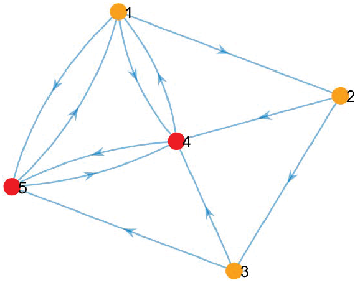
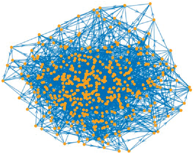
In this section, we test the privacy and convergence performances of PPSD in two practical problems. Here, we constructed two networks with 5 and 500 nodes, respectively, for simulations, see Fig. 2.
Refer to caption
(a) 𝒢1\mathcal{G}_{1}
Refer to caption
(b) 𝒢2\mathcal{G}_{2}
Fig. 2: Networks with 55 agents (a) and 500500 agents (b).

VI-A Privacy Preservation in the Rendezvous Problem

In this problem, the task of each agent ii is to collaborate with other agents to find the nearest rendezvous point without revealing its initial position 𝐩i∈ℝd\mathbf{p}_{i}\in\mathbb{R}^{d}. Each fif_{i} of the rendezvous problem is modeled as fi​(𝐱)=12​∥𝐱−𝐩i∥2f_{i}(\mathbf{x})=\frac{1}{2}\lVert\mathbf{x}-\mathbf{p}_{i}\rVert^{2}.

We set d=1d=1 and choose the network 𝒢1\mathcal{G}_{1} as shown in Fig. 2(a). Let agents 44 and 55 be corrupted agents, i.e., 𝒜={4,5}\mathcal{A}=\{4,5\}, which try to infer the gradient information of normal agent 11, and agent 22 be a normal out-neighbor of agent 11. Note that agent 44 and agent 55 can collude with each other. In this experiment, we first run PPSD once and record the accessible information to the corrupted agents ℐ𝒜={ℐ4(k)∪ℐ5(k)|k=0,1⋯}\mathcal{I}_{\mathcal{A}}=\{\mathcal{I}_{4}(k)\cup\mathcal{I}_{5}(k)\left|k=0,1\cdots\right.\}. Then, we show that the information accessed by the corrupted agents, denoted by ℐ~𝒜\tilde{\mathcal{I}}_{\mathcal{A}}, under the gradient ∇f~1​(𝐱~1)=∇f1​(𝐱1)+𝜹\nabla\tilde{f}_{1}(\mathbf{\tilde{x}}_{1})=\nabla f_{1}(\mathbf{x}_{1})+\bm{\delta}, where each element of 𝜹\bm{\delta} is selected from (0,5000)(0,5000) arbitrarily.

Fig. 3 shows that the gradients ∇f1​(𝐱1)\nabla f_{1}(\mathbf{x}_{1}) and ∇f~1​(𝐱~1)\nabla\tilde{f}_{1}(\mathbf{\tilde{x}}_{1}) used in the two runs of PPSD are clearly different, but the information accessible to the corrupted agents 𝒜\mathcal{A} (i.e., 𝐱1k\mathbf{x}_{1}^{k}, 𝚲1k​𝐲1,αk\mathbf{\Lambda}_{1}^{k}\mathbf{y}_{1,\alpha}^{k}, 𝐂41k​𝐲1,αk\mathbf{C}_{41}^{k}\mathbf{y}_{1,\alpha}^{k}, 𝐂51k​𝐲1,αk\mathbf{C}_{51}^{k}\mathbf{y}_{1,\alpha}^{k} in ℐ𝒜\mathcal{I}_{\mathcal{A}} and 𝐱~1k\mathbf{\tilde{x}}_{1}^{k}, 𝚲~1k​𝐲~1,αk\mathbf{\tilde{\Lambda}}_{1}^{k}\mathbf{\tilde{y}}_{1,\alpha}^{k}, 𝐂~41k​𝐲~1,αk\mathbf{\tilde{C}}_{41}^{k}\mathbf{\tilde{y}}_{1,\alpha}^{k}, 𝐂~51k​𝐲~1,αk\mathbf{\tilde{C}}_{51}^{k}\mathbf{\tilde{y}}_{1,\alpha}^{k} in ℐ~𝒜\tilde{\mathcal{I}}_{\mathcal{A}}) is exactly the same as shown in Fig. 4. Therefore, the corrupted agents 𝒜\mathcal{A} are unable to infer which is the true gradient information of normal agent 11.

Refer to caption
Fig. 3: Two different gradients of agent 11.
Refer to caption
Refer to caption
Fig. 4: The information accessible to corrupted agents 44 and 55 are the same under two different gradients of agent 11 shown in Fig. 3.

VI-B Decentralized Linear Regression

We show the convergence performances of PPSD in the decentralized linear regression problem, where each agent collaborates with each other to estimate an unknown signal 𝐬0∈ℝd\mathbf{s}_{0}\in\mathbb{R}^{d}. Specifically, each agent grasps a measurement relation 𝐦i=𝑸i​𝐬0+𝜻i\mathbf{m}_{i}=\bm{Q}_{i}\mathbf{s}_{0}+\bm{\zeta}_{i}, in which 𝑸i∈ℝpi×d\bm{Q}_{i}\in\mathbb{R}^{p_{i}\times d} is an observation matrix and 𝜻i∈ℝpi\bm{\zeta}_{i}\in\mathbb{R}^{p_{i}} is an interfering noise. Each fif_{i} of the linear regression problem is modeled as fi​(𝐱)=∥𝑸i​𝐱−𝐦i∥2f_{i}(\mathbf{x})=\lVert\bm{Q}_{i}\mathbf{x}-\mathbf{m}_{i}\rVert^{2}.

We set d=10d=10 and pi=10p_{i}=10 for all i∈𝒱i\in\mathcal{V}, and choose the network 𝒢1\mathcal{G}_{1}. Let each element of 𝐬0\mathbf{s}_{0} and 𝜻i\bm{\zeta}_{i} be i.i.d. random value drawn from 𝒩⁡(0,1)\mathcal{N}(0,1) and 𝒩⁡(0,0.2)\mathcal{N}(0,0.2), respectively. We fix 𝑸i\bm{Q}_{i} with each element being i.i.d. random value drawn from 𝒩⁡(0,1)\mathcal{N}(0,1) and then normalize the matrix. The residual ∥𝐱k−𝟏n⊗𝐱∗∥\lVert\mathbf{x}^{k}-\mathbf{1}_{n}\otimes\mathbf{x}^{\ast}\rVert is used as the performance metric.

Comparison with Decentralized Optimization Algorithms. We compare PPSD with Push-Pull [18], 𝒜​ℬ\mathcal{A}\mathcal{B} [13], Push-DIGing [9], ADD-OPT [10], and Subgradient-Push [20] to verify the impact of security mechanisms on convergence accuracy. As shown in Fig. 5, PPSD achieves a linear convergence rate and the place marked in the curve indicates that the randomness added to the corresponding parameters prolongs the convergence process.

Refer to caption
Fig. 5: Performance comparison.

Comparison with [26]. We compare PPSD with the differential privacy based algorithm [26]. We consider the performance of the algorithm [26] under four privacy levels, i.e., σ=10−6,10−4,10−2,1\sigma=10^{-6},10^{-4},10^{-2},1, where σ\sigma is the scale parameter. Note that a larger σ\sigma means a greater privacy level. From Fig. 6, one can see that the differential privacy based algorithm [26] has a compromise between convergence accuracy and privacy level, and also demonstrates the advantages of PPSD in ensuring convergence accuracy.

Refer to caption
Fig. 6: Performance comparison.

Comparison with [34]. We compare PPSD with the dynamics based privacy-preserving algorithm [34]. The main idea of the algorithm in [34] to achieve privacy preservation is to add randomness to the mixing matrix in the first KK iterations. Here, we consider four cases: K=1,2,3,4K=1,2,3,4. As depicted in Fig. 7, the randomness added in the first KK iterations in [34] has no impact on the convergence rate, but there is a significant decay in the convergence accuracy. Although PPSD converges slightly slower than the algorithm [34], it ensures a higher convergence accuracy.

Refer to caption
Fig. 7: Performance comparison.

Simulation on the Large-scale Network. Finally, we use 𝒢2\mathcal{G}_{2} to check the scalability of PPSD. Other settings are the same as the above. It is shown in Fig. 8 that PPSD achieves a linear convergence rate even in large-scale networks.

Refer to caption
Fig. 8: The performance on 𝒢2\mathcal{G}_{2}.

VII Conclusion

We proposed a novel privacy-preserving decentralized optimization algorithm (PPSD) via state decomposition for unbalanced digraphs. Compared to algorithms based on differential privacy or homomorphic encryption, PPSD ensures convergence performance without incurring additional computational burden. We critically analyzed the convergence rate and privacy performance of PPSD and further verified it in simulation experiments. Future work will continually focus on the design of privacy mechanisms for decentralized algorithms.

References

  • [1] K. Anastasiia, T. Lin, and S. U. Stich, “An improved analysis of gradient tracking for decentralized machine learning,” in Proc. Adv. Neural Inf. Process. Syst., vol. 34, pp. 11422–11435, 2021.
  • [2] H. J. Liu, W. Shi, and H. Zhu, “Decentralized dynamic optimization for power network voltage control,” IEEE Trans. Signal Inform. Process. Over Netw., vol 3, no.3, pp. 568–579, 2016.
  • [3] J. Zhang, K. You, and K. Cai, “Distributed dual gradient tracking for resource allocation in unbalanced networks,” IEEE Trans. Signal Proces., vol. 68, pp. 2186–2198, 2020
  • [4] Y. Xu, T. Han, K. Cai, Z Lin, G. Yan, and M. Fu, “A distributed algorithm for resource allocation over dynamic digraphs,” IEEE Trans. Signal Proces., vol. 65, no. 10, pp. 2600–2612, 2017
  • [5] A. Nedić and A. Ozdaglar, “Distributed subgradient methods for multi-agent optimization,” IEEE Trans. Autom. Control, vol. 54, no. 1, pp. 48–61, 2009.
  • [6] J. Xu, S. Zhu, Y. C. Soh, and L. Xie, “Augmented distributed gradient methods for multi-agent optimization under uncoordinated constant stepsizes,” in Proc. IEEE 54th Conf. Decis. Control, pp. 2055–2060, 2015.
  • [7] J. Xu, S. Zhu, Y. C. Soh, and L. Xie, “Convergence of asynchronous distributed gradient methods over stochastic networks,” IEEE Trans. Autom. Control, vol. 63, no. 2, pp. 434–448, 2017.
  • [8] G. Qu and N. Li, “Harnessing smoothness to accelerate distributed optimization,” IEEE Trans. Control Netw. Syst., vol. 5, no. 3, pp. 1245–1260, 2017.
  • [9] A. Nedić, A. Olshevsky, and W. Shi, “Achieving geometric convergence for distributed optimization over time-varying graphs,” SIAM J. Optim., vol. 27, no.4, pp. 2597–2633, 2017.
  • [10] C. Xi, R. Xin, and U. A. Khan, “ADD-OPT: Accelerated distributed directed optimization,” IEEE Trans. Autom. Control, vol. 63, no. 5, pp. 1329–1339, 2017.
  • [11] Y. Sun, G. Scutari, and D. Palomar, “Distributed nonconvex multiagent optimization over time-varying networks,” in Proc. 50th Asilomar Conf. Signals, Syst. Comput., pp. 788–794, 2016.
  • [12] Y. Tian, Y. Sun, and G. Scutari, “Achieving linear convergence in distributed asynchronous multiagent optimization,” IEEE Trans. Autom. Control, vol. 65, no. 12, pp. 5264–5279, 2020.
  • [13] R. Xin and U. A. Khan, “A linear algorithm for optimization over directed graphs with geometric convergence,” IEEE Control Syst. Lett., vol. 2, no. 3, pp. 325–330, 2018.
  • [14] F. Saadatniaki, R. Xin, and U. A. Khan, “Decentralized optimization over time-varying directed graphs with row and column-stochastic matrices,” IEEE Trans. Autom. Control, vol. 65, no. 11, pp. 4769–4780, 2020.
  • [15] A. Nedić, D. T. A. Nguyen, and D. T. Nguyen, “AB/Push-Pull Method for Distributed Optimization in Time-Varying Directed Networks,” arXiv preprint arXiv:2209.06974, 2022.
  • [16] W. Du, L. Yao, D. Wu, X. Li, G. Liu, and T. Yang, “Accelerated distributed energy management for microgrids,” in Proc. IEEE Power Energy Soc. Gen. Meeting, pp. 1–5, 2018.
  • [17] S. Zhang, X. Yi, J. George, and T. Yang, “Computational convergence analysis of distributed optimization algorithms for directed graphs,” in Proc. IEEE 15th Int. Conf. Control Autom., pp. 1096–1101, 2019.
  • [18] S. Pu, W. Shi, J. Xu, and A. Nedić, “Push-pull gradient methods for distributed optimization in networks,” IEEE Trans. Autom. Control, vol. 66, no. 1, pp. 1–16, Jan. 2021.
  • [19] W. Shi, Q. Ling, G. Wu, and W. Yin, “EXTRA: An exact first-order algorithm for decentralized consensus optimization,” SIAM J. Optim., vol. 25, no. 2, pp. 944–966, 2014.
  • [20] A. Nedić and A. Olshevsky, “Distributed optimization over time-varying directed graphs,” IEEE Trans. Autom. Control, vol. 60, no. 3, pp. 601–615, Mar. 2015.
  • [21] J. Zhang and K. You, “AsySPA: An exact asynchronous algorithm for convex optimization over digraphs,” IEEE Trans. Autom. Control, vol. 65, no. 6, pp. 2494–2509, 2020.
  • [22] Z. Huang, S. Mitra, and N. Vaidya, “Differentially private distributed optimization,” in Proc. Int. Conf. Distrib. Comput. Netw., 2015, pp. 4:1–4:10.
  • [23] F. Yan, S. Sundaram, S. V. N. Vishwanathan, and Y. Qi, “Distributed autonomous online learning: Regrets and intrinsic privacy-preserving properties,” IEEE Trans. Knowl. Data Eng., vol. 25, no. 11, pp. 2483–2493, 2012.
  • [24] Y. Wang and A. Nedić, “Tailoring gradient methods for differentially private distributed optimization,” IEEE Trans. Autom. Control, doi: 10.1109/TAC.2023.3272968, 2023.
  • [25] T. Ding, S. Zhu, J. He, C. Chen, and X. Guan, “Differentially private distributed optimization via state and direction perturbation in multiagent systems,” IEEE Trans. Autom. Control, vol. 67, no. 2, 722-737, 2021.
  • [26] X. Chen, L. Huang, L. He, S. Dey, and L. Shi, “A differentially private method for distributed optimization in directed networks via state decomposition,” IEEE Trans. Control Netw. Syst., doi: 10.1109/TCNS.2023.3264932, 2023.
  • [27] Y. Lu and M. Zhu, “Privacy preserving distributed optimization using homomorphic encryption,” Automatica, vol. 96, pp. 314–325, 2018.
  • [28] C. Zhang, M. Ahmad, and Y. Wang, “ADMM based privacy preserving decentralized optimization,” IEEE Trans. Inf. Forensic Secur, vol. 14, no. 3, pp. 565–580, 2018.
  • [29] C. Zhang and Y. Wang, “Enabling privacy-preservation in decentralized optimization,” IEEE Trans. Control Netw. Syst., vol. 6, no. 2, pp. 679–689, 2018.
  • [30] Y. Lou, L. Yu, S. Wang, and P. Yi, “Privacy preservation in distributed subgradient optimization algorithms,” IEEE Trans. Cybern., vol. 48, no. 7, pp. 2154–2165, 2018.
  • [31] S. Gade and N. H. Vaidya, “Private optimization on networks,” in Proc. 2018 American Control Conf., pp. 1402–1409, 2018.
  • [32] Q. Li, R. Heusdens, and M. G. Christensen, “Privacy-preserving distributed optimization via subspace perturbation: A general framework,” IEEE Trans. Signal Proces., vol. 68, pp. 5983–5996, 2020.
  • [33] Y. Wang and V. Poor, “Decentralized stochastic optimization with inherent privacy protection,” IEEE Trans. Autom. Control, vol. 68, no. 4, pp. 2293–2308, 2022.
  • [34] H. Gao, Y. Wang, and A. Nedić, “Dynamics based privacy preservation in decentralized optimization,” Automatica, vol. 151, pp. 110878, 2023.
  • [35] T. Charalambous, N. E. Manitara, and C. N. Hadjicostis, “Privacy-preserving average consensus over digraphs in the presence of time delays,” In Proc. 57th Annu. Allerton Conf. Commun. Control Comput., pp. 238–245, 2019.
  • [36] H. Gao, C. Zhang, M. Ahmad, and Y. Wang, “Privacy-preserving average consensus on directed graphs using push-sum,” In Proc. IEEE Conf. Commun. Netw. Security, pp. 1–9, 2018.
  • [37] Y. Mo and R. M. Murray, “Privacy preserving average consensus,” IEEE Trans. Autom. Control, vol. 62, no. 2, pp. 753–765, 2017.
  • [38] M. Ruan, H. Gao, and Y. Wang, “Secure and privacy-preserving consensus,” IEEE Trans. Autom. Control, vol. 64, no. 10, pp. 4035–4049, Oct. 2019.
  • [39] Y. Wang, “Privacy-preserving average consensus via state decomposition,” IEEE Trans. Autom. Control, vol. 64, no. 11, pp. 4711–4716, 2019.
  • [40] X. Chen, L. Huang, K. Ding, S. Dey, and L. Shi, “Privacy-preserving push-sum average consensus via state decomposition,” IEEE Trans. Autom. Control, doi:10.1109/TAC.2023.3256479, 2023.
  • [41] H. Gao, and Y. Wang, “Algorithm-level confidentiality for average consensus on time-varying directed graphs,” IEEE Trans. Netw. Sci. Eng., vol. 9, no. 2, pp. 918–931, 2022.
  • [42] A. Alaeddini, K. Morgansen, and M. Mesbah, “Adaptive communication networks with privacy guarantees,” in Proc. 2017 American Contr. Conf., pp. 4460–4465, 2017.
  • [43] S. Pequito, S. Kar, S. Sundaram, and A. P. Aguiar, “Design of communication networks for distributed computation with privacy guarantees,” in Proc. IEEE 53rd Conf. Decis. Control, pp. 1370–1376, 2014.
  • [44] D. Lefebvre and C. N. Hadjicostis, “Privacy and safety analysis of timed stochastic discrete event systems using markovian trajectoryobservers,” Discret. Event Dyn. Syst., vol. 30, no. 3, pp. 413–440, 2020.
  • [45] A. Saboori and C. N. Hadjicostis, “Verification of initial-state opacity in security applications of discrete event systems,” Inform. Sciences, vol. 246, pp. 115–132, 2013.
  • [46] B. Ramasubramanian, W. R. Cleaveland, and S. Marcus, “Notions of centralized and decentralized opacity in linear systems,” IEEE Trans. Autom. Control, vol. 65, no. 4, pp. 1442–1455, 2019.
  • [47] E. Seneta, “Non-negative matrices and Markov chains,” Springer Science & Business Media, 2006.
  • [48] A. Nedić and J. Liu, “On convergence rate of weighted-averaging dynamics for consensus problems,” IEEE Trans. Autom. Control, vol. 62, no. 2, pp. 766–781, 2016.
  • [49] P. D. Powell, “Calculating determinants of block matrices,” arXiv preprint arXiv:1112.4379, 2011.
  • [50] R. A. Horn and C. R. Johnson, “Matrix analysis,” Cambridge university press, 2012.

Appendix A Proof of Lemma 4

Proof.

By the dynamics (10), it follows for k≥N¯k\geq\bar{N}:

𝐱k+1=\displaystyle\mathbf{x}^{k+1}= 𝐑k:k−N¯+1𝐱k−N¯+1\displaystyle\mathbf{R}_{k:k-\bar{N}+1}\mathbf{x}^{k-\bar{N}+1}
−γ(𝐀k𝐓𝐲k+∑l=1N¯−1𝐑k:k−l+1𝐀k−l𝐓𝐲k−l)\displaystyle-\gamma\Big(\mathbf{A}^{k}\mathbf{Ty}^{k}+\sum_{l=1}^{\bar{N}-1}{\mathbf{R}_{k:k-l+1}\mathbf{A}^{k-l}\mathbf{Ty}^{k-l}}\Big)

Then, for 𝐱~wk+1\mathbf{\tilde{x}}_{\text{w}}^{k+1}, it holds

∥𝐱~wk+1∥\displaystyle\lVert\mathbf{\tilde{x}}_{\text{w}}^{k+1}\rVert
≤\displaystyle\leq ∥[(𝐈n−𝟏n(ϕk+1)⊤)⊗𝐈d]𝐑k:k−N¯+1𝐱k−N¯+1∥\displaystyle\lVert[(\mathbf{I}_{n}-\mathbf{1}_{n}(\bm{\phi}^{k+1})^{\top})\otimes\mathbf{I}_{d}]\mathbf{R}_{k:k-\bar{N}+1}\mathbf{x}^{k-\bar{N}+1}\rVert
+γ⁡∥[(𝐈n−𝟏n​(ϕk+1)⊤)⊗𝐈d]​𝐀k​𝐓𝐲k∥\displaystyle+\gamma\lVert[(\mathbf{I}_{n}-\mathbf{1}_{n}(\bm{\phi}^{k+1})^{\top})\otimes\mathbf{I}_{d}]\mathbf{A}^{k}\mathbf{Ty}^{k}\rVert
+γ∑l=1N¯−1∥[(𝐈n−𝟏n(ϕk+1)⊤)⊗𝐈d]𝐑k:k−l+1𝐀k−l𝐓𝐲k−l∥\displaystyle+\!\gamma\sum_{l=1}^{\bar{N}-1}{\lVert[(\mathbf{I}_{n}\!-\!\mathbf{1}_{n}(\bm{\phi}^{k+1})^{\top})\!\otimes\!\mathbf{I}_{d}]\mathbf{R}_{k:k-l+1}\mathbf{A}^{k-l}\mathbf{Ty}^{k-l}\rVert}
≤\displaystyle\,\,\leq rR​∥[(𝐈n−𝟏n​(ϕk−N¯+1)⊤)⊗𝐈d]​𝐱k−N¯+1∥+γ​QR​n​∥𝐲k∥\displaystyle r_{R}\lVert[(\mathbf{I}_{n}\!-\!\mathbf{1}_{n}(\bm{\phi}^{k-\bar{N}+1})^{\top})\!\otimes\!\mathbf{I}_{d}]\mathbf{x}^{k-\bar{N}+1}\rVert\!+\!\gamma Q_{R}\sqrt{n}\lVert\mathbf{y}^{k}\rVert
+γ∑l=1N¯−1∥[(𝐈n−𝟏n(ϕk−l+1)⊤)⊗𝐈d]𝐀k−l𝐓𝐲k−l∥\displaystyle+\gamma\sum_{l=1}^{\bar{N}-1}{\lVert[(\mathbf{I}_{n}-\mathbf{1}_{n}(\bm{\phi}^{k-l+1})^{\top})\otimes\mathbf{I}_{d}]\mathbf{A}^{k-l}\mathbf{Ty}^{k-l}\rVert}
≤\displaystyle\,\,\leq rR​∥𝐱~wk−N¯+1∥+γ​QR​n​∑l=0N¯−1∥𝐲k−l∥,\displaystyle r_{R}\lVert\mathbf{\tilde{x}}_{\text{w}}^{k-\bar{N}+1}\rVert+\gamma Q_{R}\sqrt{n}\sum_{l=0}^{\bar{N}-1}{\lVert\mathbf{y}^{k-l}\rVert}, (A2)

where the second inequality uses that ∥𝐈n−𝟏n​(ϕk−N¯+1)⊤∥≤2​n\lVert\mathbf{I}_{n}-\mathbf{1}_{n}(\bm{\phi}^{k-\bar{N}+1})^{\top}\rVert\leq 2\sqrt{n}, ∥𝐀k∥≤n\lVert\mathbf{A}^{k}\rVert\leq\sqrt{n}, 2​n≤QR2\sqrt{n}\leq Q_{R}, ∥𝐓∥=1\lVert\mathbf{T}\rVert=1, and N¯=max⁡{NR,NP}\bar{N}=\max\{N_{R},N_{P}\}. Next, we analyze ∥𝐲k∥\lVert\mathbf{y}^{k}\rVert. From the dynamic of (11), we have

(𝟏n~​(𝐯k)⊤⊗𝐈d)​𝐬k\displaystyle(\mathbf{1}_{\tilde{n}}(\mathbf{v}^{k})^{\top}\otimes\mathbf{I}_{d})\mathbf{s}^{k}
=\displaystyle= (𝟏n~​(𝐯k−1)⊤⊗𝐈d)​𝐬k−1+(𝟏n~​𝟏n~⊤⊗𝐈d)​(∇𝐟^​(𝐱k)−∇𝐟^​(𝐱k−1))\displaystyle(\mathbf{1}_{\tilde{n}}(\mathbf{v}^{k-1})^{\top}\!\otimes\!\mathbf{I}_{d})\mathbf{s}^{k-1}\!+\!(\mathbf{1}_{\tilde{n}}\mathbf{1}_{\tilde{n}}^{\top}\!\otimes\!\mathbf{I}_{d})(\nabla\mathbf{\hat{f}}(\mathbf{x}^{k})\!-\!\nabla\mathbf{\hat{f}}(\mathbf{x}^{k-1}))
=\displaystyle= (𝟏n~​(𝐯1)⊤⊗𝐈d)​𝐬1+(𝟏n~​𝟏n~⊤⊗𝐈d)​(∇𝐟^​(𝐱k)−∇𝐟^​(𝐱1))\displaystyle(\mathbf{1}_{\tilde{n}}(\mathbf{v}^{1})^{\top}\otimes\mathbf{I}_{d})\mathbf{s}^{1}+(\mathbf{1}_{\tilde{n}}\mathbf{1}_{\tilde{n}}^{\top}\otimes\mathbf{I}_{d})(\nabla\mathbf{\hat{f}}(\mathbf{x}^{k})-\nabla\mathbf{\hat{f}}(\mathbf{x}^{1}))
=\displaystyle= (𝟏n~𝟏n~⊤⊗𝐈d)(𝐲1−∇𝐟^(𝐱1))+(𝟏n~𝟏n~⊤⊗𝐈d)∇𝐟^(𝐱k)\displaystyle(\mathbf{1}_{\tilde{n}}\mathbf{1}_{\tilde{n}}^{\top}\otimes\mathbf{I}_{d})(\mathbf{y}^{1}-\nabla\mathbf{\hat{f}}(\mathbf{x}^{1}))+(\mathbf{1}_{\tilde{n}}\mathbf{1}_{\tilde{n}}^{\top}\otimes\mathbf{I}_{d})\nabla\mathbf{\hat{f}}(\mathbf{x}^{k})
=\displaystyle= (𝟏n~𝟏n~⊤⊗𝐈d)∇𝐟^(𝐱k)=(𝟏n𝟏n⊤⊗𝐈d)∇𝐟(𝐱k),\displaystyle(\mathbf{1}_{\tilde{n}}\mathbf{1}_{\tilde{n}}^{\top}\otimes\mathbf{I}_{d})\nabla\mathbf{\hat{f}}(\mathbf{x}^{k})=(\mathbf{1}_{n}\mathbf{1}_{n}^{\top}\otimes\mathbf{I}_{d})\nabla\mathbf{f}(\mathbf{x}^{k}),

where the last third relation holds since (𝟏n~​(𝐯1)⊤⊗𝐈d)​𝐬1=(𝟏n~​(𝐯1)⊤​(𝐕¯1)−1⊗𝐈d)​𝐲1=(𝟏n~​𝟏n~⊤⊗𝐈d)​𝐲1(\mathbf{1}_{\tilde{n}}(\mathbf{v}^{1})^{\top}\otimes\mathbf{I}_{d})\mathbf{s}^{1}=(\mathbf{1}_{\tilde{n}}(\mathbf{v}^{1})^{\top}(\mathbf{\bar{V}}^{1})^{-1}\otimes\mathbf{I}_{d})\mathbf{y}^{1}=(\mathbf{1}_{\tilde{n}}\mathbf{1}_{\tilde{n}}^{\top}\otimes\mathbf{I}_{d})\mathbf{y}^{1}. From the definition of 𝐬~𝐰k\mathbf{\tilde{s}}_{\mathbf{w}}^{k} and the optimality condition ∑i=1n∇fi​(𝐱∗)=𝟎d\sum\nolimits_{i=1}^{n}{\nabla f_{i}(\mathbf{x}^{\ast})}=\mathbf{0}_{d}, we obtain

𝐬k=\displaystyle\mathbf{s}^{k}= 𝐬~wk+(𝟏n~​(𝐯k)⊤⊗𝐈d)​𝐬k\displaystyle\mathbf{\tilde{s}}_{\text{w}}^{k}+(\mathbf{1}_{\tilde{n}}(\mathbf{v}^{k})^{\top}\otimes\mathbf{I}_{d})\mathbf{s}^{k}
=\displaystyle\,\,= 𝐬~wk+(𝟏n𝟏n⊤⊗𝐈d)∇𝐟(𝐱k)\displaystyle\mathbf{\tilde{s}}_{\text{w}}^{k}+(\mathbf{1}_{n}\mathbf{1}_{n}^{\top}\otimes\mathbf{I}_{d})\nabla\mathbf{f}(\mathbf{x}^{k})
=\displaystyle\,\,= 𝐬~wk+(𝟏n​𝟏n⊤⊗𝐈d)​(∇𝐟​(𝐱k)−∇𝐟​(𝟏n⊗𝐱∗)).\displaystyle\mathbf{\tilde{s}}_{\text{w}}^{k}+(\mathbf{1}_{n}\mathbf{1}_{n}^{\top}\otimes\mathbf{I}_{d})(\nabla\mathbf{f}(\mathbf{x}^{k})-\nabla\mathbf{f}(\mathbf{1}_{n}\otimes\mathbf{x}^{\ast})).

Thus, we bound 𝐬k\mathbf{s}^{k} as

∥𝐬k∥≤\displaystyle\lVert\mathbf{s}^{k}\rVert\leq ∥𝐬~wk∥+n​L​∥𝐱k−𝟏n⊗𝐱∗∥\displaystyle\lVert\mathbf{\tilde{s}}_{\text{w}}^{k}\rVert+nL\lVert\mathbf{x}^{k}-\mathbf{1}_{n}\otimes\mathbf{x}^{\ast}\rVert
≤\displaystyle\leq ∥𝐬~wk∥+n​L​∥𝐱k−(𝟏n​(ϕk)⊤⊗𝐈d)​𝐱k∥\displaystyle\lVert\mathbf{\tilde{s}}_{\text{w}}^{k}\rVert+nL\lVert\mathbf{x}^{k}-(\mathbf{1}_{n}(\bm{\phi}^{k})^{\top}\otimes\mathbf{I}_{d})\mathbf{x}_{k}\rVert
+n​L​∥(𝟏n​(ϕk)⊤⊗𝐈d)​𝐱k−𝟏n⊗𝐱∗∥\displaystyle+nL\lVert(\mathbf{1}_{n}(\bm{\phi}^{k})^{\top}\otimes\mathbf{I}_{d})\mathbf{x}_{k}-\mathbf{1}_{n}\otimes\mathbf{x}^{\ast}\rVert
≤\displaystyle\leq ∥𝐬~wk∥+n​L​∥𝐱~𝐰k∥+n​L​∥𝐫k∥.\displaystyle\lVert\mathbf{\tilde{s}}_{\text{w}}^{k}\rVert+nL\lVert\mathbf{\tilde{x}}_{\mathbf{w}}^{k}\rVert+nL\lVert\mathbf{r}^{k}\rVert. (A3)

Since 𝐬k=((𝐕¯k)−1⊗𝐈d)​𝐲k\mathbf{s}^{k}=((\mathbf{\bar{V}}^{k})^{-1}\otimes\mathbf{I}_{d})\mathbf{y}^{k}, it holds 𝐲k=(𝐕¯k⊗𝐈d)​𝐬k\mathbf{y}^{k}=(\mathbf{\bar{V}}^{k}\otimes\mathbf{I}_{d})\mathbf{s}^{k}. Further, using the relation ∥𝐕¯k∥=maxi⁡[𝐯k]i<1\lVert\mathbf{\bar{V}}^{k}\rVert=\max_{i}[\mathbf{v}_{k}]_{i}<1 gives

∥𝐲k∥≤∥𝐕¯k∥​∥𝐬k∥≤∥𝐬k∥.\displaystyle\lVert\mathbf{y}^{k}\rVert\leq\lVert\mathbf{\bar{V}}^{k}\rVert\lVert\mathbf{s}^{k}\rVert\leq\lVert\mathbf{s}^{k}\rVert. (A4)

Substituting the results of (A3) and (A4) into (A2) completes the proof. ∎

Appendix B Proof of Lemma 5

Proof.

It is easily verified from the definitions of 𝐱¯wk\mathbf{\bar{x}}_{\text{w}}^{k} and 𝐫k\mathbf{r}^{k} that 𝐫k=(𝟏n​(ϕk)⊤⊗𝐈d)​𝐱k−𝟏n⊗𝐱∗\mathbf{r}^{k}=(\mathbf{1}_{n}(\bm{\phi}^{k})^{\top}\otimes\mathbf{I}_{d})\mathbf{x}^{k}-\mathbf{1}_{n}\otimes\mathbf{x}^{\ast}. Then, using the dynamic (10) gives

𝐫k+1=\displaystyle\mathbf{r}^{k+1}= (𝟏n​(ϕk+1)⊤⊗𝐈d)​𝐑k​𝐱k−𝟏n⊗𝐱∗\displaystyle(\mathbf{1}_{n}(\bm{\phi}^{k+1})^{\top}\otimes\mathbf{I}_{d})\mathbf{R}^{k}\mathbf{x}^{k}-\mathbf{1}_{n}\otimes\mathbf{x}^{\ast}
−γ⁡(𝟏n​(ϕk+1)⊤⊗𝐈d)​𝐀k​𝐓𝐲k\displaystyle-\gamma(\mathbf{1}_{n}(\bm{\phi}^{k+1})^{\top}\otimes\mathbf{I}_{d})\mathbf{A}^{k}\mathbf{Ty}^{k}
=\displaystyle= (𝟏n​(ϕk)⊤⊗𝐈d)​𝐱k−𝟏n⊗𝐱∗\displaystyle(\mathbf{1}_{n}(\bm{\phi}^{k})^{\top}\otimes\mathbf{I}_{d})\mathbf{x}^{k}-\mathbf{1}_{n}\otimes\mathbf{x}^{\ast}
−γ⁡[(𝟏n​(ϕk+1)⊤​𝐀¯k​𝐓¯​𝐯k​𝟏n~⊤)⊗𝐈d]​𝐲k\displaystyle-\gamma[(\mathbf{1}_{n}(\bm{\phi}^{k+1})^{\top}\mathbf{\bar{A}}^{k}\mathbf{\bar{T}v}^{k}\mathbf{1}_{\tilde{n}}^{\top})\otimes\mathbf{I}_{d}]\mathbf{y}^{k}
−γ⁡(𝟏n​(ϕk+1)⊤⊗𝐈d)​𝐀k​𝐓​(𝐲k−(𝐯k​𝟏n~⊤⊗𝐈d)​𝐲k).\displaystyle-\gamma(\mathbf{1}_{n}(\bm{\phi}^{k+1})^{\top}\otimes\mathbf{I}_{d})\mathbf{A}^{k}\mathbf{T}(\mathbf{y}^{k}-(\mathbf{v}^{k}\mathbf{1}_{\tilde{n}}^{\top}\otimes\mathbf{I}_{d})\mathbf{y}^{k}).

We bound 𝐫k+1\mathbf{r}^{k+1} as

∥𝐫k+1∥\displaystyle\lVert\mathbf{r}^{k+1}\rVert
≤\displaystyle\leq ‖(𝟏n(ϕk)⊤⊗𝐈d)𝐱k−𝟏n⊗𝐱∗\displaystyle\left\|(\mathbf{1}_{n}(\bm{\phi}^{k})^{\top}\otimes\mathbf{I}_{d})\mathbf{x}^{k}-\mathbf{1}_{n}\otimes\mathbf{x}^{\ast}\right.
−γ[(𝟏n(ϕk+1)⊤𝐀¯k𝐓¯𝐯k𝟏n~⊤)⊗𝐈d]𝐲k‖\displaystyle\,\,\left.-\gamma[(\mathbf{1}_{n}(\bm{\phi}^{k+1})^{\top}\mathbf{\bar{A}}^{k}\mathbf{\bar{T}v}^{k}\mathbf{1}_{\tilde{n}}^{\top})\otimes\mathbf{I}_{d}]\mathbf{y}^{k}\right\|
+∥γ⁡(𝟏n​(ϕk+1)⊤⊗𝐈d)​𝐀k​𝐓​(𝐲k−(𝐯k​𝟏n~⊤⊗𝐈d)​𝐲k)∥\displaystyle+\lVert\gamma(\mathbf{1}_{n}(\bm{\phi}^{k+1})^{\top}\otimes\mathbf{I}_{d})\mathbf{A}^{k}\mathbf{T}(\mathbf{y}^{k}-(\mathbf{v}^{k}\mathbf{1}_{\tilde{n}}^{\top}\otimes\mathbf{I}_{d})\mathbf{y}^{k})\rVert
≤\displaystyle\leq ∥(𝟏n​(ϕk)⊤⊗𝐈d)​𝐱k−𝟏n⊗𝐱∗−γ​ϱk​[(𝟏n​𝟏n~⊤)⊗𝐈d]​𝐲k∥\displaystyle\lVert(\mathbf{1}_{n}(\bm{\phi}^{k})^{\top}\otimes\mathbf{I}_{d})\mathbf{x}^{k}-\mathbf{1}_{n}\otimes\mathbf{x}^{\ast}-\gamma\varrho^{k}[(\mathbf{1}_{n}\mathbf{1}_{\tilde{n}}^{\top})\otimes\mathbf{I}_{d}]\mathbf{y}^{k}\rVert
+γ​n​∥𝐬~wk∥,\displaystyle+\gamma n\lVert\mathbf{\tilde{s}}_{\text{w}}^{k}\rVert, (A5)

where ϱk≔(ϕk+1)⊤​𝐀¯k​𝐓¯​𝐯k∈ℝ\varrho^{k}\coloneqq(\bm{\phi}^{k+1})^{\top}\mathbf{\bar{A}}^{k}\mathbf{\bar{T}v}^{k}\in\mathbb{R}, and the last inequality uses the relations that ∥𝟏n​(ϕk)⊤⊗𝐈d∥≤n\lVert\mathbf{1}_{n}(\bm{\phi}^{k})^{\top}\otimes\mathbf{I}_{d}\rVert\leq\sqrt{n}, ∥𝐀k∥≤n\lVert\mathbf{A}^{k}\rVert\leq\sqrt{n}, 𝐲k−(𝐯k​𝟏n~⊤⊗𝐈d)​𝐲k=(𝐕¯k⊗𝐈d)​𝐬~wk\mathbf{y}^{k}-(\mathbf{v}^{k}\mathbf{1}_{\tilde{n}}^{\top}\otimes\mathbf{I}_{d})\mathbf{y}^{k}=(\mathbf{\bar{V}}^{k}\otimes\mathbf{I}_{d})\mathbf{\tilde{s}}_{\text{w}}^{k}, and ∥𝐕¯k⊗𝐈d∥≤1\lVert\mathbf{\bar{V}}^{k}\otimes\mathbf{I}_{d}\rVert\leq 1. Note that vik∈[ηn~−1/n~,1]v_{i}^{k}\in[\eta^{\tilde{n}-1}/\tilde{n},1] for k≥1k\geq 1 [14, 34]. Using the row stochasticity of 𝐀¯k\mathbf{\bar{A}}^{k}, i.e., ∑j=1nai​jk=1\sum\nolimits_{j=1}^{n}{a_{ij}^{k}}=1, yields ηn~−1/n~≤∑j=1nai​jk​vjk≤1\eta^{\tilde{n}-1}/\tilde{n}\leq\sum\nolimits_{j=1}^{n}{a_{ij}^{k}v_{j}^{k}}\leq 1 for any i=1,⋯,ni=1,\cdots,n. Thus, it follows from the relation ∑i=1nϕik+1=1\sum\nolimits_{i=1}^{n}{\phi_{i}^{k+1}}=1 that

ϱk=(ϕk+1)⊤​𝐀¯k​𝐓¯​𝐯k=∑i=1nϕik+1​∑j=1nai​jk​vjk∈[ηn~−1/n~,1],\displaystyle\varrho^{k}=(\bm{\phi}^{k+1})^{\top}\mathbf{\bar{A}}^{k}\mathbf{\bar{T}v}^{k}=\sum_{i=1}^{n}{\phi_{i}^{k+1}\sum_{j=1}^{n}{a_{ij}^{k}v_{j}^{k}}\in[\eta^{\tilde{n}-1}/\tilde{n},1]},

where the second equality uses the relation [𝐓¯​𝐯k]i=vik[\mathbf{\bar{T}v}^{k}]_{i}=v_{i}^{k} for i=1,⋯,ni=1,\cdots,n. Besides, one can verify (𝟏n~⊤⊗𝐈d)𝐲k=(𝟏n~⊤⊗𝐈d)∇𝐟~(𝐱k)=(𝟏n⊤⊗𝐈d)∇𝐟(𝐱k)(\mathbf{1}_{\tilde{n}}^{\top}\otimes\mathbf{I}_{d})\mathbf{y}^{k}=(\mathbf{1}_{\tilde{n}}^{\top}\otimes\mathbf{I}_{d})\nabla\mathbf{\tilde{f}}(\mathbf{x}^{k})=(\mathbf{1}_{n}^{\top}\otimes\mathbf{I}_{d})\nabla\mathbf{f}(\mathbf{x}^{k}). Thus, it holds

∥(𝟏n​(ϕk)⊤⊗𝐈d)​𝐱k−𝟏n⊗𝐱∗−γ​ϱk​(𝟏n​𝟏n~⊤⊗𝐈d)​𝐲k∥\displaystyle\lVert(\mathbf{1}_{n}(\bm{\phi}^{k})^{\top}\otimes\mathbf{I}_{d})\mathbf{x}^{k}-\mathbf{1}_{n}\otimes\mathbf{x}^{\ast}-\gamma\varrho^{k}(\mathbf{1}_{n}\mathbf{1}_{\tilde{n}}^{\top}\otimes\mathbf{I}_{d})\mathbf{y}^{k}\rVert
=\displaystyle= ∥𝟏n⊗𝐱¯wk−𝟏n⊗𝐱∗−γϱk(𝟏n𝟏n⊤⊗𝐈d)∇𝐟(𝐱k)∥\displaystyle\lVert\mathbf{1}_{n}\otimes\mathbf{\bar{x}}_{\text{w}}^{k}-\mathbf{1}_{n}\otimes\mathbf{x}^{\ast}-\gamma\varrho^{k}(\mathbf{1}_{n}\mathbf{1}_{n}^{\top}\otimes\mathbf{I}_{d})\nabla\mathbf{f}(\mathbf{x}^{k})\rVert
≤\displaystyle\leq ∥𝟏n⊗𝐱¯wk−𝟏n⊗𝐱∗−γϱk(𝟏n𝟏n⊤⊗𝐈d)∇𝐟(𝟏n⊗𝐱¯wk)∥\displaystyle\lVert\mathbf{1}_{n}\otimes\mathbf{\bar{x}}_{\text{w}}^{k}-\mathbf{1}_{n}\otimes\mathbf{x}^{\ast}-\gamma\varrho^{k}(\mathbf{1}_{n}\mathbf{1}_{n}^{\top}\otimes\mathbf{I}_{d})\nabla\mathbf{f}(\mathbf{1}_{n}\otimes\mathbf{\bar{x}}_{\text{w}}^{k})\rVert
+γ​ϱk​∥(𝟏n​𝟏n⊤⊗𝐈d)​(∇𝐟​(𝐱k)−∇𝐟​(𝟏n⊗𝐱¯wk))∥\displaystyle+\gamma\varrho^{k}\lVert(\mathbf{1}_{n}\mathbf{1}_{n}^{\top}\otimes\mathbf{I}_{d})(\nabla\mathbf{f}(\mathbf{x}^{k})-\nabla\mathbf{f}(\mathbf{1}_{n}\otimes\mathbf{\bar{x}}_{\text{w}}^{k}))\rVert
≤\displaystyle\leq n∥𝐱¯wk−𝐱∗−γϱk∇F(𝐱¯wk)∥+γnL∥𝐱~wk∥.\displaystyle\sqrt{n}\lVert\mathbf{\bar{x}}_{\text{w}}^{k}-\mathbf{x}^{\ast}-\gamma\varrho^{k}\nabla F(\mathbf{\bar{x}}_{\text{w}}^{k})\rVert+\gamma nL\lVert\mathbf{\tilde{x}}_{\text{w}}^{k}\rVert. (A6)

Under Assumption 2, applying Lemma 10 in [8] yields for 0<γ≤1/L¯0<\gamma\leq 1/\bar{L}

∥𝐱¯wk−𝐱∗−γϱk∇F(𝐱¯wk)∥≤1n(−γn~−1ηn~−1μ)∥𝐫k∥.\displaystyle\lVert\mathbf{\bar{x}}_{\text{w}}^{k}\!-\!\mathbf{x}^{\ast}\!-\!\gamma\varrho^{k}\nabla F(\mathbf{\bar{x}}_{\text{w}}^{k})\rVert\!\leq\!\frac{1}{\sqrt{n}}(1\!-\!\gamma\tilde{n}^{-1}\eta^{\tilde{n}-1}\mu)\lVert\mathbf{r}^{k}\rVert. (A7)

Therefore, combining the relations (A5), (A6), and (A7) completes the proof. ∎

Appendix C Proof of Lemma 6

Proof.

Let 𝐳k=∇𝐟^​(𝐱k+1)−∇𝐟^​(𝐱k)\mathbf{z}^{k}=\nabla\mathbf{\hat{f}}(\mathbf{x}^{k+1})-\nabla\mathbf{\hat{f}}(\mathbf{x}^{k}). Using the dynamic of (11) gives

𝐬k+1=\displaystyle\mathbf{s}^{k+1}= 𝐏k:k−N¯+1𝐬k−N¯+1+((𝐕¯k+1)−1⊗𝐈d)𝐳k\displaystyle\mathbf{P}_{k:k-\bar{N}+1}\mathbf{s}^{k-\bar{N}+1}+((\mathbf{\bar{V}}^{k+1})^{-1}\otimes\mathbf{I}_{d})\mathbf{z}^{k}
+∑l=1N¯−1𝐏k:k−l+1((𝐕¯k−l+1)−1⊗𝐈d)𝐳k−l.\displaystyle+\sum_{l=1}^{\bar{N}-1}{\mathbf{P}_{k:k-l+1}((\mathbf{\bar{V}}^{k-l+1})^{-1}\otimes\mathbf{I}_{d})\mathbf{z}^{k-l}}.

According to the definition of 𝐬~wk\mathbf{\tilde{s}}_{\text{w}}^{k}, one can verify that for k≥N¯k\geq\bar{N}

∥𝐬~wk+1∥≤\displaystyle\lVert\mathbf{\tilde{s}}_{\text{w}}^{k+1}\rVert\leq rP​∥[(𝐈n~−𝟏n~​(𝐯k−N¯+1)⊤)⊗𝐈d]​𝐬k−N¯+1∥\displaystyle r_{P}\lVert[(\mathbf{I}_{\tilde{n}}-\mathbf{1}_{\tilde{n}}(\mathbf{v}^{k-\bar{N}+1})^{\top})\otimes\mathbf{I}_{d}]\mathbf{s}^{k-\bar{N}+1}\rVert
+∥𝐈n~−𝟏n~​(𝐯k+1)⊤∥​∥(𝐕¯k+1)−1∥​∥𝐳k∥\displaystyle+\lVert\mathbf{I}_{\tilde{n}}-\mathbf{1}_{\tilde{n}}(\mathbf{v}^{k+1})^{\top}\rVert\lVert(\mathbf{\bar{V}}^{k+1})^{-1}\rVert\lVert\mathbf{z}^{k}\rVert
+∑l=1N¯−1∥𝐈n~−𝟏n~(𝐯k−l+1)⊤∥∥(𝐕¯k−l+1)−1∥∥𝐳k−l∥\displaystyle+\sum_{l=1}^{\bar{N}-1}{\lVert\mathbf{I}_{\tilde{n}}-\mathbf{1}_{\tilde{n}}(\mathbf{v}^{k-l+1})^{\top}\rVert\lVert(\mathbf{\bar{V}}^{k-l+1})^{-1}\rVert\lVert\mathbf{z}^{k-l}\rVert}
≤\displaystyle\,\,\leq rP∥𝐬~wk−N¯+1∥+n~QP/ηn~−1∑l=0N¯−1∥𝐳k−l∥,\displaystyle r_{P}\lVert\mathbf{\tilde{s}}_{\text{w}}^{k-\bar{N}+1}\rVert+\tilde{n}Q_{P}/\eta^{\tilde{n}-1}\sum_{l=0}^{\bar{N}-1}{\lVert\mathbf{z}^{k-l}\rVert}, (A8)

where the last inequality uses the relations ∥𝐈n~−𝟏n~​(𝐯k+1)⊤∥≤2​n~≤QP\lVert\mathbf{I}_{\tilde{n}}-\mathbf{1}_{\tilde{n}}(\mathbf{v}^{k+1})^{\top}\rVert\leq 2\sqrt{\tilde{n}}\leq Q_{P}, ∥(𝐕¯k)−1∥≤n~/ηn~−1\lVert(\mathbf{\bar{V}}^{k})^{-1}\rVert\leq\tilde{n}/\eta^{\tilde{n}-1}, and the result in Lemma 2.

From the dynamic of (10), we can bound 𝐳k\mathbf{z}^{k} as

∥𝐳k∥≤\displaystyle\lVert\mathbf{z}^{k}\rVert\leq (∑i=1nLi2​∥𝐱ik+1−𝐱ik∥2)1/2≤L⁡∥𝐱k+1−𝐱k∥\displaystyle\Big(\sum_{i=1}^{n}{L_{i}^{2}\lVert\mathbf{x}_{i}^{k+1}-\mathbf{x}_{i}^{k}\rVert^{2}}\Big)^{1/2}\leq L\lVert\mathbf{x}^{k+1}-\mathbf{x}^{k}\rVert
≤\displaystyle\leq L⁡∥(𝐑k−𝐈n​d)​𝐱k∥+γ​L​∥𝐀k​𝐓𝐲k∥\displaystyle L\lVert(\mathbf{R}^{k}-\mathbf{I}_{nd})\mathbf{x}^{k}\rVert+\gamma L\lVert\mathbf{A}^{k}\mathbf{Ty}^{k}\rVert
≤\displaystyle\leq L⁡∥(𝐑k−𝐈n​d)​[(𝐈n−𝟏n​(ϕk)⊤)⊗𝐈d]​𝐱k∥+γ​L​∥𝐀k​𝐓𝐲k∥\displaystyle L\lVert(\mathbf{R}^{k}\!-\!\mathbf{I}_{nd})[(\mathbf{I}_{n}\!-\!\mathbf{1}_{n}(\bm{\phi}^{k})^{\top})\!\otimes\!\mathbf{I}_{d}]\mathbf{x}^{k}\rVert\!+\!\gamma L\lVert\mathbf{A}^{k}\mathbf{Ty}^{k}\rVert
≤\displaystyle\leq 2​n​L​∥𝐱~wk∥+γ​L​n​∥𝐲k∥\displaystyle 2\sqrt{n}L\lVert\mathbf{\tilde{x}}_{\text{w}}^{k}\rVert+\gamma L\sqrt{n}\lVert\mathbf{y}^{k}\rVert
≤\displaystyle\leq (2​n​L+γ​n​n​L2)​∥𝐱~wk∥\displaystyle(2\sqrt{n}L+\gamma n\sqrt{n}L^{2})\lVert\mathbf{\tilde{x}}_{\text{w}}^{k}\rVert
+γ​n​n​L2​∥𝐫k∥+γ​n​L​∥𝐬~wk∥,\displaystyle+\gamma n\sqrt{n}L^{2}\lVert\mathbf{r}^{k}\rVert+\gamma\sqrt{n}L\lVert\mathbf{\tilde{s}}_{\text{w}}^{k}\rVert, (A9)

where the last second inequality uses the facts that ∥𝐑k−𝐈n​d∥≤2​n\lVert\mathbf{R}^{k}-\mathbf{I}_{nd}\rVert\leq 2\sqrt{n} and [(𝐈n−𝟏n​(ϕk)⊤)⊗𝐈d]​𝐱k=𝐱~wk[(\mathbf{I}_{n}-\mathbf{1}_{n}(\bm{\phi}^{k})^{\top})\otimes\mathbf{I}_{d}]\mathbf{x}^{k}=\mathbf{\tilde{x}}_{\text{w}}^{k}, as well as the last inequality uses the results in (A3) and (A4).

Substituting (A9) into (A8) yields the desired result. ∎