Consensus on Lie groups for
the Riemannian Center of MassThanks: The authors are with the William E. Boeing Department of Aeronautics and Astronautics, University of Washington, Seattle, WA, USA. Emails: {kraisler+shahriar+mesbahi}@uw.edu. The research of the authors has been supported by NSF grant ECCS-2149470 and AFOSR grant FA9550-20-1-0053.

For geometric concepts, we follow the standard notation as in [15]. Let $(\mathcal{M},\langle.,.\rangle)$ be a Riemannian manifold and $\mathrm{d}(.,.)$ the corresponding induced geodesic distance. In this paper, we assume that $\mathcal{M}$ has a bounded sectional curvature. We denote its N-fold Cartesian product as $\mathcal{M}^{N}$ and use boldface letter ${\bm{x}}=(x_{1},\cdots,x_{N})\in\mathcal{M}^{N}$ to denote a point on the product space.

We denote the open geodesic ball centered at $x\in\mathcal{M}$ with radius $r>0$ as,

A subset $A\subset\mathcal{M}$ is called gcvx (gcvx) if for any $x,y\in A$, there exists a unique minimizing geodesic $\gamma:[0,T]\to\mathcal{M}$ connecting $x$ to $y$ such that $\gamma$ is contained in $A$ and there exists no other minimizing geodesic connecting the pair.¹¹ 1 Some authors call this strong geodesic convexity. A function $f:A\to\mathbb{R}$ is called gcvx if for any geodesic $\gamma$ contained in $A$, $f\circ\gamma$ is convex in the Euclidean sense [16]. The convexity radius of $\mathcal{M}$ is defined as

where $\mathrm{inj}(\mathcal{M})$ is the injectivity radius and $\Delta$ is the upper bound on the sectional curvature of $\mathcal{M}$. If $r\leq r^{*}$, then $\mathcal{B}(x,r)$ is gcvx [12, 4].

Next, for ${\bm{z}}=(z_{1},\dots,z_{N})\in\mathcal{M}^{N}$, define its rcm (rcm) as any minimizer of,

the rcm may not exist nor be unique. We denote the rcm of ${\bm{z}}$ as $\text{RCM}({\bm{z}})$ or $\bar{z}$ when it exists and is unique. One can induce existence and uniqueness guarantees as follows. Define the convexity submanifold:

If ${\bm{z}}\in\mathcal{C}$, then $\text{RCM}({\bm{z}})$ exists and is unique [12, Thm. 2.1]. Now, let $\mathcal{B}$ be any geodesic ball satisfying the condition in equation 2 for ${\bm{z}}$. If some $z\in\mathcal{B}$ satisfies the Karcher equation,

then we necessarily have $z=\text{RCM}({\bm{z}})$.

A Lie group $\mathcal{G}$ is a smooth manifold with a group structure where the group and inverse operators are smooth mappings. Every (Lie) group admits the identity element $e$ such that $xe=ex=x$ and $xx^{-1}=x^{-1}x=e$ for all $x\in\mathcal{G}$. The tangent space of $\mathcal{G}$ at the identity is called the Lie algebra $\mathfrak{g}:=T_{e}\mathcal{G}$. The Lie algebra is a vector space equipped with a vector multiplication operator called the commutator. We suggest [17, 18] for introductions to Lie groups with emphasis on Riemannian geometry and control theory.

A Riemannian metric $\langle.,.\rangle$ on $\mathcal{G}$ is called left-invariant if

for any $x\in\mathcal{G}$, $\xi,\eta\in\mathfrak{g}$. Here, $dL_{x}$ is the differential of the left-translation map $L_{x}:y\mapsto xy$. Right-invariant metrics are defined similarly with the right-translation map $R_{x}:y\mapsto yx$. Bi-invariant metrics are both left- and right-invariant. If $\mathcal{G}\subset GL(n)$ is a matrix Lie group, then $dL_{x}\xi=x\xi$.

All Lie groups admit left- and right-invariant metrics [15, Lemma 3.10]. A Lie group admits a bi-invariant metric if and only if it is isomorphic to the Cartesian product of a compact Lie group and a vector space [19, Lemma 7.5]. An example of a Lie group with a bi-invariant metric is the unit quaternions equipped with the dot product.

The manifold and Lie group exponential coincide at the identity when the metric is bi-invariant [17, Prop. 3.10.]. Since left-translation is an isometry, the following identities hold for these Lie groups [15, Prop. 5.9]: for any $x,y\in\mathcal{G}$ and $\xi\in\mathfrak{g}$,

where $\mathrm{Exp}$ and $\exp_{x}$ are, respectively, the Lie and manifold exponential at $x$; $\mathrm{Log}$ and $\log_{x}$, on the other hand, are their corresponding inverse mappings (wherever they are well-defined). This also implies that on $T_{x}\mathcal{G}$, we have

Using a consensus reformulation, we can reformulate equation 1 as a gcvx consensus optimization problem,

where $\mathcal{A}=\{(x,...,x):x\in\mathcal{M}\}$ is the agreement submanifold. Also, note that on a connected graph, equation 5b is equivalent to zero consensus error $\varphi({\bm{x}})=0$, defined as

Thus, the unique solution to equation 5 on $\mathcal{C}$ (where its existence and uniqueness is guaranteed) corresponds to ${\bm{x}}^{*}:=(\bar{z},...,\bar{z})$.

This optimization reformulation enables us to design a distributed algorithm for rcm consensus using local first order information. That is, for agent $i$ we use,²² 2 These closed-form expressions only hold for Lie groups with bi-invariant metrics. Nonetheless, equation 5 is still distributed for arbitrary Riemannian manifolds but equation 7 will be different.

which depend only on the variables $\{x_{i},x_{j}:j\sim i\}$ that are locally available. Therefore, a fast first order optimizer will be a solution to our problem.

In order to show that Algorithm 1 is fully distributed, notice that the dynamics for each agent $i$ reduces to

with $v_{i}=-w_{i}+\mathrm{Log}(z_{i}^{-1}x_{i})$. Later, we show that each $v_{i}\in\mathfrak{g}$ is tracking a global information about the distributed cost $\mathbf{f}$. Also, $w_{i}$ is a latent state for a dynamic consensus algorithm on the Lie algebra equation 10.

Similar to the gradient flow as the simplest (continuous) optimizer for an optimization problem, the Distributed Gradient Flow (DGF) can be viewed as the simplest optimizer for a distributed optimization problem. The state dynamics for DGF assumes the form,

Locally, each agent’s state follows the dynamics

The first forcing term above drives the consensus error $\varphi$ to zero, whereas the second term attempts to minimize the local cost $x\mapsto\frac{1}{2}\mathrm{d}(x,z_{i})^{2}$. This is a first attempt at minimizing the cost $x\mapsto\mathbf{f}(x,...,x)=\sum_{i=1}^{N}\frac{1}{2}\mathrm{d}(x,z_{i})^{2}$ in a distributed manner, whose global minimizer is $x=\bar{z}$. However, this method easily fails due to the excess of points that satisfy $\nabla\varphi({\bm{x}})=-\nabla\mathbf{f}({\bm{x}})$ with ${\bm{x}}\not\in\mathcal{A}$.

One can think of DGF as an “open loop” distributed optimizer for Equation 5, i.e., while Equation 9 includes global state feedback with the consensus term, there is no global cost gradient feedback. To resolve this issue, each agent needs access to the global information about the average gradients of local costs of all agents. The simplest way to introduce this cost gradient feedback is through Gradient Tracking (GT) [20]. This involves implementing a dynamic consensus algorithm on the Lie algebra for tracking this average gradient:

Here, $w_{i}(0)=0$ and we set $u_{i}=dL_{x_{i}^{-1}}\nabla_{x_{i}}\mathbf{f}({\bm{x}})$. Under these dynamics, each $v_{i}$ will track the same global information $\frac{1}{N}\sum_{j=1}^{N}dL_{x_{j}^{-1}}\nabla_{x_{j}}\mathbf{f}({\bm{x}})$.

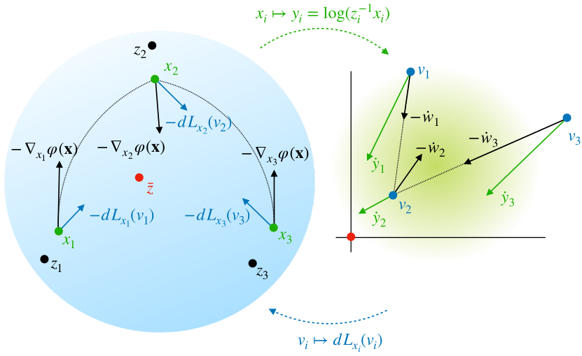
Finally, combining DGF with GT, which is achieved by replacing the term $-\nabla\mathbf{f}({\bm{x}})$ in equation 9 with $-dL_{{\bm{x}}}{\bm{v}}$, gives us Equation 8. In other words, we are “closing the loop” on the DGF by introducing a cost gradient feedback for each agent using GT. A schematic diagram of this design is also depicted in Figure 1(a) with its geometric interpretation in Figure 1(b).

In this section, we run simulations comparing our solver to three other consensus algorithms. We randomly initialized $N=10$ agents ${\bm{x}}\in\mathcal{C}$ and run each algorithm with the same initial conditions in order to compare them. We choose the following two metrics for comparison: the consensus error equation 6, and the rcm Error $\textstyle E_{\mathrm{RCM}}({\bm{x}})=\sum_{i=1}^{N}\mathrm{d}(x_{i},\bar{z})^{2}$ which aggregates the error of each point $x_{1},\ldots,x_{N}$ from the rcm $\bar{z}$. Using these two metrics, we compare our solver against three other algorithms described in the following and illustrate the results in Figure 2. For the technical details of these algorithm and their implementation see the extended version of this work [Kraisler???] and the code [22].

In this scenario, we generate $100$ different problem instances with $N=10$ agents randomly initialized on $\mathcal{C}\subset SO(3)^{10}$. We run the algorithm on each instance for $200$ iterations for visualization of the converge rate. We illustrate the result in Figure 3 showing the statistics of the RCM Error at each time step, confirming a linear rate. We note that although convergences analysis of the algorithm has only been provided for the Euclidean case, these numerical experiments–using different problem parameters–demonstrate the effectiveness of the proposed approach for distributed rcm consensus on Lie groups.

References

- [1] R. Olfati-Saber, J. A. Fax, and R. M. Murray, “Consensus and cooperation in networked multi-agent systems,” Proceedings of the IEEE, vol. 95, no. 1, pp. 215–233, 2007.
- [2] S. H. Strogatz, Sync: How Order Emerges from Chaos in the Universe, Nature, and Daily Life. Hachette UK, 2012.
- [3] S. S. Kia, B. Van Scoy, J. Cortes, R. A. Freeman, K. M. Lynch, and S. Martinez, “Tutorial on dynamic average consensus: The problem, its applications, and the algorithms,” IEEE Control Systems Magazine, vol. 39, no. 3, pp. 40–72, 2019.
- [4] R. Tron, B. Afsari, and R. Vidal, “Riemannian consensus for manifolds with bounded curvature,” IEEE Transactions on Automatic Control, vol. 58, no. 4, pp. 921–934, 2012.
- [5] R. Olfati-Saber, “Swarms on sphere: A programmable swarm with synchronous behaviors like oscillator networks,” in Proceedings of the 45th IEEE Conference on Decision and Control, pp. 5060–5066, IEEE, 2006.
- [6] A. Sarlette, S. Bonnabel, and R. Sepulchre, “Coordinated motion design on Lie groups,” IEEE Transactions on Automatic Control, vol. 55, no. 5, pp. 1047–1058, 2010.
- [7] R. Sepulchre, “Consensus on nonlinear spaces,” IFAC Proceedings Volumes, vol. 43, no. 14, pp. 1029–1039, 2010.
- [8] S. Chen, L. Zhao, W. Zhang, and P. Shi, “Consensus on compact Riemannian manifolds,” Inf. Sci., vol. 268, pp. 220–230, June 2014.
- [9] S. Chen, P. Shi, W. Zhang, and L. Zhao, “Finite-time consensus on strongly convex balls of Riemannian manifolds with switching directed communication topologies,” J. Math. Anal. Appl., vol. 409, pp. 663–675, Jan. 2014.
- [10] S. Kraisler, S. Talebi, and M. Mesbahi, “Distributed consensus on manifolds using the Riemannian center of mass,” IEEE Conference on Control Technology and Applications, 2023.
- [11] R. Tron and R. Vidal, “Distributed 3-d localization of camera sensor networks from 2-d image measurements,” IEEE Transactions on Automatic Control, vol. 59, no. 12, pp. 3325–3340, 2014.
- [12] B. Afsari, “Riemannian center of mass: Existence, uniqueness, and convexity,” Proceedings of the American Mathematical Society, vol. 139, no. 2, pp. 655–673, 2011.
- [13] R. Tron, R. Vidal, and A. Terzis, “Distributed pose averaging in camera networks via consensus on SE(3),” in 2008 Second ACM/IEEE International Conference on Distributed Smart Cameras, pp. 1–10, IEEE, 2008.
- [14] R. Tron, B. Afsari, and R. Vidal, “Average consensus on riemannian manifolds with bounded curvature,” in 2011 50th IEEE Conference on Decision and Control and European Control Conference, pp. 7855–7862, IEEE, 2011.
- [15] J. M. Lee, Introduction to Riemannian Manifolds, vol. 176. Springer, 2nd ed., 2018.
- [16] N. Boumal, An Introduction to Optimization on Smooth Manifolds. Cambridge University Press, 2023.
- [17] A. Arvanitogeōrgos, An Introduction to Lie Groups and the Geometry of Homogeneous Spaces, vol. 22. American Mathematical Soc., 2003.
- [18] Y. L. Sachkov, “Control theory on Lie groups,” Journal of Mathematical Sciences, vol. 156, no. 3, pp. 381–439, 2009.
- [19] J. Milnor, “Curvatures of left invariant metrics on Lie groups,” Advances in mathematics, vol. 21, no. 3, pp. 293–329, 1976.
- [20] A. Nedic, A. Olshevsky, and W. Shi, “Achieving geometric convergence for distributed optimization over time-varying graphs,” SIAM Journal on Optimization, vol. 27, no. 4, pp. 2597–2633, 2017.
- [21] M. Mesbahi and M. Egerstedt, Graph Theoretic Methods in Multiagent Networks. Princeton University Press, 2010.
- [22] S. Kraisler, S. Talebi, and M. Mesbahi, “RCM-Consensus-Lie-Group,” GitHub repository, 2023. Available online at https://github.com/spencerkraisler/RCM-Consensus-Lie-Group.
- [23] A. R. Conn, N. I. Gould, and P. L. Toint, Trust Region Methods. SIAM, 2000.
- [24] D. P. Bertsekas, Constrained Optimization and Lagrange Multiplier Methods. Academic press, 2014.