Abstract

Quantum MASALA: Quantum MAterialS Ab initio eLectronic-structure pAckage

Shri Hari Soundararaj^†‡, Agrim Sharma^† and Manish Jain^$\star$

Centre for Condensed Matter Theory, Department of Physics,

Indian Institute of Science, Bangalore 560012, India

^⋆mjain@iisc.ac.in

August 11, 2026

^$\dagger$^$\dagger$footnotetext: These authors contributed equally to this work^$\ddagger$^$\ddagger$footnotetext: Currently at Materials Science and Engineering, University of California Riverside, Riverside, CA 92521, USA

Abstract

We present Quantum MASALA, a compact package that implements different electronic-structure methods in Python using the plane-wave basis. Within just 8100 lines of pure Python code, we have implemented Density Functional Theory (DFT), Time-dependent Density Functional Theory (TD-DFT) and the GW Method. The program can run across multiple processors and in Graphical Processing Units (GPU) with the help of easily-accessible Python libraries. With Quantum ESPRESSO and BerkeleyGW input interfaces implemented, it can also be used as a substitute for small and medium scale calculations, making it a perfect learning tool for ab initio methods. The package is aimed to provide a framework with its modular and simple code design to rapidly build and test new methods for first-principles calculation.

1 Introduction

Over the last few decades, ab initio electronic structure calculations have become a widespread methodology for studying various properties of molecules and materials. The exponential growth of computation power along with its accessibility has made first-principle calculations ubiquitous in condensed matter studies. Due to its enormous success, density functional theory (DFT)[1, 2] has become the standard technique for computational analysis of both molecular and periodic systems. The GW method[3], although computationally more expensive, has been proven to describe excitations in systems with high accuracy [4].

The development of robust, efficient and massively-parallel computer codes that implement such techniques has massively contributed to their widespread use. DFT Codes like Quantum ESPRESSO[5, 6], ABINIT[7, 8], VASP[9], PARSEC[10] and Octopus[11, 12] have been in active development for decades during which they evolved into feature-rich packages built to be efficient and massively scalable. Similarly, several packages such as BerkeleyGW[4] and YAMBO[13] have a massively parallel implementation of the GW method which has been demonstrated to solve systems containing thousands of atoms.

While being efficient and scalable, the aforementioned packages are not best suited for quickly ‘prototyping’ new ideas and algorithms. During the long development period of these packages, they have evolved into monoliths containing hundreds of thousands of lines of code, resulting in a steep learning curve for newcomers to the package. The general lack of flexibility/customizability in the low-level routines leads to much slower rate of development.

The recent developments in the field of data science have motivated the development of high-throughput screening of materials in order to accelerate the discovery of novel materials and structures[14, 15, 16, 17, 18]. The application of machine learning to electronic structure calculations is also an active field of research. With the rising interests in studying larger and more complex materials in search of novel properties, there is a need to formulate new methods/algorithms that improve the speed and efficiency of ab initio calculations, which is usually the performance bottleneck of such systems.

To address the need for a compact framework, we have designed Quantum MASALA, a Python [19] package aimed to be a suite of electronic structure methods with a simple code design¹¹ 1 Quantum MASALA GitHub repository: https://github.com/qtm-iisc/QuantumMASALA. With less than 8100 lines of pure Python code²² 2 Excluding I/O interfaces with external codes, Quantum MASALA implements the pseudopotential based DFT[20], time-dependent DFT[11, 12] and GW method[21] for periodic solids. Quantum MASALA is designed with minimal required dependencies and supports multiple optional dependencies that enable MPI-parallelism and GPU-Acceleration, maximizing performance in any device. Written in one of the most popular programming languages that is known for its readable syntax, the package aims to provide a sandbox for implementing and testing new ideas quickly.

This article gives a complete description of the Quantum MASALA package. Quantum MASALA is a plane-wave basis based python package which implements different electronic-structure methods. We begin with a brief overview of the theory behind the implemented electronic structure methods which include, the standard plane-wave pseudopotential DFT method, time dependent DFT via a real-time propagation and the GW method. We describe the codebase, starting with a short discussion about runtime performance in Python. We discuss the general layout of the code which includes a brief description of the package’s core modules and structures. The algorithms that are implemented in major calculation routines are described in detail. Finally, we demonstrate the capabilities of the package and provide an analysis of its performance and accuracy in comparison with popular packages. We conclude with a brief summary of the package’s features and future development plans of the code.

2 Theoretical Background

2.1 Density functional theory and the Kohn-Sham equations

Density functional theory relates the ground-state electron density of a given system directly to the total energy. The Kohn-Sham formulation[2] of DFT maps the density of the many-body problem to an independent-particle system that is described by the Kohn-Sham (KS) Hamiltonian (in atomic units):

	$\displaystyle\hat{H}_{\textrm{KS}}\ket{\psi_i}$	$\displaystyle=\bqty{-\frac{1}{2}\laplacian_i + V_{\textrm{aux}}(\mathbf{r}; n(\mathbf{r}))}\ket{\psi_i}$		(1)
	$\displaystyle n(\mathbf{r})$	$\displaystyle=\sum_{i}f_{i}\absolutevalue{\psi_i(\mathbf{r})}^{2}$		(2)

where $f_{i}$ denotes the occupation number of the state $\ket{\psi_i}$ .

The first term of $\hat{H}_{\textrm{KS}}$ is the single-particle kinetic energy operator. The local potential $V_{\textrm{aux}}(\mathbf{r},n(\mathbf{r}))$ depends on the ground-state density $n(\mathbf{r})$ and is given by the following:

V_{\textrm{aux}}(\mathbf{r};n(\mathbf{r}))=V_{\textrm{ext}}(\mathbf{r})+V_{\textrm{Hartree}}(\mathbf{r};n(\mathbf{r}))+V_{\textrm{xc}}(\mathbf{r};n(\mathbf{r}))

(3)

where $V_{ext}$ is the external potential, which in the case of the electronic structure problems is the Coulomb potential generated by the nuclei. The Hartree potential is the classical potential on an electron due to charge density and the exchange-correlation (XC) potentials represents the remaining many-body interaction. Note that $V_{\textrm{xc}}$ can be spin-dependent based on the choice of the XC functional.

The density dependence of the potential in $\hat{H}_{\textrm{KS}}$ requires the ground-state solution to be self-consistent with the potential in the Hamiltonian. Therefore, solving the KS system requires an self-consistent-field (SCF) iteration, which involves the following sequence of quantities to be evaluated:

$\displaystyle n_{1}\rightarrow V_{1}\rightarrow\quantity{\ket{\psi_i}}_{1}\rightarrow$	$\displaystyle n_{\textrm{out},1}\xRightarrow[\text{mix}]{n_{\textrm{out},1}\neq n_{1}}n_{2}$	(4)
$\displaystyle n_{2}\rightarrow V_{2}\rightarrow\quantity{\ket{\psi_i}}_{2}\rightarrow$	$\displaystyle n_{\textrm{out},2}\xRightarrow[\text{mix}]{n_{\textrm{out},2}\neq n_{2}}n_{3}$	(5)
		(6)
$\displaystyle n_{N}\rightarrow V_{N}\rightarrow\quantity{\ket{\psi_i}}_{N}\rightarrow$	$\displaystyle n_{\textrm{out},N}\xRightarrow{n_{\textrm{out},N}=n_{N}}n_{N}\equiv n_{\textrm{KS}}$	(7)

The number of steps required for achieving self-consistency can be reduced using fixed-point iteration algorithms, which involves a mixing of densities of input, output, and in some methods, values from previous iterations too.

2.2 Wavefunctions in Periodic Solids and the Plane-Wave Basis

In periodic solids, according to Bloch’s Theorem, the wavefunctions of the KS Hamiltonian can be written as:

\ket{\psi_i}\rightarrow\ket{\psi_{\mathbf{k}}^i};\innerproduct{\mathbf{r}}{\psi_{\mathbf{k}}^i}={}_{\mathbf{k}}^{i}(\mathbf{r}):=e^{i\mathbf{k}\cdot\mathbf{r}}u_{\mathbf{k}}^{i}(\mathbf{r})

(8)

where $u_{\mathbf{k}}^{i}(\mathbf{r})$ has the periodicity of the crystal. The periodic function $u_{\mathbf{k}}^{i}(\mathbf{r})$ can be expressed as a Fourier series, using the plane wave expansion

	$\displaystyle\innerproduct{\mathbf{r}}{\psi_{\mathbf{k}}^i}$	$\displaystyle=e^{i\mathbf{k}\cdot\mathbf{r}}\cdot\sum_{\mathbf{G}}u_{\mathbf{k}}^{i}(\mathbf{G})e^{i\mathbf{G}\cdot\mathbf{r}}$		(9)
		$\displaystyle=\sum_{\mathbf{G}}u_{\mathbf{k}}^{i}(\mathbf{G})\innerproduct{\mathbf{r}}{\mathbf{G}+\mathbf{k}};\innerproduct{\mathbf{r}}{\mathbf{G} + \mathbf{k}}:=e^{i(\mathbf{G}+\mathbf{k})\cdot\mathbf{r}}$		(10)

where $\mathbf{G}$ are the lattice points of the reciprocal lattice of the crystal.

The KS Hamiltonian in the plane wave (PW) basis takes the following form:

	$\displaystyle\matrixelement{\mathbf{G}_m + \mathbf{k}}{\hat{H}_{\textrm{KS}}}{\mathbf{G}_n+\mathbf{k}}$	$\displaystyle=\matrixelement{\mathbf{G}_{m + \mathbf{k}}}{\bqty{-\frac{1}{2}\laplacian+ V_{\textrm{KS}}(\mathbf{r})}}{\mathbf{G}_n + \mathbf{k}}$		(11)
	$\displaystyle H_{m,n}(\mathbf{k})$	$\displaystyle=\frac{\absolutevalue{\mathbf{k} + \mathbf{G}_m}^{2}}{2}\delta_{m,n}+V_{\textrm{KS}}(\mathbf{G}_{m}-\mathbf{G}_{n})$		(12)

For solving the system numerically, the PW basis is truncated. The wave functions are expanded including only those plane waves whose energy is less than a energy cutoff, $E_{\textrm{cut}}$ i.e. ( $\absolutevalue{\mathbf{k} + \mathbf{G}_m}^{2}/2\leq E_{\textrm{cut}}$ ). This implies that the PW expansion of $V_{\textrm{KS}}$ must contain $G$ within the energy cutoff $4E_{\textrm{cut}}$ as $\absolutevalue{\mathbf{G}_m - \mathbf{G}_n}\leq\absolutevalue{\mathbf{G}_m}+\absolutevalue{\mathbf{G}_n}\leq 2\sqrt{2E_{\textrm{cut}}}$

2.3 Pseudopotentials

Most chemical behaviour of atoms originate from the behaviour of the valence electrons which is influenced by their surrounding chemical environment. The core electrons, which remain unaffected under most situations, can be replaced with an effective ‘pseudo-potential’ on the valence electrons that can accurately reproduce their states across a wide range of conditions. As pseudopotentials aim to replace the potential generated by the nucleus and core electrons, they must be spherically symmetric where each $(l,m)$ is treated individually. The ‘semi-local’ form of a pseudopotential of an atom centred at origin is given below:

\hat{V}_{ps}=\sum_{l}\sum_{m=-l}^{l}\ket{l,m}V^{l}(r)\bra{l,m}

(13)

This form can be simplified to a sum of projection operators, as given by Kleinman and Bylander[22]:

\hat{V}_{ps}=V_{loc}(\mathbf{r})+\sum_{(l,m)}\frac{\outerproduct{\Delta V_{ps}^l \varphi_{lm}}{\Delta V_{ps}^l \varphi_{lm}}}{\expectationvalue{\Delta V_{ps}^l}{\varphi_{lm}}};\;\Delta V_{ps}^{l}=V^{l}-V_{loc}

(14)

2.4 Time-dependent Density Functional Theory

The Time-Dependent Density Functional Theory[23] extends DFT from describing ground-state properties to evaluating the real-time dynamics, enabling it to compute excited state properties and response to time-dependent perturbations. The time-dependent Kohn-Sham (TDKS) equations take a form that is analogous to the time-dependent Schrodinger equation:

$\displaystyle i\partialderivative{t}\ket{\psi_i}$	$\displaystyle=\hat{H}_{\textrm{KS}}(t)\ket{\psi_i}$	(15)
	$\displaystyle=\bqty{-\frac{1}{2}\laplacian+ V_{\textrm{KS}}(\mathbf{r}, t; n(\mathbf{r}, t))}\ket{\psi_i}$	(16)
$\displaystyle n(\mathbf{r},t)$	$\displaystyle=\sum_{i}f_{i}\absolutevalue{\psi_i(\mathbf{r},t)}^{2}$	(17)

The potential term $V_{\textrm{KS}}(\mathbf{r},t)$ here is analogous to the time-independent equations, containing a time-varying external potential $V_{ext}(\mathbf{r},t)$ . For the XC Potentials in TDDFT, we limit ourselves to adiabatic approximations where $V_{\textrm{xc}}(\mathbf{r},t;n(\mathbf{r},t)):=V_{\textrm{xc}}(\mathbf{r};n(\mathbf{r},t))$

The formal solution of the TDKS Equations is given by:

	$\displaystyle\ket{\psi_i(t)}$	$\displaystyle=\mathcal{T}\exp{-i \int_0^t \dd{\tau} \hat{H}_{\textrm{KS}}(\tau)}\ket{\psi_i(t=0)}$		(18)
		$\displaystyle=\hat{U}_{\textrm{KS}}(t,0)\ket{\psi_i(t=0)}$		(19)

where $\mathcal{T}$ denotes the time-ordering operator. The time-evolution operator $\hat{U}(t^{\prime},t)$ can be split into smaller time-steps:

\hat{U}(t_{N},t_{0})=\hat{U}(t_{N},t_{N-1})\cdot\hat{U}(t_{N-1},t_{N-2})\cdots\hat{U}(t_{2},t_{1})\cdot\hat{U}(t_{1},t_{0});\;t_{n}=t_{0}+n\Delta t

(20)

TDDFT can be used to compute the optical absorption spectra by propagating the TDKS equations. By perturbing the ground-state system with a delta electric field along, lets say x-axis, $v_{pert}(\mathbf{r},t)=-k_{0}\delta(t)\cdot(\mathbf{r}\cdot\hat{x})$ , the system evolves in time with a density response $\delta n(\mathbf{r},t)=n(\mathbf{r},t)-n_{0}(\mathbf{r})$ . For small perturbation $k_{0}<<1$ , the response is expected to be linear and dipolar, allowing us to compute the dynamical polarizability from the dipole response

\alpha_{x\nu}(\omega)=-\frac{1}{k_{0}}\int\differential[]r\delta n(\mathbf{r},\omega)r_{\nu};\;\ \nu=x,y,z

(21)

The absorption cross-section is proportional to the imaginary part of $\alpha$ averaged over the three spatial directions.

\sigma(\omega)=\frac{4\pi\omega}{c}\cdot\mathfrak{Im}\frac{1}{3}\sum_{\nu}\alpha_{\nu\nu}(\omega)

(22)

2.5 GW Approximation

Kohn-Sham DFT yields the correct ground state electron density, but the corresponding non-interacting single-particle orbitals need not have any direct physical interpretation[3, 24, 25]. Electron addition and removal energies are quasiparticle energies and its calculation requires many-body effects to be taken into account[3, 21, 26]. This can be done using Hedin’s GW formalism [3], where one directly calculates the quasiparticle energies as poles of the single particle Green’s function. Within this formalism, the exact many-body self-energy is expressed as a perturbation series in terms of dynamically screened Coulomb interaction.

While in principle, to calculate the poles of the single-particle Greens function one needs to solve the Dyson equation, often, the quasiparticle energies are computed as a single shot correction to the DFT energy eigenvalues. Within this approach the Greens function ( $\textrm{G}_{0}$ ) and screened Coulomb interaction ( $\textrm{W}_{0}$ ) are constructed from DFT orbitals and energy eigenvalues. For a large variety of materials, the first iteration is good enough for calculating the quasiparticle energy spectrum[27]. This method of doing a single GW iteration is known as the G₀W₀ method.

Written explicitly, we are interested in solving

\left[-\frac{1}{2}\hat{\nabla}^{2}+\hat{V}_{\textrm{ext}}+\hat{V}_{\textrm{Hartree}}+\hat{\Sigma}(E_{n\bf k})\right]\,{}_{n\bf k}^{\text{QP}}=E_{n\bf k}\,{}_{n\bf k}^{\text{QP}}

(23)

where $\hat{\Sigma}$ is the G₀W₀ dynamical self energy operator which is non-local, and non-Hermitian in general[21]. As a result, the quasiparticle energy eigenvalues $E_{n\bf k}$ are complex - their imaginary parts being inversely related to quasiparticle lifetimes. While calculating the quasiparticle energy spectrum, $E_{n\textbf{k}}^{\textrm{QP}}=\textrm{Re}\left(E_{n\textbf{k}}\right)$ for quasiparticles with long lifetimes, it is common practice to solve the real part of eqn. 23, while evaluating the self energy operator $\hat{\Sigma}(E)$ at $E_{n\textbf{k}}^{\textrm{QP}}$ , instead of $E_{n\textbf{k}}$ . Further, in a typical calculation, the DFT eigenvectors are sufficiently close to the quasiparticle eigenvectors [4] for the following approximation to be used:

E_{n\bf k}^{\text{QP}}=E_{n\bf k}^{\text{DFT}}+\bra{\psi_{n\bf k}^{\text{DFT}}}\left(\hat{\Sigma}\left(E_{n\bf k}^{\textrm{QP}}\right)-V_{\textrm{xc}}\right)\ket{\psi_{n\bf k}^{\text{DFT}}}

(24)

The $G_{0}W_{0}$ self-energy $\Sigma$ is defined as[3]:

\Sigma\left(\textbf{r},\textbf{r}^{\prime};t,t^{\prime}\right)=i\,G_{0}\left(\textbf{r},\textbf{r}^{\prime};t,t^{\prime}\right)\,W_{0}\left(\textbf{r},\textbf{r}^{\prime};t\!+\!0^{+},t^{\prime}\right)

(25)

where $G_{0}(\textbf{r},\textbf{r}^{\prime};t,t^{\prime})$ is the single particle Green’s function

G_{0}\left(\textbf{r},\textbf{r}^{\prime};t,t^{\prime}\right)=-i\bra{N}T\left[\hat{\psi}^{\dagger}\left(\textbf{r}^{\prime},t^{\prime}\right)\,\hat{\psi}\left(\textbf{r},t\right)\right]\ket{N}

(26)

and $W_{0}(\textbf{r},\textbf{r}^{\prime};t,t^{\prime})$ is screened Coulomb interaction

W_{0}\left(\textbf{r},\textbf{r}^{\prime};t,t^{\prime}\right)=\int\epsilon^{-1}\left(\textbf{r},\textbf{r}^{\prime\prime};t,t^{\prime}\right)\,v\left(\textbf{r}^{\prime\prime},\textbf{r}^{\prime}\right)\,\textrm{d}\textbf{r}^{\prime\prime}

(27)

In time translation invariant systems, the self energy effectively becomes a function of $t-t^{\prime}$ instead of $t$ and $t^{\prime}$ . The same holds for $G_{0}$ , $W_{0}$ , and $\epsilon$ .

In the rest of the section we will use Rydberg units. In the plane wave basis, the random phase approximation (RPA) dielectric function is:

\epsilon_{\textbf{GG'}}{\left({\textbf{q}}\;\!;\omega\right)}=\delta_{\textbf{GG'}}\,{-}\,v{\left({\textbf{q}}{+}{\textbf{G}}\right)}\,P_{\textbf{GG'}}{\left({\textbf{q}}\;\!;\omega\right)}

(28)

where G and $\textbf{G}^{\prime}$ are reciprocal lattice vectors, q lies in the first Brillouin zone, $v(\textbf{q}+\textbf{G})$ is bare Coulomb potential:

v(\textbf{q}+\textbf{G})=\frac{8\pi}{\left|\textbf{q}+\textbf{G}\right|^{2}}

(29)

and $P$ is irreducible polarizability, for which the Adler-Wiser expression simplifies to[4]:

P_{\textbf{GG'}}{\left({\textbf{q}}\;\!;\omega=0\right)}=\,\,{}\sum_{n}^{\textrm{occ}}\sum_{n^{\prime}}^{\textrm{emp}}\sum_{{\textbf{k}}}\frac{\bra{n'\textbf k}e^{-i({\textbf{q}}+{\textbf{G}})\cdot{\textbf{r}}}\ket{n{\textbf k}{+}{\textbf q}}\bra{n{\textbf k}{+}{\textbf q}}e^{i({\textbf{q}}+{\textbf{G}^{\prime}})\cdot{\textbf{r}}}\ket{n'\textbf k}}{E_{n{\textbf{k}}{+}{\textbf{q}}}\,{-}\,E_{n^{\prime}{\textbf{k}}}}.

(30)

In the GW formalism, the real part of self-energy as defined above naturally splits into two parts: the product of the real parts of $G_{0}$ and $W_{0}$ gives the screened exchange (SX) term and the product of their imaginary parts gives the Coulomb-hole (CH) term. [28]

\real\left(\Sigma\right)=\Sigma_{\textrm{SX}}+\Sigma_{\textrm{CH}}

(31)

Under the static COHSEX approximation proposed by Hedin[3], the self-energy matrices can be expressed as:

	$\displaystyle\left<n{\textbf{k}}\right\|\Sigma_{\textrm{SX}}{\left(E=0\right)}\left\|n^{\prime}{\textbf{k}}\right>=-\sum_{n^{\prime\prime}}^{\textrm{occ}}\sum_{\textbf{qGG'}}$	$\displaystyle\left<n{\textbf{k}}\right\|e^{i({\textbf{q}}+{\textbf{G}})\cdot{\textbf{r}}}\left\|n^{\prime\prime}{\textbf{k}}{-}{\textbf{q}}\right>\left<n^{\prime\prime}{\textbf{k}}{-}{\textbf{q}}\right\|e^{-i({\textbf{q}}+{\textbf{G}}^{\prime})\cdot{\textbf{r}}^{\prime}}\left\|n^{\prime}{\textbf{k}}\right>$
		$\displaystyle\text{ }\;\;\times\epsilon_{\textbf{GG'}}^{-1}{\left({\textbf{q}}\;\!;0\right)}v{\left({\textbf{q}}{+}{\textbf{G}}^{\prime}\right)}$		(32)

$\displaystyle\left<n{\textbf{k}}\right\|\Sigma_{\textrm{CH}}{\left(E=0\right)}\left\|n^{\prime}{\textbf{k}}\right>$	$\displaystyle=\frac{1}{2}\sum_{n^{\prime\prime}}\sum_{\textbf{qGG'}}\left<n{\textbf{k}}\right\|e^{i({\textbf{q}}+{\textbf{G}})\cdot{\textbf{r}}}\left\|n^{\prime\prime}{\textbf{k}}{-}{\textbf{q}}\right>\left<n^{\prime\prime}{\textbf{k}}{-}{\textbf{q}}\right\|e^{-i({\textbf{q}}+{\textbf{G}}^{\prime})\cdot{\textbf{r}}^{\prime}}\left\|n^{\prime}{\textbf{k}}\right>$
	$\displaystyle\text{\hskip 60.00009pt}\times\left[\epsilon_{\textbf{GG'}}^{-1}{\left({\textbf{q}}\;\!;0\right)}\,{-}\,\delta_{\textbf{GG'}}\right]v{\left({\textbf{q}}{+}{\textbf{G}}^{\prime}\right)}$	(33)
	$\displaystyle=\frac{1}{2}\sum_{\textbf{qGG'}}\left<n{\textbf{k}}\right\|e^{i({\textbf{G}}-{\textbf{G}}^{\prime})\cdot{\textbf{r}}}\left\|n^{\prime}{\textbf{k}}\right>\left[\epsilon_{\textbf{GG'}}^{-1}{\left({\textbf{q}}\;\!;0\right)}\,{-}\,\delta_{\textbf{GG'}}\right]v{\left({\textbf{q}}{+}{\textbf{G}}^{\prime}\right)}$	(34)

We note that the completeness relation of mutually orthogonal orbitals has been used in (eq.34), to skip the expensive summation over all bands. Also note that conventionally, the self energy is expanded as the sum of a Hartree-Fock exchange term and a (Coulomb) correlation term:

\Sigma=\Sigma_{\textrm{X}}+\Sigma_{\textrm{Corr}}

(35)

The Hartree-Fock exchange matrix elements can be calculated as follows:

	$\displaystyle\left<n{\textbf{k}}\right\|\Sigma_{\textrm{X}}\left\|n^{\prime}{\textbf{k}}\right>=-\sum_{n^{\prime\prime}}^{\textrm{occ}}\sum_{\textbf{qGG'}}$	$\displaystyle\left<n{\textbf{k}}\right\|e^{i({\textbf{q}}+{\textbf{G}})\cdot{\textbf{r}}}\left\|n^{\prime\prime}{\textbf{k}}{-}{\textbf{q}}\right>\left<n^{\prime\prime}{\textbf{k}}{-}{\textbf{q}}\right\|e^{-i({\textbf{q}}+{\textbf{G}}^{\prime})\cdot{\textbf{r}}^{\prime}}\left\|n^{\prime}{\textbf{k}}\right>$
		$\displaystyle\text{ }\;\;\times\delta_{\textbf{GG'}}v{\left({\textbf{q}}{+}\textbf{G'}\right)}$		(36)

The correlation term captures the effect of screening due to other electrons. We can identify the real part of the correlation term to be $\textrm{Re}\left(\Sigma_{\textrm{Corr}}\right)=\left(\Sigma_{\textrm{SX}}-\Sigma_{\textrm{X}}\right)+\Sigma_{\textrm{CH}}$ .

Beyond Static-COHSEX, dynamical self-energy needs to be solved self-consistently, as shown below.

	$\displaystyle E_{n\textbf{k}}^{\textrm{QP}}$	$\displaystyle=\textrm{Re}\left(E_{n\textbf{k}}\right)$		(37)
		$\displaystyle=\textrm{Re}\left(\Sigma_{n\textbf{k}}\left(E_{n\textbf{k}}^{\textrm{QP}}\right)\right)+E_{n\bf k}^{\text{DFT}}-V_{\textrm{xc},n\bf k}^{\text{DFT}}$		(38)

The Hybertsen-Louie plasmon pole model [21] assumes that contribution from a single plasmon dominates the pole structure of the inverse dielectric function. Using Kramers-Kronig relations and a generalized f-sum rule [21], one can get rid of all free parameters in the single plasmon dielectric function [28], and the static dielectric function value can be used to generate values at all frequencies. With this approximation, we obtain the following self-energy matrix elements:

	$\displaystyle\left<n{\bf k}\right\|\Sigma_{\textrm{SX}}{\left(E\right)}\left\|n^{\prime}{\bf k}\right>=-\sum_{n^{\prime\prime}}^{\textrm{occ}}\sum_{{\bf qGG}^{\prime}}\left<n{\bf k}\right\|e^{i({\bf q}+{\bf G})\cdot{\bf r}}\left\|n^{\prime\prime}{\bf k}{-}{\bf q}\right>\left<n^{\prime\prime}{\bf k}{-}{\bf q}\right\|e^{-i({\bf q}+{\bf G}^{\prime})\cdot{\bf r}^{\prime}}\left\|n^{\prime}{\bf k}\right>$		(39)
	$\displaystyle\times\left[\delta_{{\bf GG}^{\prime}}+\frac{{}^{2}_{{\bf GG}^{\prime}}{\left({\bf q}\;\!\right)}\left(1\,{-}\,i\tan\phi_{{\bf GG}^{\prime}}{\left({\bf q}\;\!\right)}\right)}{\left(E\,{-}\,E_{n^{\prime\prime}{\bf k}{-}{\bf q}}\right)^{2}\!{-}\>\tilde{\omega}^{2}_{{\bf GG}^{\prime}}{\left({\bf q}\;\!\right)}}\right]v{\left({\bf q}{+}{\bf G}^{\prime}\right)}$

	$\displaystyle\left<n{\bf k}\right\|\Sigma_{\textrm{CH}}{\left(E\right)}\left\|n^{\prime}{\bf k}\right>=\frac{1}{2}\sum_{n^{\prime\prime}}\sum_{{\bf qGG}^{\prime}}\left<n{\bf k}\right\|e^{i({\bf q}+{\bf G})\cdot{\bf r}}\left\|n^{\prime\prime}{\bf k}{-}{\bf q}\right>\left<n^{\prime\prime}{\bf k}{-}{\bf q}\right\|e^{-i({\bf q}+{\bf G}^{\prime})\cdot{\bf r}^{\prime}}\left\|n^{\prime}{\bf k}\right>$		(40)
	$\displaystyle\times\,\frac{{}^{2}_{{\bf GG}^{\prime}}{\left({\bf q}\;\!\right)}\left(1\,{-}\,i\tan\phi_{{\bf GG}^{\prime}}{\left({\bf q}\;\!\right)}\right)}{\tilde{\omega}_{{\bf GG}^{\prime}}{\left({\bf q}\;\!\right)}\left(E\,{-}\,E_{n^{\prime\prime}{\bf k}{-}{\bf q}}{-}\,\tilde{\omega}_{{\bf GG}^{\prime}}{\left({\bf q}\;\!\right)}\right)}\;v{\left({\bf q}{+}{\bf G}^{\prime}\right)}$

where the plasmon mode parameters are defined as follows:
The effective bare plasma frequency:

{}^{2}_{{\bf GG}^{\prime}}{\left({\bf q}\;\!\right)}=\omega_{\textrm{p}}^{2}\,\,\frac{{\left({\bf q}{+}{\bf G}\right)}{\cdot}{\left({\bf q}{+}{\bf G}^{\prime}\right)}}{\left|{\bf q}{+}{\bf G}\right|^{2}}\,\,\frac{\rho{\left({\bf G}{-}{\bf G}^{\prime}\right)}}{\rho{\left({\bf 0}\right)}}

(41)

the GPP mode frequency:

\tilde{\omega}^{2}_{{\bf GG}^{\prime}}{\left({\bf q}\;\!\right)}=\frac{\left|\lambda_{{\bf GG}^{\prime}}{\left({\bf q}\;\!\right)}\right|}{\cos\phi_{{\bf GG}^{\prime}}{\left({\bf q}\;\!\right)}}

(42)

and the renormalized bare plasmon frequency:

\left|\lambda_{{\bf GG}^{\prime}}{\left({\bf q}\;\!\right)}\right|e^{i\phi_{{\bf GG}^{\prime}}{\left({\bf q}\;\!\right)}}=\frac{{}^{2}_{{\bf GG}^{\prime}}{\left({\bf q}\;\!\right)}}{\delta_{{\bf G}{\bf G}^{\prime}}{-}\epsilon_{{\bf G}{\bf G}^{\prime}}^{-1}({\bf q};0)}

(43)

where, $\rho$ denotes the electron charge density and $\omega_{\textrm{p}}^{2}=4\pi\rho({\bf 0})e^{2}/m$ denotes the classical plasma frequency.

Divergent cases arising from the above equations are handled as per the prescription given in BerkeleyGW[4]. Due to the $n^{\prime\prime}$ -dependence of $\epsilon_{\textrm{HLPP}}$ , it is not possible to get rid of the $n^{\prime\prime}$ summation over all orbitals in $\Sigma_{\textrm{CH}}$ calculation. However, several methods have been devised to reduce the number of empty orbitals required to make this sum converge. Static remainder approach discussed in [29] is one such scheme,

	$\displaystyle\left<n{\bf k}\right\|\Sigma_{\textrm{CH}}^{\infty}{\left(E\right)}\left\|n^{\prime}{\bf k}\right>=$	$\displaystyle\left<n{\bf k}\right\|\Sigma_{\textrm{CH}}^{N}{\left(E\right)}\left\|n^{\prime}{\bf k}\right>$		(44)
		$\displaystyle+\frac{1}{2}\bigg(\left<n{\bf k}\right\|\Sigma_{\textrm{CH}}^{\infty}{\left(E=0\right)}\left\|n^{\prime}{\bf k}\right>-\left<n{\bf k}\right\|\Sigma_{\textrm{CH}}^{N}{\left(E=0\right)}\left\|n^{\prime}{\bf k}\right>\bigg)$

where $N$ or $\infty$ denote the number of empty orbitals included in $n^{\prime\prime}$ summation and ‘ $E=0$ ’ denotes static-COHSEX self-energies.

Dynamic self-energy calculated with plasmon-pole method depend on energy parameter $E$ . In order to avoid a series of self-consistent iterations to compute $E_{n\textbf{k}}^{\textrm{QP}}$ , we compute $\Sigma_{\textrm{HLPP}}$ for two different sets of energies and then find $E_{n\textbf{k}}^{\textrm{QP}}$ using the secant method:

E^{\textrm{QP}}_{n{\bf k}}=E^{0}_{n{\bf k}}+\frac{d\Sigma/dE}{1-d\Sigma/dE}\left(E^{0}_{n{\bf k}}-E^{\textrm{MF}}_{n{\bf k}}\right)

(45)

where $E^{0}_{n{\bf k}}=\Sigma_{\textrm{HLPP}}\big(E^{\textrm{MF}}_{n{\bf k}}\big)$ and $d\Sigma/dE$ is calculated using a forward finite difference scheme.

3 Writing performant code in Python: Libraries used

Python, as a programming language, is considered to be slow in comparison to compiled languages like C, C++, FORTRAN, etc. The reference implementation, CPython[19], is not as fast as other interpreted languages like MATLAB, Julia, R, etc. due to a lack of optimizations in its bytecode interpreter. High-throughput in Python is usually achieved by libraries and packages that have their core implementations written in ‘faster’ languages, usually C. The data structures and routines implemented can be accessed from Python via defined interfaces. For a Python program to be ‘efficient’ in comparison to its analogues written in a compiled program, it is important to maximize the amount of processing that can be performed in each call to optimised routines implemented in these libraries.

There are alternative strategies for speeding up Python. Some of the relevant ones are listed below:

•

PyPy[30] is an alternative implementation of Python that implements Just-In-Time (JIT) Compilation to speed up execution.
•

Numba[31] is a third-party package that brings JIT Compilation to CPython.
•

Cython[32] extends Python with C-like syntax and compilation support that results in performance similar to a C/C++ code.

We have refrained from using the aforementioned optimization tools in order to maximize compatibility and reduce dependencies, but we encourage developers to try them when extending our package for their needs wherever applicable.

Quantum MASALA uses NumPy[33] for performing all linear algebra operations. The library provides support for multi-dimensional array of homogeneous data along with an extensive set of routines implementing mathematical operations and linear algebra algorithms. It is easy-to-use and interoperable across most scientific computing packages in Python. The library calls optimized BLAS and LAPACK functions for linear algebra operations, allowing access to near C/FORTRAN speeds in Python.

Analogous to NumPy, CuPy[34] is a Python library that contains implementations of a subset of NumPy operations to run in an NVIDIA GPU. It provides a NumPy-like interface to Arrays in GPU Memory with nearly identical function calls to operate on them. This enables Quantum MASALA to run computationally intensive part of a calculation like FFT’s, diagonalization, etc. in a GPU. As a part of its design, Quantum MASALA reuses a lot of the CPU code for its GPU implementation, which is possible due to NumPy’s interoperability with CuPy.

Quantum MASALA can also use FFT Libraries like FFTW3 (via pyFFTW[35]) and MKL (via mkl_fft[36]) if already installed. If not installed, the program automatically falls back to the slower FFT routines implemented in SciPy[37].

4 Usage: Core Objects of Quantum MASALA

4.1 Installation

The code for Quantum MASALA is available as a git repository at https://github.com/qtm-iisc/QuantumMASALA. The code supports Python version 3.9 and beyond.

These installation instructions require conda. If you do not have a functioning conda installation, we recommend installing it by following these quick-install instructions: https://docs.conda.io/projects/miniconda/en/latest/#quick-command-line-install

4.1.1 Installing on Mac

To create the necessary environment, execute the following command:

⬇

pyfftw pylibxc mpi4py scipy cython

Note: For older versions of Python, it may be necessary to install numpy separately with Apple’s Accelerate framework. With newer versions of numpy (> 2.0), the wheels are automatically built with Apple’s Accelerate framework (Veclib).

Activate the environment:

To test the numpy and scipy installation, install the following packages:

⬇

pooch pyyaml

Note: Please verify that the python command points to the environment’s Python installation by running which python. If it does not point to the correct Python installation, we recommend specifying the full python path (i.e., $CONDA_PREFIX/bin/python) for the following commands.

To test numpy and scipy, use the following commands:

⬇

import numpy

numpy.show_config()

numpy.test()

import scipy

scipy.show_config()

scipy.test()

For optimal performance, we recommend setting the relevant ..._NUM_THREADS environment variables to 1:

⬇

conda env config vars set VECLIB_MAXIMUM_THREADS=1

conda env config vars set OPENBLAS_NUM_THREADS=1

Reactivate the environment for the changes to take effect:

⬇

conda activate qtm

Inside the QuantumMASALA root directory, execute the following command to complete the installation:

Test the installation by running the following example (replace 2 with the number of cores):

⬇

mpirun -np 2 python si_scf.py

To perform a complete test, use pytest from the main directory which contains the tests folder:

⬇

pytest

4.1.2 Installing on Linux

To create the environment, execute the following commands:

⬇

conda activate qtm

conda install -c conda-forge pyfftw pylibxc mpi4py

If you are working on an Intel system, we recommend using mkl_fft for optimal performance:

For optimal performance, we recommend setting the OMP_NUM_THREADS environment variable to 1:

Reactivate the environment for the changes to take effect:

⬇

conda activate qtm

Inside the QuantumMASALA root directory, execute the following command to complete the installation:

Test the installation by running the following example (replace 2 with the number of cores):

⬇

mpirun -np 2 python si_scf.py

To perform a complete test, use pytest from the main directory which contains the tests folder:

⬇

pytest

4.1.3 Optional Dependencies

The user may choose to install with optional libraries for added features. GPU support is provided by CuPy[34]. The instructions for installing CuPy are available at: https://docs.cupy.dev/en/stable/install.html. If a CUDA driver is already installed, the following command can be used to install both CUDA-Toolkit and CuPy from conda-forge:

The Python package primme provides interface to PRIMME[38], a C library for iterative solution of eigenvalue problems.

4.1.4 Compiling the Documentation

We use Sphinx to compile documentation from the docstrings. The documentation is available on ’Read the Docs’ at https://quantummasala.readthedocs.io/en/latest/, and can also be compiled locally.

To compile the documentation locally using Sphinx, install the following packages:

Compile the reStructuredText documentation by running the following from the root directory:

Build the documentation in HTML format by running the following from the root directory:

4.2 Defining a Crystal in Quantum MASALA

In Quantum MASALA, the lattice of translations is represented by the Lattice class. This class contains the primitive translation vectors and provides methods for coordinate transformation. The RealLattice and the ReciLattice classes extend the Lattice class with lattice parameter ‘ $a$ ’ which is alat for RealLattice and tpiba ( $2\pi/a$ ) for ReciLattice. The two subclasses also provide methods to instantiate from instances of their duals. Some usage examples are highlighted below:

⬇

from qtm.lattice import RealLattice, ReciLattice

from qtm.constants import ANGSTROM

# Defining a BCC Lattice

alat = 5.1 * ANGSTROM # Lattice parameter ’a’

# Lattice vectors

latvec_alat = 0.5 * np.array([

[ 1, 1, 1],

[-1, 1, 1],

[-1, -1, 1]

])

# Creating RealLattice instance representing BCC lattice

reallat = RealLattice.from_alat(alat, *latvec_alat)

# Creating ReciLattice instance from reallat

recilat = ReciLattice.from_reallat(reallat)

# Printing axes

print(reallat.alat, reallat.axes_alat)

## 9.637603235591428 ([0.5, 0.5, 0.5], [-0.5, 0.5, 0.5], [-0.5, -0.5, 0.5])

print(recilat.tpiba, recilat.axes_tpiba)

## 0.6519447993019614 ([1.0, 0.0, 1.0], [-1.0, 1.0, 0.0], [0.0, -1.0, 1.0])

# Input array of vectors in crystal coordinates

vec_cryst = np.array([

[1, 0, 0],

[0, 1, 0],

[1, 1, 0],

[0, 1, 1]

])

# Coordinate Transforms

vec_cart = reallat.cryst2cart(vec_cryst, axis=1)

print(vec_cart)

## [[ 4.81880162 4.81880162 4.81880162]

## [-4.81880162 4.81880162 4.81880162]

## [ 0. 9.63760324 9.63760324]

## [-9.63760324 0. 9.63760324]]

vec_alat = reallat.cryst2alat(vec_cryst, axis=1)

print(vec_alat)

## [[ 0.5 0.5 0.5]

## [-0.5 0.5 0.5]

## [ 0. 1. 1. ]

## [-1. 0. 1. ]]

# NOTE: As per convention, the first dimension of vector lists

# must correspond to the components, resulting in a shape of

# form (3, …)

len_alat = reallat.norm(vec_cryst.T, coords=’cryst’)

print(len_alat / reallat.alat)

## [0.8660254 0.8660254 1.41421356 1.41421356]

A crystal can be fully specified by the lattice and the atoms in the unit cell. Similarly, the Crystal class in Quantum MASALA is defined by:

1.

A RealLattice instance describing the lattice of the crystal
2.

A sequence of AtomBasis instances describing the crystal’s basis atoms

The AtomBasis class represent a collection of atoms in the unit cell belonging to one atomic species/type and describes the position of the atoms in the crystal’s unit cell along with the species’ name, mass, and optionally its pseudopotential. Note that for DFT calculations, the pseudopotential is a required argument. Currently Quantum MASALA supports the UPF v2 format only via the UPFv2Data container.

⬇

from qtm.lattice import RealLattice

from qtm.crystal import BasisAtoms, Crystal

from qtm.pseudo import UPFv2Data

from qtm.constants import BOHR

# Defining the lattice

reallat = RealLattice.from_alat(alat=5.1070 * BOHR,

a1=[ 0.5, 0.5, 0.5],

a2=[-0.5, 0.5, 0.5],

a3=[-0.5, -0.5, 0.5])

# Reading pseudopotential data

fe_oncv = UPFv2Data.from_file(’../examples/dft-fe/Fe_ONCV_PBE-1.2.upf’)

# Specifying the basis atoms

fe_atoms = BasisAtoms.from_cart(’fe’, fe_oncv, 55.487, reallat,#

[0.0, 0.0, 0.0])

# Constructing the Crystal instance

crystal = Crystal(reallat, [fe_atoms, ])

# Printing crystal information

print(str(crystal))

Output

Lattice parameter ’alat’ : 5.10700  a.u.
Unit cell volume         : 66.59898  (a.u.)ˆ3
Number of atoms/cell     : 1
Number of atomic types   : 1
Number of electrons      : 16

Crystal Axes: coordinates in units of ’alat’ (5.10700 a.u.)
    a(1) = ( 0.50000,  0.50000,  0.50000)
    a(2) = (-0.50000,  0.50000,  0.50000)
    a(3) = (-0.50000, -0.50000,  0.50000)

Reciprocal Axes: coordinates in units of ’tpiba’ (1.23031 (a.u.)ˆ-1)
    b(1) = ( 1.00000,  0.00000,  1.00000)
    b(2) = (-1.00000,  1.00000,  0.00000)
    b(3) = ( 0.00000, -1.00000,  1.00000)


Atom Species #1
    Label   : fe
    Mass    : 55.49
    Valence : 16.00
    Pseudpot: Fe_ONCV_PBE-1.2.upf
              MD5: 0a0a3b4237ca738a29386c4fd1f8ac5e
    Coordinates (in units of alat)
          1 - ( 0.00000,  0.00000,  0.00000)

4.3 Bases in Plane-Wave Codes: Real-Space and G-Space

Contrary to the name, plane-wave codes perform calculations in both reciprocal (Fourier) space and real space. Although the former gives a compact representation of plane-waves, the latter is more effective for evaluating certain operations. For instance, a local potential has a simple operator representation in real-space, where it forms a diagonal matrix. But, the same in reciprocal basis would yield a dense matrix due to convolution.

	$\displaystyle\hat{V}$	$\displaystyle\coloneqq\int\differential{\mathbf{r}}V(\mathbf{r})\outerproduct{\mathbf{r}}{\mathbf{r}}$
	$\displaystyle\matrixelement{\mathbf{G}}{\hat{V}}{\mathbf{G'}}$	$\displaystyle=\int\differential{\mathbf{r}}V(\mathbf{r})\innerproduct{\mathbf{G}}{\mathbf{r}}\innerproduct{\mathbf{r}}{\mathbf{G'}}$
		$\displaystyle=\int\differential{\mathbf{r}}V(\mathbf{r})\exp{-i \mathbf{G}\cdot\mathbf{r}}\exp{i \mathbf{G'}\cdot\mathbf{r}}$
		$\displaystyle=\sum_{\mathbf{G^{\prime\prime}}}\int\differential{\mathbf{r}}V(\mathbf{G^{\prime\prime}})\exp{i \mathbf{G''}\cdot\mathbf{r}}\exp{-i(\mathbf{G} - \mathbf{G'})\cdot\mathbf{r}}$
		$\displaystyle=\sum_{\mathbf{G^{\prime\prime}}}V(\mathbf{G^{\prime\prime}})\delta_{\mathbf{G}-\mathbf{G^{\prime}},\mathbf{G^{\prime\prime}}}$

Thanks to Fast Fourier Transforms, it is easier and more efficient to implement the operator in the following way:

1.

Inverse Fourier Transform the plane-wave wave functions

${}_{i,\mathbf{k}}(\mathbf{G})\xrightarrow{IFFT}{}_{i,\mathbf{k}}(\mathbf{r})$ (46)

Apply the real-space potential by simple element-wise multiplication

\hat{V}\ket{\psi_{i,\mathbf{k}}}\equiv\int\differential{\mathbf{r}}\outerproduct{\mathbf{r}}{\mathbf{r}}V(\mathbf{r}){}_{i,\mathbf{k}}(\mathbf{r})

(47)

3.

Forward Fourier Transform the result

$\bqty{\hat{V}\psi_{i,\mathbf{k}}}(\mathbf{r})\xrightarrow{FFT}\bqty{\hat{V}\psi_{i, \mathbf{k}}}(\mathbf{G})$ (48)

Similarly, certain quantities such as the kinetic energy operator, the Hartree potential, etc. are simpler in reciprocal space than in real-space. So, they can be evaluated in reciprocal space as is and can be transform to real-space if needed.

$\displaystyle\matrixelement{\mathbf{q}}{\hat{K}}{\mathbf{q'}}$	$\displaystyle=\matrixelement{\mathbf{q}}{-\frac{1}{2}\laplacian}{\mathbf{q'}}$	(49)
	$\displaystyle=\frac{1}{2}\delta_{\mathbf{q},\mathbf{q^{\prime}}}\absolutevalue{\mathbf{q}}^{2}$	(50)
$\displaystyle\innerproduct{\mathbf{q}}{\hat{K}\psi}$	$\displaystyle=\frac{\mathord{\mathchar 126h}^{2}q^{2}}{2m_{e}}\psi(\mathbf{q})$	(51)

4.3.1 Truncation of Reciprocal Space: G-Space

The kinetic energy operator in reciprocal basis is $\frac{q^{2}}{2}\outerproduct{\mathbf{q}}{\mathbf{q}}$ and the plane waves $\ket{\mathbf{q}}$ form the operator’s eigenbasis. With the eigenvalues given by $\frac{q^{2}}{2}$ , this operator will dominate the Hamiltonian beyond a certain $q$ , translating to lowest energy eigenkets having near negligible components of large $\ket{\mathbf{q}}$ plane-waves. Therefore, as previously mentioned, an energy cutoff $E_{\textrm{cut}}$ is chosen to truncate the reciprocal space to within the sphere $q\leq\sqrt{2E_{\textrm{cut}}}$ . This truncated reciprocal space will be referred to as G-space from here on as it contains the lattice points of the reciprocal lattice which are commonly referred to as G-vectors. Although the basis is truncated, the actual evaluation of Fourier Transforms would still rely on FFT operations involving a fixed regular grid. But, the components outside of the cutoff will be discarded.

4.3.2 Implementation: GSpaceBase

Transformation of quantities such as wavefunctions, charges, potentials, etc. between the two basis is one of the most commonly used operations in plane-wave codes. Therefore, an easy-to-use and robust mechanism to transform between the two basis is critical for Quantum MASALA. With multiple FFT libraries available to use in Python, there is also a need for the implementation to be modular. In Quantum MASALA, the GSpaceBase class fully encapsulates the previously discussed FFT operation within a truncated reciprocal space. Instantiated using a list of G-vectors defining the G-space, it implements the following methods:

•

GSpaceBase.allocate_array() Creates arrays that are optimal for the FFT routines. Supports library-specific constraints
•

GSpaceBase.check_array_type() Ensures that the arrays are of correct shape and type and is suitable for the selected FFT Library
•

GSpaceBase.r2g() Forward Fourier Transform to truncated G-Space
•

GSpaceBase.g2r() Inverse Fourier Transform from G-Space to Real-Space

The GSpace class wraps GSpaceBase with an initialization routine that generates the list of G-vectors from an input kinetic energy cutoff.

⬇

from qtm.containers.field import FieldGType, FieldRType,\

get_FieldG, get_FieldR

from qtm.lattice import ReciLattice

from qtm.gspace.gspc import GSpace

from qtm.constants import RYDBERG

ecutwfn = 40 * RYDBERG

ecutrho = 4 * ecutwfn

# Creating a GSpace instance with KE cutoff E_cut = 160 Ry

recilat = ReciLattice.from_reallat(reallat)

gspc = GSpace(recilat, ecutrho)

print(gspc.grid_shape, gspc.size_g, gspc.size_r)

## (18, 18, 18) 2243 5832

# Printing the G-vectors of gspc

with np.printoptions(

edgeitems=5, threshold=100, formatter={

’float’: lambda num: f’{num:5.1f}’,

’int’: lambda num: f’{float(num):5.1f}’,

}):

for i in range(3):

print(f’G_{i+1}: ’, gspc.g_cryst[i])

print(f’G^2: ’, gspc.g_norm2)

## G_1: [ 0.0 1.0 2.0 3.0 4.0 … -5.0 -4.0 -3.0 -2.0 -1.0]

## G_2: [ 0.0 0.0 0.0 0.0 0.0 … -1.0 -1.0 -1.0 -1.0 -1.0]

## G_3: [ 0.0 0.0 0.0 0.0 0.0 … -1.0 -1.0 -1.0 -1.0 -1.0]

## G^2: [ 0.0 3.0 12.1 27.2 48.4 … 78.7 51.5 30.3 15.1 6.1]

# Creating a array representing a random value scalar field

FieldR_rho : FieldRType = get_FieldR(gspc)

sfield_r = FieldR_rho.zeros(1)

sfield_r[:] = np.asarray(np.random.rand(gspc.size_r) \

+ 1j * np.random.rand(gspc.size_r),

like=sfield_r._data)

# Transforming to G-Space using gspc instance

sfield_g = sfield_r.to_g()

# The above is equivalent to 3D forward FFT followed by

# taking components corresponding to reciprocal

# lattice points that are within the energy cutoff

# print(sfield_r.data.reshape(gspc.grid_shape))

print(np.allclose(

sfield_g.data, np.fft.fftn(

sfield_r.data.reshape(gspc.grid_shape)

).take(gspc.idxgrid)

))

## True

4.3.3 Optimizing FFT operations for G-Space

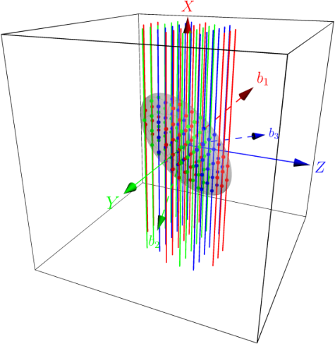
Implementing Fourier Transforms to and from the G-space using a single 3D FFT operation might not be optimal as some Fourier components can be ignored. By the definition of G-space, certain regions of the FFT grid are set to zero and this region is fixed for a given lattice and cutoff parameters. When computing the 3D FFT of let’s say a $N\times N\times N$ array, we can evaluate them with $N^{2}$ 1D FFT’s across each of the three axes. Knowing the truncated region, we can skip calling the actual 1D FFT routines on the 1D ‘sticks’ that contain no non-zero elements [39]. Figure (1), shows the G-space for the BCC Iron lattice. As can be seen in the figure, a large fraction of the elements are zero. In theory, this reduces the total number of FFT operations as long as the G-vectors are compactly grouped within the FFT Grid, which is the case when truncating with an energy cutoff. But, in practice, the implementation requires data to be rearranged between each 1D FFT calls. Also, 3D FFT implementations involve batched FFT calls where the library operates on multiple 1D arrays simultaneously. These two factors lowers the method’s overall efficiency and limits the algorithm effectiveness to only large grid sizes.

The runtime performance is sensitive to its implementation details and highly dependent on the structure of the G-space. But for wave-functions where the number of G-vectors is much smaller than the total number of FFT Grid points, this method reduces the computation involved in r2g()/g2r() methods.

Refer to caption — (a) G-Space in Cartesian coords

4.4 Data Containers: Buffers, Fields and Wavefun

For ease-of-use, we need to pair GSpace with a data container for representing and operating on with quantities like potentials, charge-density etc. that share the same periodicity as the crystal. A simple NumPy array would not be sufficient as it will not contain any data regarding the lattice and the G-space, which is required for many methods such as computing the Hartree potential, evaluating the del operator on a scalar/vector field, constructing the kinetic energy operator, etc. But, the container should mimic a lot of NumPy features like array slicing, indexing, broadcasting, list comprehension, etc. and binary operations like +, -, *, /, % etc.

Therefore, we have implemented the Buffer class that is a custom array-like container that enables the aforementioned functionalities. Initialized with a GSpace instance and NumPy array, it also provides FFT routines to convert between the two bases. The Buffer class is extended by the following pairs of classes:

•

FieldR and FieldG: Represents multidimensional fields
•

WavefunR and WavefunG: Represents single particle Bloch wavefunctions for a given k-point and stores its periodic part.

The Buffer base class implements the following methods:

•

copy(): creating copies of existing instances
•

empty(gspc, shape) and zeros(gspc, shape): Creating an empty/zero array with basis defined by gspc and input shape.
•

to_r() / to_g(): conversion from G-Space to R-Space and vice-versa via respectively.

Internally, Buffer supports a select set of NumPy functions that operate on one element of an array at a time. Called as Universal Functions in NumPy, they provide a wide range of routines of which the Buffer class supports the following:

•

Unary operations like computing trigonometric functions, negation, conjugation, logical/bit-wise inversion, etc.
•

Binary operations such as +, -, *, /, % and other algebraic, logical and bit-wise operations.
•

Reduction operations where one of the axes of the input array is reduced by repeatedly applying a binary operation to the values in array along the given axis.
•

Matrix multiplication (only across the last two dimensions of array(s))

To improve performance, the WavefunG implements the WavefunG.vdot(psi, phi) method for evaluating the dot product $\innerproduct{\psi_i}{\varphi_j}$ that directly calls the ZGEMM BLAS method in
scipy.linalg.blas module. This is to prevent calling ndarray.conj() method in NumPy that results in creating a new array and increasing memory usage.

⬇

def print_info(f):

typ = type(f)

basis = getattr(f, ’basis_type’, ’N\A’)

data = getattr(f, ’data’, None)

shape = data.shape if data is not None else ’N/A’

print(f"type: {str(type(f)):35}\n"

f"basis: ’{basis}’, data.shape: {shape}\n")

# Creating a empty GField instance

a_g = FieldG_gspc.empty((4, 10))

print_info(a_g)

## type: <class ’qtm.containers.field.get_FieldG.<locals>.FieldG’>

## basis: ’g’, data.shape: (4, 10, 2243)

# Converting to RField instance

a_r = a_g.to_r()

print_info(a_r)

References

- [1] P. Hohenberg and W. Kohn, Inhomogeneous electron gas, Phys. Rev. 136, B864 (1964), 10.1103/PhysRev.136.B864.
- [2] W. Kohn and L. J. Sham, Self-consistent equations including exchange and correlation effects, Phys. Rev. 140, A1133 (1965), 10.1103/PhysRev.140.A1133.
- [3] L. Hedin, New method for calculating the one-particle green’s function with application to the electron-gas problem, Phys. Rev. 139, A796 (1965), 10.1103/PhysRev.139.A796.
- [4] J. Deslippe, G. Samsonidze, D. A. Strubbe, M. Jain, M. L. Cohen and S. G. Louie, BerkeleyGW: A massively parallel computer package for the calculation of the quasiparticle and optical properties of materials and nanostructures, Computer Physics Communications 183(6), 1269 (2012), https://doi.org/10.1016/j.cpc.2011.12.006.
- [5] P. Giannozzi, S. Baroni, N. Bonini, M. Calandra, R. Car, C. Cavazzoni, D. Ceresoli, G. L. Chiarotti, M. Cococcioni, I. Dabo, A. D. Corso, S. de Gironcoli et al., QUANTUM ESPRESSO: a modular and open-source software project for quantum simulations of materials, Journal of Physics: Condensed Matter 21(39), 395502 (2009), 10.1088/0953-8984/21/39/395502.
- [6] P. Giannozzi, O. Andreussi, T. Brumme, O. Bunau, M. B. Nardelli, M. Calandra, R. Car, C. Cavazzoni, D. Ceresoli, M. Cococcioni, N. Colonna, I. Carnimeo et al., Advanced capabilities for materials modelling with quantum ESPRESSO, Journal of Physics: Condensed Matter 29(46), 465901 (2017), 10.1088/1361-648X/aa8f79.
- [7] X. Gonze, B. Amadon, G. Antonius, F. Arnardi, L. Baguet, J.-M. Beuken, J. Bieder, F. Bottin, J. Bouchet, E. Bousquet, N. Brouwer, F. Bruneval et al., The Abinit project: Impact, environment and recent developments, Comput. Phys. Commun. 248, 107042 (2020), https://doi.org/10.1016/j.cpc.2019.107042.
- [8] A. H. Romero, D. C. Allan, B. Amadon, G. Antonius, T. Applencourt, L. Baguet, J. Bieder, F. Bottin, J. Bouchet, E. Bousquet, F. Bruneval, G. Brunin et al., ABINIT: Overview, and focus on selected capabilities, J. Chem. Phys. 152, 124102 (2020), 10.1063/1.5144261.
- [9] G. Kresse and J. Furthmüller, Efficient iterative schemes for ab initio total-energy calculations using a plane-wave basis set, Phys. Rev. B 54, 11169 (1996), 10.1103/PhysRevB.54.11169.
- [10] L. Kronik, A. Makmal, M. L. Tiago, M. M. G. Alemany, M. Jain, X. Huang, Y. Saad and J. R. Chelikowsky, PARSEC – the pseudopotential algorithm for real-space electronic structure calculations: recent advances and novel applications to nano-structures, physica status solidi (b) 243(5), 1063 (2006), https://doi.org/10.1002/pssb.200541463, https://onlinelibrary.wiley.com/doi/pdf/10.1002/pssb.200541463.
- [11] N. Tancogne-Dejean, M. J. T. Oliveira, X. Andrade, H. Appel, C. H. Borca, G. Le Breton, F. Buchholz, A. Castro, S. Corni, A. A. Correa, U. De Giovannini, A. Delgado et al., Octopus, a computational framework for exploring light-driven phenomena and quantum dynamics in extended and finite systems, The Journal of Chemical Physics 152(12), 124119 (2020), 10.1063/1.5142502, https://doi.org/10.1063/1.5142502.
- [12] A. Castro, H. Appel, M. Oliveira, C. A. Rozzi, X. Andrade, F. Lorenzen, M. A. L. Marques, E. K. U. Gross and A. Rubio, octopus: a tool for the application of time-dependent density functional theory, physica status solidi (b) 243(11), 2465 (2006), https://doi.org/10.1002/pssb.200642067, https://onlinelibrary.wiley.com/doi/pdf/10.1002/pssb.200642067.
- [13] A. Marini, C. Hogan, M. Grüning and D. Varsano, yambo: An ab initio tool for excited state calculations, Computer Physics Communications 180(8), 1392 (2009), https://doi.org/10.1016/j.cpc.2009.02.003.
- [14] S. Curtarolo, W. Setyawan, G. L. Hart, M. Jahnatek, R. V. Chepulskii, R. H. Taylor, S. Wang, J. Xue, K. Yang, O. Levy, M. J. Mehl, H. T. Stokes et al., Aflow: An automatic framework for high-throughput materials discovery, Computational Materials Science 58, 218 (2012), https://doi.org/10.1016/j.commatsci.2012.02.005.
- [15] S. P. Huber, S. Zoupanos, M. Uhrin, L. Talirz, L. Kahle, R. Häuselmann, D. Gresch, T. Müller, A. V. Yakutovich, C. W. Andersen, F. F. Ramirez, C. S. Adorf et al., Aiida 1.0, a scalable computational infrastructure for automated reproducible workflows and data provenance, Scientific Data 7(1), 300 (2020), 10.1038/s41597-020-00638-4.
- [16] A. Jain, S. P. Ong, W. Chen, B. Medasani, X. Qu, M. Kocher, M. Brafman, G. Petretto, G. Rignanese, G. Hautier, D. Gunter and K. A. Persson, Fireworks: a dynamic workflow system designed for high-throughput applications, Concurrency and Computation: Practice and Experience 27(17), 5037–5059 (2015), 10.1002/cpe.3505.
- [17] M. Kruse, U. Petralanda, M. N. Gjerding, K. W. Jacobsen, K. S. Thygesen and T. Olsen, Two-dimensional ferroelectrics from high throughput computational screening, npj Computational Materials 9(1), 45 (2023), 10.1038/s41524-023-00999-5.
- [18] T. Biswas and A. K. Singh, pygwbse: a high throughput workflow package for gw-bse calculations, npj Computational Materials 9(1), 22 (2023), 10.1038/s41524-023-00976-y.
- [19] python/cpython the python programming language.
- [20] J. Ihm, A. Zunger and M. L. Cohen, Momentum-space formalism for the total energy of solids, Journal of Physics C: Solid State Physics 12(21), 4409 (1979).
- [21] M. S. Hybertsen and S. G. Louie, Electron correlation in semiconductors and insulators: Band gaps and quasiparticle energies, Phys. Rev. B 34, 5390 (1986), 10.1103/PhysRevB.34.5390.
- [22] L. Kleinman and D. M. Bylander, Efficacious form for model pseudopotentials, Phys. Rev. Lett. 48, 1425 (1982), 10.1103/PhysRevLett.48.1425.
- [23] E. Runge and E. K. U. Gross, Density-functional theory for time-dependent systems, Phys. Rev. Lett. 52, 997 (1984), 10.1103/PhysRevLett.52.997.
- [24] L. J. Sham and M. Schlüter, Density-functional theory of the energy gap, Phys. Rev. Lett. 51, 1888 (1983), 10.1103/PhysRevLett.51.1888.
- [25] J. P. Perdew and M. Levy, Physical content of the exact kohn-sham orbital energies: Band gaps and derivative discontinuities, Phys. Rev. Lett. 51, 1884 (1983), 10.1103/PhysRevLett.51.1884.
- [26] F. Aryasetiawan and O. Gunnarsson, The GW method, Reports on Progress in Physics 61(3), 237 (1998), 10.1088/0034-4885/61/3/002.
- [27] B. Holm and U. von Barth, Fully self-consistent self-energy of the electron gas, Phys. Rev. B 57, 2108 (1998), 10.1103/PhysRevB.57.2108.
- [28] S. B. Zhang, D. Tománek, M. L. Cohen, S. G. Louie and M. S. Hybertsen, Evaluation of quasiparticle energies for semiconductors without inversion symmetry, Phys. Rev. B 40, 3162 (1989), 10.1103/PhysRevB.40.3162.
- [29] J. Deslippe, G. Samsonidze, M. Jain, M. L. Cohen and S. G. Louie, Coulomb-hole summations and energies for calculations with limited number of empty orbitals: A modified static remainder approach, Phys. Rev. B 87, 165124 (2013), 10.1103/PhysRevB.87.165124.
- [30] PyPy: A fast, compliant alternative implementation of python, https://www.pypy.org/, Accessed: 2022-11-10.
- [31] S. K. Lam, A. Pitrou and S. Seibert, Numba: A LLVM-Based Python JIT Compiler, In Proceedings of the Second Workshop on the LLVM Compiler Infrastructure in HPC, LLVM ’15. Association for Computing Machinery, New York, NY, USA, ISBN 9781450340052, 10.1145/2833157.2833162 (2015).
- [32] Cython: C-extensions for python, https://cython.org/, Accessed: 2022-11-10.
- [33] C. R. Harris, K. J. Millman, S. J. van der Walt, R. Gommers, P. Virtanen, D. Cournapeau, E. Wieser, J. Taylor, S. Berg, N. J. Smith, R. Kern, M. Picus et al., Array programming with NumPy, Nature 585(7825), 357 (2020), 10.1038/s41586-020-2649-2.
- [34] R. Okuta, Y. Unno, D. Nishino, S. Hido and C. Loomis, CuPy: A NumPy-Compatible Library for NVIDIA GPU Calculations, In Proceedings of Workshop on Machine Learning Systems (LearningSys) in The Thirty-first Annual Conference on Neural Information Processing Systems (NIPS) (2017).
- [35] H. Gomersall, pyFFTW, 10.5281/zenodo.59508 (2016).
- [36] IntelPython/MKL_FFT: Numpy-based python interface to Intel (R) MKL FFT functionality.
- [37] P. Virtanen, R. Gommers, T. E. Oliphant, M. Haberland, T. Reddy, D. Cournapeau, E. Burovski, P. Peterson, W. Weckesser, J. Bright, S. J. van der Walt, M. Brett et al., SciPy 1.0: Fundamental Algorithms for Scientific Computing in Python, Nature Methods 17, 261 (2020), 10.1038/s41592-019-0686-2.
- [38] A. Stathopoulos and J. R. McCombs, PRIMME: PReconditioned Iterative MultiMethod Eigensolver: Methods and software description, ACM Transactions on Mathematical Software 37(2), 21:1 (2010).
- [39] A. Canning, Scalable parallel 3d ffts for electronic structure codes, In J. M. L. M. Palma, P. R. Amestoy, M. Daydé, M. Mattoso and J. C. Lopes, eds., High Performance Computing for Computational Science - VECPAR 2008, pp. 280–286. Springer Berlin Heidelberg, Berlin, Heidelberg, ISBN 978-3-540-92859-1 (2008).
- [40] Python array api standard.
- [41] D. R. Hamann, Optimized norm-conserving vanderbilt pseudopotentials, Phys. Rev. B 88, 085117 (2013), 10.1103/PhysRevB.88.085117.
- [42] P. E. Blöchl, Projector augmented-wave method, Phys. Rev. B 50, 17953 (1994), 10.1103/PhysRevB.50.17953.
- [43] D. Vanderbilt, Soft self-consistent pseudopotentials in a generalized eigenvalue formalism, Phys. Rev. B 41, 7892 (1990), 10.1103/PhysRevB.41.7892.
- [44] A. Willand, Y. O. Kvashnin, L. Genovese, Á. Vázquez-Mayagoitia, A. K. Deb, A. Sadeghi, T. Deutsch and S. Goedecker, Norm-conserving pseudopotentials with chemical accuracy compared to all-electron calculations, The Journal of Chemical Physics 138(10), 104109 (2013), 10.1063/1.4793260, https://doi.org/10.1063/1.4793260.
- [45] M. van Setten, M. Giantomassi, E. Bousquet, M. Verstraete, D. Hamann, X. Gonze and G.-M. Rignanese, The Pseudodojo: Training and grading a 85 element optimized norm-conserving pseudopotential table, Computer Physics Communications 226, 39 (2018), https://doi.org/10.1016/j.cpc.2018.01.012.
- [46] K. Lejaeghere, G. Bihlmayer, T. Björkman, P. Blaha, S. Blügel, V. Blum, D. Caliste, I. E. Castelli, S. J. Clark, A. D. Corso, S. de Gironcoli, T. Deutsch et al., Reproducibility in density functional theory calculations of solids, Science 351(6280), aad3000 (2016), 10.1126/science.aad3000, https://www.science.org/doi/pdf/10.1126/science.aad3000.
- [47] M. Schlipf and F. Gygi, Optimization algorithm for the generation of ONCV pseudopotentials, Computer Physics Communications 196, 36 (2015), https://doi.org/10.1016/j.cpc.2015.05.011.
- [48] D. D. Johnson, Modified broyden’s method for accelerating convergence in self-consistent calculations, Phys. Rev. B 38, 12807 (1988), 10.1103/PhysRevB.38.12807.
- [49] V. Eyert, A Comparative Study on Methods for Convergence Acceleration of Iterative Vector Sequences, Journal of Computational Physics 124(2), 271 (1996), 10.1006/jcph.1996.0059.
- [50] T. Rangel, M. Del Ben, D. Varsano, G. Antonius, F. Bruneval, F. H. da Jornada, M. J. van Setten, O. K. Orhan, D. D. O’Regan, A. Canning, A. Ferretti, A. Marini et al., Reproducibility in G0W0 calculations for solids, Computer Physics Communications 255, 107242 (2020), https://doi.org/10.1016/j.cpc.2020.107242.
- [51] Numerical data and functional relationships in science and technology: Photoemissions-Spektren und verwandte Daten. Teilbd. a / T. C. Chiang: Gruppe 3: Kristall- und Festkörperphysik = Group 3: @Crystal and solid state physics Bd. 23. Elektronische Struktur von Festkörpern, vol. 23, Springer, Berlin Heidelberg, ISBN 9783540500421 (1989).
- [52] E. L. Shirley, X. Zhu and S. G. Louie, Core polarization in solids: Formulation and application to semiconductors, Phys. Rev. B 56, 6648 (1997), 10.1103/PhysRevB.56.6648.
- [53] B. D. Malone and M. L. Cohen, Quasiparticle semiconductor band structures including spin–orbit interactions, Journal of Physics: Condensed Matter 25(10), 105503 (2013), 10.1088/0953-8984/25/10/105503.
- [54] F. Birch, Finite elastic strain of cubic crystals, Phys. Rev. 71, 809 (1947), 10.1103/PhysRev.71.809.
- [55] P. Blaha, K. Schwarz, G. Madsen, D. Kvasnicka and J. Luitz, WIEN2k, an augmented plane wave plus local orbitals program for calculating crystal properties (vienna university of technology, austria, 2001) (2002).
- [56] P. Blaha, K. Schwarz, F. Tran, R. Laskowski, G. K. H. Madsen and L. D. Marks, WIEN2k: An APW+lo program for calculating the properties of solids, Journal of Chemical Physics 152(7) (2020), 10.1063/1.5143061.
- [57] X. Qian, J. Li, X. Lin and S. Yip, Time-dependent density functional theory with ultrasoft pseudopotentials: Real-time electron propagation across a molecular junction, Phys. Rev. B 73, 035408 (2006), 10.1103/PhysRevB.73.035408.