The Ground-state Inter-plane Superconducting Coherence Length of La1.875Sr0.125CuO4 Measured by a “Xiometer”
Abstract
A long excitation coil piercing a superconducting (SC) ring is used to generate ever increasing persistent current in the ring, until the current destroys the order parameter. Given that the penetration depth is known, this experiment measures, hypothetically, the coherence length , hence the name ”Xiometer”. We examine various aspects of this theoretically driven hypothesis by testing niobium rings with different dimensions, and by comparing the results to the known values of . We then apply the method to two La1.875Sr0.125CuO4 rings at . In one, the current flows in the CuO2 planes hence it is set by . In the other, the current must cross planes and is determined by . We find that nm, and nm indicating that at low temperatures the Cooper pairs are three dimensional.
In the world of superconductivity there are two important length scales: the penetration depth , and the coherence length . From an application point of view, is a measure of superconducting carrier density and determines the current carrying capabilities of a superconductor, while sets the dimensions of Josephson junctions. There is an arsenal of experimental methods to directly measure the superconducting stiffness and find via the relation in different crystal orientations. However, methods of measuring are limited. In the cuprates the coherence length in the plane () was measured by: electron–boson spectral density function Hwang 2021 and vortex diameter via scanning tunneling microscopy (STM) Pan et al. 2000. More commonly, one finds near using one of various methods: resistivity Oh et al. 1988 vortex-Nernst effect Wang et al. 2003, specific heat Wang and Wen 2008, or thermal conductivity Grissonnanche et al. 2014, extrapolating to using theories that are not necessarily accurate over the whole temperature range, and uses the relation Oh et al. 1988; Petrenko et al. 2022. All methods find on the scale of nm.
Measuring coherence length in the direction () in cuprates is more difficult since it is smaller and because cleaving in a plane including the axis is challenging, making scanning techniques nearly impossible. is bound by nm, the thickness of a superconducting Bi2Sr2CaCu2O8+x (Bi2212) monolayer Yu et al. 2019. Extrapolations from high temperatures lead to Å Petrenko et al. 2022; Oh et al. 1988. The only measured value of nm at , as far as we know, is from an of T obtained using the electromagnetic flux compression method Sekitani et al. 2004. This number has been questioned due to the transient nature of the magnetic field. Exact determination of is becoming exceedingly important due to Josephson junctions created by twisted Bi2212 crystals Lee et al. 2022; Klemm 2005; Song et al. 2022; Lee et al. 2021; Takano et al. 2002 showing fractional Shapiro steps Zhao et al. 2021; Tummuru et al. 2022, and as a challenge for cuprates theory.
A new approach for measuring was suggested, and a very simple analysis formula was given, in Ref. [Gavish et al. 2021]. We name this approach “Xiometer”. Here we briefly present the approach, justify the formula intuitively, and test it on Nb. Then, we apply it to measurements in La1.875Sr0.125CuO4 (LSCO-1/8). We find that the nm determined by the Xiometer at is similar to the one obtained from T of Ref. Sekitani et al. 2004 and calculation in Ref. Petrenko et al. 2022. The implication of this finding is that the Cooper pairs are more spherical than previously thought.

The Xiometer, like the Stiffnessometer Mangel et al. 2020, is based on a long, current carrying, excitation coil (EC) piercing a superconducting (SC) ring and a measurement of the ring’s magnetic moment. The measurement is done by moving both ring and EC rigidly relative to a gradiometer type pick-up loops as demonstrated in Fig. 1(a). The gradiometer is connected to a superconducting quantum interference device (SQUID). The ring and EC are cooled to , only then the current in the EC is turned on, and the magnetic moment of the ring is measured. The gauge invariant London equation states that
| (1) |
where is the superconducting current density, is the total vector potential, is the flux quanta, and is the phase of the superconductor’s order parameter. is a combination of the EC vector potential , and the SC ring self induced vector potential .
To minimize the kinetic energy after cooling, the superconductor sets its own phase gradient to zero. Since this phase is quantized, turning the EC current on, gently, conserve the phase. Therefore, at the start of a measurement, the London equation is valid. In principle, this relation can be used to determine the stiffness and in this case the apparatus works as a Stiffnessometer. However, for bulk crystals at low temperatures, when is mach smaller than all dimensions of the sample, the SC ring exactly expels the applied flux, to keep deep inside the ring, regardless of . In this case, the apparatus cannot be used to properly determine the stiffness, but only the break point of the London equation, which is set by as we explain below. For crystals at we use literature values of and determine . Hence, the name Xiometer.
The EC is home made from a NbTi SC wire with: layers of windings each ( in total), a wire diameter mm, core diameter mm, outer diameter mm, coil length mm, and flux to current ratio of . The apparatus is an add-on to a Cryogenics S700X SQUID magnetometer. External magnetic fields can be canceled by an external coil shown in Fig. 1(a), with a resolution of T. The gradiometer radius is mm, its total height is mm, and it is made of: two windings clockwise, four anticlockwise, and two clockwise also depicted in Fig. 1(a). The set of Nb rings with different dimensions used in the first part of this experiment is shown in Fig. 1(b).
A typical data set of the SQUID output voltage as a function of ring position , is depicted in Fig. 2 with and without a ring. In these measurements the EC was allowed to transverse the gradiometer from one side to the next. The peaks and valleys away from are due to the ends of the coil moving through the different winding groups of the gradiometer. Without the ring (red symbols) a moderately concave signal is observed around . This occurs when the center of the gradiometer and the center of the coil are at the same height. In this situation, flux through the gradiometer due to the EC barely changes, therefore the measurement is sensitive mostly to . With the ring, a new signal (blue symbols) appears around . The difference is the net SC ring’s signal (inset) and its amplitude is proportional to the magnetic moment (or ) of the ring. We note that a linear base-line was subtracted from both data sets due to the EC asymmetry (wires enter and exit from one side only). Linear base-line subtraction is irrelevant for the data analysis (see below).
As the EC current increases, the signal from the EC traversing the gradiometer overwhelms the ring’s signal, as is clear from Fig. 3. Therefore, we limit the motion to a small region around . Consequently it is impossible to detect the bottom of the signal and evaluate its amplitude. However, it is clear that the top of the peak at becomes sharper with increasing current. Therefore, we use the second derivative of the SQUID’s output voltage as a measure of . This method also eliminates the undesired linear contribution of the coil’s asymmetry. The conversion from to is explained shortly.
Finally, to keep the leads, coil, and ring cooled, liquid helium is sprayed via a diffuser from the bottom of the sample chamber on the EC and sample, and pumped along the current leads all the way to the top of the cryostat just before thicker leads are connected to the power supply. This way the EC remains cold even when currents of more than A are applied.


The measured samples are pure Nb rings, and two LSCO- single crystal rings, grown, using a traveling solvent floating zone technique and cut with a laser cutter. Laue x-ray diffraction is used to identify the orientation of the crystals and the two rings are cut in different orientations of the CuO2 planes relative to ring’s symmetry axis. In one ring the CuO2 planes are parallel to the symmetry axis. In the other ring the planes are perpendicular to this axis. We address the two rings as and rings, respectively. In the ring, current can flow around the ring on CuO2 planes without crossing planes. In order to flow around the ring current must cross CuO2 planes.
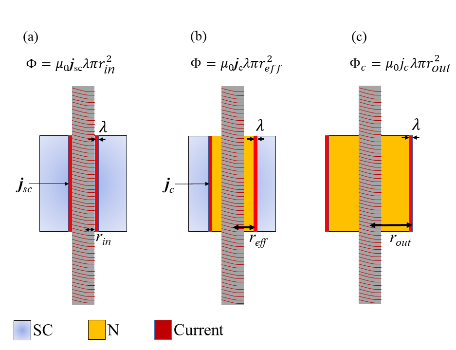
A detailed derivation of the Xiometer analysis theory can be found in Ref. Gavish et al. 2021. Here we provide a back of the envelope calculation that gives the same answer up to a numerical factor. Since, as mentioned before, deep in the superconductor there are no currents (and no fields), . Therefore, the magnetic flux of the EC, , is perfectly matched by the magnetic flux from the super-current in the ring, namely, . For low we assume that the supper current density is uniform along a cylinder of width attached to the inner rim of the ring at as in Fig. 4(a). The magnetic flux of such a current is . When increases, will also increases until it reaches the critical current density of the SC. When this happens the order parameter is destroyed next to the inner rim, and the current has to retreat from the inner rim to an effective radius demonstrated in Fig. 4(b). This process continues until as shown in Fig. 4(c). At this situation vortices start entering the sample, and the applied flux is named critical flux; it is given by . Using the definition where , , , and are the carrier’s density, velocity, charge, and mass respectively, and the relations of the critical momentum Tinkham 2004, and the flux quanta one finds
| (2) |
where . In the exact derivation Gavish et al. 2021 .
It should be pointed out that the SC produce a field in the volume where the order parameter is destroyed. One might wonder if this field penetrates as vortices into the SC when it is of Type-II. It was found in Ref. Khanukov et al. 2022, using a scanning SQUID, that in ultra thin film that show vortices due to sporadic magnetic field, the current in the coil does not add new vortices. This is not surprising since there is no pressure from twisted field lines bypassing the sample to penetrate into the sample. In our case the field lines are strait and in the center of the sample. They are in the most convenient place to be and do not need to penetrate the sample as vortices.

The output voltage of the SQUID is related to the flux through the gradiometer by where is a conversion factor. When a sample with magnetic moment is located at height from the center of a single pickup-loop with radius , it’s flux through the loop is . To calibrate we measured our coil for which we calculate the magnetic moment as a bundle of current loops with moment each, where is the loop radius. The voltage output in this case is:
| (3) |
where is the distance between the center of the coil and the center of the gradiometer, is the difference between the gradiometer’s bundles, is the radius of the ’th layer, and the height of the ’th loop. By fitting Eq. 3 to a measurement of the coil with current of , as shown in Fig. 2, we find the conversion factor to be V/Tmm2. This procedure gives
| (4) |
where is in units of mV/mm2, and in units of Am2.
To test Eq. 2 we measure a set of Nb rings with different inner and outer radii, and different height. Fig. 5 presents as a function of the applied EC current . is linear for low currents. At some high current , a jump in is observed indicating that the critical flux in the coil is reached, and that a phase slip has taken place. This process was done more than once for each ring for better statistics.
The results of the experiment with the Nb rings is separated to three sets. In each set only one parameter is changing: inner radius panel (a), outer radius panel (b), and the ring’s height panel (c). Variation of is limited because of the coil. Nevertheless, it does not seem to impact the . Variation of has noticeable and systematic influence on the critical flux as expected from Eq. 2. Finally, between the smallest mm and all other values of a variation in is detected. This is not expected from Eq. 2. We ascribe this exception to the fact that Eq. 2 is derived in the limit of a tall, cylinder like, ring and the mm is not in this limit. A summary of as a function of () is depicted in the inset of Fig. 6 where it is clear that is the most important parameter. The error bars are statistical.
In Fig. 6 we present the dependence of on a full scale including the origin. When taking and of Nb as nm and nm respectively from Ref. [Maxfield and Mclean 1965] and applying those in Eq. 2 (black line), we find reasonable agreement between the measurements and theory. When fitting Eq. 2 to the data (red line), we find nm2 while the literature value is nm2.


Having established Eq. 2 we use it to measure coherence length of the two LSCO- rings shown in the insets of Fig. 7 with orientation and planes illustrated in the main panel. Previously, it was found that the persistent current critical temperature for the c-ring is higher than for the a-ring Kapon et al. 2019. Figure. 7 shows at K as function of EC current for both the a-, and c-rings. At low currents, is linear for both rings. But at about A, the a-ring moment has a break point where its behaviour changes. The c-ring moment stays linear all the way up to our maximum current of A. We interpret this break point as the critical flux where vortices start entering the sample. [floatfix] At the experiment’s temperature, the penetration depths of LSCO with are: nm [Panagopoulos et al. 2000], and nm [Kapon et al. 2019]. The outer radii of the a- and c-rings are mm, and mm. Following Eq. 2 with we find nm. The assumption here is that the bottleneck for current in the a-ring is the flow between planes (c-direction), and that the order parameter is destroyed first on the planes perpendicular to the flow. We can also place an upper bound on nm using .
The Ginzburg–Landau at , which we measure with the Xiometer, is related to the Cooper pair size by a factor of 0.74 Tinkham 2004. , in turn, is set by where is the Fermi velocity and delta is the superconducting gap. However, in the cuprates varies along the Fermi surface, in the direction is not known, and there is no theory that can be used to extract more fundamental properties or be contrasted with our findings. A derivation of such a theory could be useful.
To summarize, the relation between the dimensions of a superconducting ring, pierced by a long coil, and the critical flux in the coil, is tested. It is demonstrated that if the ring’s height is similar to or bigger than its radii, only the outer radius of the ring is relevant, and the critical flux depends quadratically on this radius. Using this observation we measured and of LSCO- at K. Despite the cuprates being very unisotropic systems, we found that is similar to the literature value of , indicating a 3D Cooper pair.
Acknowledgements
This research was funded by the Israeli Science foundation grant number 3875/21.
References
- Hwang (2021) J. Hwang, Scientific Reports — 11, 11668 (2021).
- Pan et al. (2000) S. H. Pan, E. W. Hudson, A. K. Gupta, K.-W. Ng, H. Eisaki, S. Uchida, and J. C. Davis, Phys. Rev. Lett. 85, 1536 (2000).
- Oh et al. (1988) B. Oh, K. Char, A. D. Kent, M. Naito, M. R. Beasley, T. H. Geballe, R. H. Hammond, A. Kapitulnik, and J. M. Graybeal, Phys. Rev. B 37, 7861 (1988).
- Wang et al. (2003) Y. Wang, S. Ono, Y. Onose, G. Gu, Y. Ando, Y. Tokura, S. Uchida, and N. P. Ong, Science 299, 86 (2003).
- Wang and Wen (2008) Y. Wang and H.-H. Wen, EPL (Europhysics Letters) 81, 57007 (2008).
- Grissonnanche et al. (2014) G. Grissonnanche, O. Cyr-Choinière, F. Laliberté, S. R. de Cotret, A. Juneau-Fecteau, S. Dufour-Beauséjour, M. Ã. Delage, D. LeBoeuf, J. Chang, B. J. Ramshaw, D. A. Bonn, W. N. Hardy, R. Liang, S. Adachi, N. E. Hussey, B. Vignolle, C. Proust, M. Sutherland, S. Kr�mer, J. H. Park, D. Graf, N. Doiron-Leyraud, and L. Taillefer, Nat. Commun. 5 (2014).
- Petrenko et al. (2022) Â. E. V. Petrenko, L. V. Omelchenko, A. V. Terekhov, Y. A. Kolesnichenko, K. Rogacki, D. M. Sergeyev, A. L. Solovjov, and E. V. Petrenko, Low Temperature Physics 48, 755 (2022).
- Yu et al. (2019) Y. Yu, L. Ma, P. Cai, R. Zhong, C. Ye, J. Shen, G. D. Gu, X. H. Chen, and Y. Zhang, Nature 2019 575:7781 575, 156 (2019).
- Sekitani et al. (2004) T. Sekitani, N. Miura, S. Ikeda, Y. H. Matsuda, and Y. Shiohara, Physica B: Condensed Matter 346-347, 319 (2004).
- Lee et al. (2022) Y. Lee, M. Martini, T. Confalone, S. Shokri, C. N. Saggau, G. Gu, K. Watanabe, T. Taniguchi, D. Montemurro, V. M. Vinokur, K. Nielsch, and N. Poccia 10.48550/arxiv.2210.02124 (2022).
- Klemm (2005) R. A. Klemm, Philosophical Magazine 85, 801 (2005).
- Song et al. (2022) X.-Y. Song, Y.-H. Zhang, and A. Vishwanath, Physical Review B 105, L201102 (2022).
- Lee et al. (2021) J. Lee, W. Lee, G.-Y. Kim, Y.-B. Choi, J. Park, S. Jang, G. Gu, S.-Y. Choi, G. Y. Cho, G.-H. Lee, and H.-J. Lee, Nano Letters 21, 10469 (2021).
- Takano et al. (2002) Y. Takano, T. Hatano, A. Fukuyo, A. Ishii, M. Ohmori, S. Arisawa, K. Togano, and M. Tachiki, Physical Review B 65, 140513 (2002).
- Zhao et al. (2021) S. Y. F. Zhao, N. Poccia, X. Cui, P. A. Volkov, H. Yoo, R. Engelke, Y. Ronen, R. Zhong, G. Gu, S. Plugge, T. Tummuru, M. Franz, J. H. Pixley, and P. Kim 10.48550/arxiv.2108.13455 (2021).
- Tummuru et al. (2022) T. Tummuru, S. Plugge, and M. Franz, Physical Review B 105, 064501 (2022).
- Gavish et al. (2021) N. Gavish, O. Kenneth, and A. Keren, Physica D: Nonlinear Phenomena 415, 132767 1 (2021).
- Mangel et al. (2020) I. Mangel, I. Kapon, N. Blau, K. Golubkov, N. Gavish, and A. Keren, Phys. Rev. B 102, 024502 1 (2020).
- Tinkham (2004) M. Tinkham, Introduction to Superconductivity: v. 1 (Dover Publications Inc., 2004).
- Khanukov et al. (2022) A. Khanukov, I. Mangel, S. Wissberg, A. Keren, and B. Kalisky, PHYSICAL REVIEW B 106, 144510 (2022).
- Maxfield and Mclean (1965) B. W. Maxfield and W. L. Mclean, Phys. Rev. 139, A1515 (1965).
- Kapon et al. (2019) I. Kapon, Z. Salman, I. Mangel, T. Prokscha, N. Gavish, and A. Keren, Nat. Commun. 10 (2019).
- Panagopoulos et al. (2000) C. Panagopoulos, J. R. Cooper, T. Xiang, Y. S. Wang, and C. W. Chu, Phys. Rev. B 61, 163 (2000).
*
