Unified Lagrangian for Tachyon, Quintessence, and Phantom Scalar Fields

Tanisha Joshi Thanks: Tanisha.11919253@lpu.in Affiliation: Department of Physics, School of Chemical Engineering & Physical Sciences, Affiliation: Lovely Professional University, Phagwara, Punjab, 144411, India

25 July 2023

Abstract

This paper presents a novel unified Lagrangian density that combines the behaviors of tachyon, quintessence, and phantom scalar fields within the realms of theoretical physics and cosmology. The unified Lagrangian is formulated, where $f(\alpha)$ is a function that accommodates different scenarios and captures the distinct characteristics of these scalar fields. The potential function $V(\phi)$ is incorporated to account for the specific properties of the scalar fields. The study employs numerical simulations in Python to thoroughly analyze the dynamics of the scalar fields for various $\alpha$ values, investigating the cosmological behavior.

Keywords : Scalar fields, Unified Lagrangian, Tachyon, Quintessence, Phantom, dark energy, Scale Factor Evolution, Age of the Universe, Cosmological Dynamics

1 Introduction

The discovery of the universe’s accelerated expansion was a groundbreaking moment in cosmology. Prior to the late 1990s, it was widely believed that the universe’s expansion, initially observed by Edwin Hubble [1] in the 1920s, was gradually slowing down due to gravity’s attractive force. However, precise measurements of distant supernovae by two independent research teams [2, 3], the Supernova Cosmology Project and the High-Z Supernova Search Team, revealed a surprising result: the expansion was actually accelerating. This revelation presented a profound challenge to existing cosmological models and led to the postulation of dark energy—a mysterious and dominant form of energy that constitutes around $69\%$ of the total energy content of the universe.
Dark energy’s intriguing feature is its negative pressure, in contrast to ordinary matter’s positive pressure and gravitational attraction. This negative pressure exerts a repulsive gravitational effect, driving galaxies and cosmic structures apart at an ever-increasing rate. As a result, the universe’s expansion accelerates over time, giving rise to a dynamic and rapidly evolving cosmos. Despite its crucial role in shaping the universe’s large-scale structure and evolution, the fundamental nature of dark energy remains elusive, and it remains unaccounted for in the standard model of particle physics.
Scalar fields have emerged as a promising avenue for modeling dark energy due to their simplicity and versatility. A scalar field is described by a single scalar quantity that dynamically evolves in space and time, giving rise to various forms of dark energy, each with distinct properties and implications for the universe’s expansion. One such model is the quintessence field [5, 6, 7, 8, 9, 10, 11, 12], characterized by a slowly varying scalar field with positive kinetic energy and negative potential energy. As the universe expands, the quintessence field evolves, and its energy density decreases more slowly than ordinary matter or radiation. This leads to the gradual dominance of the quintessence field, resulting in the acceleration of the universe’s expansion. The dynamics of quintessence can be described by a scalar field potential, which determines how the energy density changes with the field’s value, offering various cosmic expansion histories that can be compared with observational data for testing the viability of the quintessence model.
Conversely, the phantom field [13] represents another scalar field model within the broader category of dark energy models. Unlike quintessence, the phantom field exhibits negative kinetic energy and a potential that steeply increases with the scalar field value. This peculiar characteristic yields an equation of state with $w<-1$ , where $w$ represents the ratio of pressure to energy density. The negative value of w leads to an even stronger repulsive gravitational effect compared to quintessence, driving the universe’s expansion to accelerate even more rapidly. The presence of the phantom field can result in intriguing cosmological consequences, including the possibility of future singularities known as ”Big Rip.”
Additionally, tachyon fields [14, 15, 16, 17] have been considered as potential dark energy candidates. Tachyons are scalar fields with imaginary mass, suggesting that they can never be at rest and always move faster than light. Despite this seemingly counter-intuitive property, tachyonic dark energy models have been proposed, wherein the tachyon field drives accelerated expansion. These models involve complex dynamics and necessitate careful scrutiny to ensure their consistency with observational data and theoretical constraints.
While individual scalar field models—quintessence, phantom, and tachyon—have been extensively studied in the context of dark energy, a unified framework encompassing the collective behavior of these scalar fields remains relatively unexplored. Such a unified approach seeks to identify common features, underlying principles, and potential connections between different scalar field models. Developing such a framework could potentially unveil deeper insights into the nature of dark energy and provide a more comprehensive understanding of its role in the accelerated expansion of the universe. This pursuit of a unified framework for scalar field-based dark energy models represents a crucial step towards solving the enigma of dark energy and unraveling one of the most significant mysteries in modern cosmology.
The motivation for a unified Lagrangian arises from several key factors. Firstly, a unified approach allows for a comprehensive analysis of scalar field behavior, enabling researchers to systematically explore how different types of scalar fields interact and collectively influence the Universe’s evolution. By bridging the gap between individual Lagrangians, a unified formulation ensures continuous and consistent descriptions of scalar field dynamics. Moreover, scalar fields are intricately related to fundamental forces and energy content in the Universe. A unified Lagrangian provides a coherent framework for studying these fields, shedding light on their roles in governing cosmic dynamics and their interactions with other particles and fields.
The quest for a unified Lagrangian is particularly relevant to understanding dark energy and cosmic acceleration, as these phenomena remain significant cosmological mysteries. By incorporating the diverse behaviors of tachyonic, quintessence, and phantom scalar fields, a unified approach can offer insights into the nature of dark energy and its potential connections to cosmic inflation and other cosmological processes. Ensuring consistency and coherence in scalar field descriptions is critical for constructing robust theoretical models that can be tested against observational data. A unified Lagrangian facilitates internal consistency, enabling researchers to make more accurate predictions and interpretations.
Developing a unified Lagrangian is not only scientifically valuable but also practically significant. It streamlines the theoretical framework, reducing complexity and redundancy in modeling scalar fields separately. This unified approach enhances the efficiency of numerical simulations and theoretical predictions, enabling researchers to explore a wider range of cosmological scenarios. This unified approach facilitates direct comparisons between different scalar field models, enabling us to identify common patterns, unique features, and the impact of various parameter values. Moreover, a unified Lagrangian allows for the exploration of emergent phenomena that arise from the interactions between scalar fields, leading to new insights into the dynamics of the universe. The pursuit of a unified Lagrangian for scalar fields holds immense potential for advancing our understanding of the fundamental nature of the cosmos.
The paper is structured into six sections, each serving a specific purpose to advance the study’s objectives. Section 1 serves as the introduction, providing essential background information and outlining the motivations driving the research. Section 2 delves into a comprehensive mathematical analysis of the unified Lagrangian, which governs the dynamic behavior of the scalar fields within the theoretical framework. Dedicated to stability analysis, Section 3 examines the behavior and stability of the scalar field dynamics. In Section 4, the paper conducts behavior analysis through numerical simulations, exploring various scenarios and values of the parameter $\alpha$ . Section 5 presents and discusses the results obtained from applying the unified framework to the cosmological dynamics of the scalar fields. Finally, Section 6 concludes the paper by summarizing the findings and implications of the study.

2 Mathematical Background

The Lagrangian formalism is a powerful mathematical framework used in classical mechanics and field theory to describe the dynamics of physical systems. It provides a concise and elegant way to describe the dynamics of fields in various physical theories, including classical field theories like electromagnetism and general relativity, as well as quantum field theories used in particle physics. It has proven to be a fundamental tool in understanding the behavior of physical systems and is widely used in theoretical physics research.
In this study, we made the assumption of a flat Friedmann-Lemaître-Robertson-Walker (FLRW) universe. Also, The Friedmann equations [18] are fundamental equations in cosmology that describe the evolution of the universe on a large scale. The FLRW metric [19, 20, 21, 22] is a fundamental framework in modern cosmology used to describe the large-scale structure and evolution of the universe. The cosmological principle [23, 24, 25], which has been widely supported by empirical evidence [26] and is considered highly robust [27, 28, 29], asserts the validity of a homogeneous and isotropic universe at large scales. By assuming a flat FLRW universe, we simplify the mathematical description of the cosmological model and obtain a clear and tractable framework for studying the dynamics of scalar fields and their interactions with the expansion of space. This assumption is widely used in cosmological studies and has provided a robust foundation for our understanding of the large-scale structure and evolution of the universe. Moreover, observations from cosmic microwave background radiation and large-scale galaxy surveys have supported the notion of a flat universe, further justifying its adoption in our analysis.
To derive the unified Lagrangian density for tachyon, quintessence, and phantom fields, we start by considering the Lagrangian densities of each individual scalar field and then introduce a function $f(\alpha)$ to unify their behaviors.
For the tachyon field, the Lagrangian density is given as :

L_{\text{tachyon}}=-V(\phi)\sqrt{1+\partial_{\mu}\phi\partial^{\mu}\phi}

(1)

For the Quintessence field, the Lagrangian density is given as :

L_{\text{quintessence}}=\frac{1}{2}\partial_{\mu}\phi\partial^{\mu}\phi-V(\phi)

(2)

For the Phantom field, the Lagrangian density is given as :

L_{\text{phantom}}=-V(\phi)\sqrt{1-\partial_{\mu}\phi\partial^{\mu}\phi}

(3)

Now, we define the function $f(\alpha)$ to capture the different behaviors of the scalar fields as :

f(\alpha)=\frac{1}{2}(1+\alpha)

(4)

The unified Lagrangian density $L_{\text{unified}}$ is given as :

L_{\text{unified}}=f(\alpha)\partial_{\mu}\phi\partial^{\mu}\phi-V(\phi)\sqrt{1-\alpha\partial_{\mu}\phi\partial^{\mu}\phi}

(5)

The unified Lagrangian is inherently nonlinear due to the presence of the square root term and the multiplication of the kinetic and potential energy contributions. This nonlinearity arises from the nature of the scalar field dynamics and the interplay between the kinetic and potential energy terms. The square root term $\sqrt{1-\alpha\partial_{\mu}\phi\partial^{\mu}\phi}$ introduces nonlinearity into the Lagrangian, as it depends on the derivative of the scalar field $\partial_{\mu}\phi\partial^{\mu}\phi$ . This nonlinearity can give rise to interesting and complex dynamics, allowing for a rich variety of solutions and behaviors of the scalar field. The Lagrangian also contains $\alpha$ -dependent coefficients through the function $f(\alpha)$ . The Lagrangian combines both kinetic and potential energy terms, influencing the overall dynamics and energy contributions.
The motivation for choosing the specific functional form $f(\alpha)=\frac{1}{2}(1+\alpha)$ in the unified Lagrangian stems from the need to develop a comprehensive framework that can effectively represent and differentiate the behaviors of tachyon, quintessence, and phantom fields. This choice of function is designed to capture the distinct characteristics exhibited by each scalar field while ensuring a coherent and consistent approach in theoretical physics and cosmology. The function $f(\alpha)$ depends on the parameter $\alpha$ , which allows us to modulate the behavior of the scalar fields. By varying the value of $\alpha$ , we can seamlessly transition between the different scalar field cases and study their individual dynamics within the same unified framework. This approach is crucial for exploring the interplay between these scalar fields and understanding their collective impact on cosmological evolution.
Let’s discuss the significance of this choice and its influence on the dynamics and behavior of the scalar fields:
1. Tachyon field ( $\alpha=-1$ ): When $\alpha$ takes the value of -1, the function $f(\alpha)$ evaluates to $f(-1)=\frac{1}{2}(1+(-1))=0$ . This implies that the Lagrangian density for the tachyon field does not include the kinetic term ( $\partial_{\mu}\phi\partial^{\mu}\phi$ ). It captures the unique feature of tachyon fields being tachyonic, characterized by negative kinetic energy and an imaginary mass.
2.Quintessence field ( $\alpha=0$ ): For the quintessence field, when $\alpha$ equals 0, the function $f(\alpha)$ becomes $f(0)=\frac{1}{2}(1+0)=\frac{1}{2}$ . In this case, the Lagrangian density includes both the kinetic term ( $\partial_{\mu}\phi\partial^{\mu}\phi$ ) and the potential term ( $V(\phi)$ ), as expected for quintessence fields. The chosen functional form accurately represents the behavior of quintessence fields as scalar fields with positive energy density and a wide range of possibilities for the equation of state.
3. Phantom field ( $\alpha=1$ ): When $\alpha$ takes the value of 1, the function $f(\alpha)$ evaluates to $f(1)=\frac{1}{2}(1+1)=1$ . This implies that the Lagrangian density for the phantom field includes both the kinetic term ( $\partial_{\mu}\phi\partial^{\mu}\phi$ ) and the potential term ( $V(\phi)$ ), but with a crucial difference. The presence of the square root in the potential term leads to a negative energy density, resulting in exotic phenomena associated with phantom fields such as super-acceleration and violation of the energy conditions.
Overall, the parameter $\alpha$ governs the contribution of the kinetic and potential terms in the Lagrangian, affecting the energy density, pressure, and equation of state of the scalar field. The value of $\alpha$ determines the stability, oscillatory behavior, and violation of energy conditions exhibited by the scalar field.
Let’s check the accuracy of the derivation for the unified Lagrangian densities:
1. Tachyon field ( $\alpha$ = -1): Starting with the unified Lagrangian:

L_{\text{unified}}=f(\alpha)\partial_{\mu}\phi\partial^{\mu}\phi-V(\phi)\sqrt{1-\alpha\partial_{\mu}\phi\partial^{\mu}\phi}

Substituting $\alpha$ = -1 in the unified Lagrangian :

L_{\text{unified}}=f(-1)\partial_{\mu}\phi\partial^{\mu}\phi-V(\phi)\sqrt{1-(-1)\partial_{\mu}\phi\partial^{\mu}\phi}

Now, $f(-1)=\frac{1}{2}(1-(-1))=0$ , and the expression simplifies to:

L_{\text{tachyon\_unified}}=V(\phi)\sqrt{1+\partial_{\mu}\phi\partial^{\mu}\phi}

(6)

This Lagrangian captures the unique feature of tachyon fields being tachyonic, characterized by negative kinetic energy and an imaginary mass.

Negative Kinetic Energy: In the Lagrangian, the term $\partial_{\mu}\phi\partial^{\mu}\phi$ appears with a positive sign inside the square root. Since the square root is taken over $1+\partial_{\mu}\phi\partial^{\mu}\phi$ , this means that the term $\partial_{\mu}\phi\partial^{\mu}\phi$ contributes to a negative sign under the square root. Hence, the kinetic energy of the tachyon field is negative, which is a key characteristic of tachyonic fields.

Imaginary Mass: For a scalar field with the standard canonical kinetic term $\frac{1}{2}\partial_{\mu}\phi\partial^{\mu}\phi$ , the mass term in the equation of motion is proportional to $\partial^{2}V/\partial\phi^{2}$ , where $V(\phi)$ is the potential. However, in the tachyon field Lagrangian, the presence of the square root term $\sqrt{1+\partial_{\mu}\phi\partial^{\mu}\phi}$ modifies the mass term. This results in an imaginary mass for the tachyon field, which is a distinct characteristic of tachyonic fields.
2. Quintessence field ( $\alpha$ = 0): Substituting $\alpha$ = 0 in the unified Lagrangian:

L_{\text{unified}}=f(0)\partial_{\mu}\phi\partial^{\mu}\phi-V(\phi)\sqrt{1-0\partial_{\mu}\phi\partial^{\mu}\phi}

Now, $f(0)=\frac{1}{2}(1+0)=\frac{1}{2}$ , and the expression becomes:

L_{\text{quintessence\_unified}}=\frac{1}{2}\partial_{\mu}\phi\partial^{\mu}\phi-V(\phi)

(7)

3. Phantom field ( $\alpha$ = 1): Substituting $\alpha$ = 1 in the unified Lagrangian:

L_{\text{unified}}=f(1)\partial_{\mu}\phi\partial^{\mu}\phi-V(\phi)\sqrt{1-1\partial_{\mu}\phi\partial^{\mu}\phi}

Now, $f(1)=\frac{1}{2}(1+1)=1$ , and the expression simplifies to:

L_{\text{phantom\_unified}}=\partial_{\mu}\phi\partial^{\mu}\phi-V(\phi)\sqrt{1-\partial_{\mu}\phi\partial^{\mu}\phi}

(8)

These equations represent the unified Lagrangian densities for the tachyon, quintessence, and phantom scalar fields, respectively, after substituting the appropriate terms and parameters. We derived a unified Lagrangian density $L_{\text{unified}}$ that combines the behaviors of tachyon, quintessence, and phantom scalar fields. The function $f(\alpha)$ allows for a consistent description, encompassing the distinct properties of each scalar field within a single unified framework. This unified formulation allows for a comprehensive description of the dynamics of these scalar fields within a single framework, providing insights into the behavior of the universe and its evolution.

2.1 Motivation for different Potentials Used

The motivations for using various potentials in this study are rooted in their relevance to theoretical physics, cosmological models, and their ability to capture different aspects of scalar field dynamics. Each potential serves a specific purpose and helps explore distinct cosmological scenarios and emergent phenomena. Below are the motivations for the potentials used:

1. Quadratic Potential : The quadratic potential is one of the simplest and well-studied potentials in theoretical physics. It is particularly relevant for describing inflationary scenarios, as it leads to slow-rolling behavior of the scalar field, resulting in a nearly constant energy density and inflationary expansion. The quadratic potential is commonly used in inflationary models due to its ability to address the horizon problem, flatness problem, and the generation of primordial density perturbations that seed the formation of large-scale structures in the universe.

2. Quartic Potential : The quartic potential represents a simple and mathematically tractable potential with a quartic dependence on the scalar field. It is often employed to study scenarios where the scalar field undergoes oscillatory behavior, damping down over time as the universe expands. The quartic potential can lead to interesting dynamics, including the possibility of multiple field oscillations and resonances, which can be relevant for understanding the field’s role in particle physics and early universe cosmology.

3. Exponential Potential : The exponential potential is frequently associated with scenarios involving dark energy or late-time accelerated expansion of the universe. It possesses an exponential dependence on the scalar field, leading to negative pressure and driving accelerated expansion in the late universe. The exponential potential is of particular interest for understanding the cosmic acceleration observed through supernovae and cosmic microwave background data.

4. Cosine Potential : The cosine potential is another commonly used potential in cosmology, often associated with axion-like fields. It leads to periodic oscillations of the scalar field, which can have implications for the behavior of dark matter or other axion-like particles. The cosine potential is relevant for understanding the dynamics of scalar fields in the early and late universe, and its periodic nature can lead to interesting cosmological features.

5. Power-Law Potential : The power-law potential is a versatile potential that covers a wide range of behaviors depending on the value of the exponent $n$ . For certain values of $n$ , the power-law potential can lead to chaotic or rapid oscillatory behavior of the scalar field, influencing the universe’s dynamics accordingly. The power-law potential is often used to explore a broad spectrum of cosmological scenarios, from early universe inflation to late-time cosmological evolution.

The choice of potentials in this study is motivated by their relevance to cosmological scenarios and their ability to capture distinct behaviors of scalar fields. Each potential serves as a mathematical representation of the scalar field’s energy in terms of its field value $\phi$ , and the specific form of the potential significantly influences the dynamics of the scalar field and its interaction with the expansion of the universe.

2.2 Scalar Field Dynamics

The Lagrangian density for the scalar field $\phi$ given by:

L_{\text{unified}}=f(\alpha)\partial_{\mu}\phi\partial^{\mu}\phi-V(\phi)\sqrt{1-\alpha\partial_{\mu}\phi\partial^{\mu}\phi}

(9)

The action for the given Lagrangian $L_{\text{unified}}$ is obtained by integrating the Lagrangian density over spacetime. The action $S$ is given by:

S=\int d^{4}x\sqrt{-g}\,L_{\text{unified}}

(10)

where $d^{4}x$ represents the spacetime volume element, $\sqrt{-g}$ is the determinant of the metric tensor $g_{\mu\nu}$ .

So, the action $S$ for the Lagrangian $L_{\text{unified}}$ is:

S=\int d^{4}x\sqrt{-g}\,\left(f(\alpha)\partial_{\mu}\phi\partial^{\mu}\phi-V(\phi)\sqrt{1-\alpha\partial_{\mu}\phi\partial^{\mu}\phi}\right)

(11)

Next, we will investigate the dynamics of the scalar fields for each case of $f(\alpha)$ and $\alpha$ in the unified Lagrangian $L_{\text{unified}}$ .

1. For $f(\alpha)=\frac{1}{2}$ and $\alpha=0$ :

The action is given by:

S=-\int d^{4}x\sqrt{-g}\left(\frac{1}{2}g^{\mu\nu}\partial_{\mu}\phi\partial_{\nu}\phi-V(\phi)\sqrt{1-\alpha\partial_{\mu}\phi\partial^{\mu}\phi}\right)

(12)

Using the metric $g_{\mu\nu}=\text{diag}(-1,1,1,1)$ , we have $g^{\mu\nu}=\text{diag}(-1,1,1,1)$ .

The energy-momentum tensor $T_{\mu\nu}$ is given by:

T_{\mu\nu}=\frac{1}{2}\partial_{\mu}\phi\partial_{\nu}\phi-g_{\mu\nu}V(\phi)\sqrt{1-\alpha\partial_{\mu}\phi\partial^{\mu}\phi}

(13)

Energy density ( $\rho$ ) and pressure ( $P$ ) can be obtained from $T_{\mu\nu}$ as follows:

\rho=T^{00}=\frac{1}{2}\dot{\phi}^{2}+V(\phi)

(14)

P=-\frac{1}{3}g^{ij}T_{ij}=-\frac{1}{6}\dot{\phi}^{2}-V(\phi)

(15)

Conservation equation of energy ( $\nabla_{\mu}T^{\mu\nu}=0$ ) gives:

\partial_{t}T^{00}+3\frac{\dot{a}}{a}T^{00}=0

(16)

Substituting $T^{00}$ and $T_{\mu\nu}$ :

\partial_{t}\left(\frac{1}{2}\dot{\phi}^{2}+V(\phi)\right)+3\frac{\dot{a}}{a}\left(\frac{1}{2}\dot{\phi}^{2}+V(\phi)\right)=0

(17)

Simplifying, we obtain the conservation equation of energy:

\dot{\phi}^{2}+2V(\phi)+3\frac{\dot{a}}{a}\left(\frac{1}{2}\dot{\phi}^{2}+V(\phi)\right)=0

(18)

The Friedmann equation is given by:

H^{2}=\frac{1}{3M_{p}^{2}}\left(\frac{1}{2}\dot{\phi}^{2}+V(\phi)\right)

(19)

where $H=\frac{\dot{a}}{a}$ is the Hubble parameter, $M_{p}^{2}=\frac{1}{8\pi G}$ is the reduced Planck mass, and $\dot{\phi}^{2}$ and $V(\phi)$ are the kinetic and potential energy of the scalar field $\phi$ , respectively.

We will now derive the equations of motion for the scalar field $\phi$ by varying the action with respect to $\phi$ . Afterward, we will substitute the conservation equation of energy to further analyze the dynamics. The action is given by Eq.(12), varying the action with respect to $\phi$ gives us:

\frac{\delta S}{\delta\phi}=-\int d^{4}x\sqrt{-g}\left(\frac{1}{2}g^{\mu\nu}\frac{\delta(\partial_{\mu}\phi)}{\delta\phi}\partial_{\nu}\phi-\frac{dV(\phi)}{d\phi}\right)

(20)

Now, we substitute the conservation equation of energy, given by Eq.(18),

This gives us:

-\frac{1}{2}\dot{\phi}^{2}-\frac{dV(\phi)}{d\phi}+3\frac{\dot{a}}{a}\left(\frac{1}{2}\dot{\phi}^{2}+V(\phi)\right)=0

(21)

Simplifying and rearranging, we obtain the equation of motion for $\phi$ :

\ddot{\phi}+3H\dot{\phi}+\frac{dV(\phi)}{d\phi}=0

(22)

where $\ddot{\phi}$ represents the second derivative of the scalar field $\phi$ with respect to time $t$ . The term $H$ represents the Hubble parameter, which characterizes the rate of expansion of the universe at a given time. It is defined as $H=\frac{\dot{a}}{a}$ , where $a$ is the scale factor of the universe, and the dot notation ( $\dot{a}$ ) represents the time derivative of the scale factor. $\dot{\phi}$ denotes the first derivative of the scalar field $\phi$ with respect to time $t$ . It represents the rate of change of the scalar field over time. $\frac{dV(\phi)}{d\phi}$ represents the derivative of the potential function $V(\phi)$ with respect to the scalar field $\phi$ . It characterizes how the potential energy of the scalar field changes as the field evolves.

2. For $f(\alpha)=0$ and $\alpha=-1$ :

The action is given by:

S=-\int d^{4}x\sqrt{-g}\left(0-V(\phi)\sqrt{1-\alpha\partial_{\mu}\phi\partial^{\mu}\phi}\right)

(23)

The energy-momentum tensor $T_{\mu\nu}$ is given by:

T_{\mu\nu}=-g_{\mu\nu}V(\phi)\sqrt{1-\alpha\partial_{\mu}\phi\partial^{\mu}\phi}

(24)

Energy density ( $\rho$ ) and pressure ( $P$ ) can be obtained from $T_{\mu\nu}$ as follows:

\rho=T^{00}=V(\phi)\sqrt{1+\dot{\phi}^{2}}

(25)

P=-\frac{1}{3}g^{ij}T_{ij}=-V(\phi)\sqrt{1+\dot{\phi}^{2}}

(26)

Conservation equation of energy ( $\nabla_{\mu}T^{\mu\nu}=0$ ) gives:

\partial_{t}T^{00}+3\frac{\dot{a}}{a}T^{00}=0

(27)

Substituting $T^{00}$ and $T_{\mu\nu}$ :

\partial_{t}\left(V(\phi)\sqrt{1+\dot{\phi}^{2}}\right)+3\frac{\dot{a}}{a}\left(V(\phi)\sqrt{1+\dot{\phi}^{2}}\right)=0

(28)

Simplifying, we obtain the conservation equation of energy:

\dot{\phi}\frac{dV}{d\phi}\sqrt{1+\dot{\phi}^{2}}+3\frac{\dot{a}}{a}V(\phi)\sqrt{1+\dot{\phi}^{2}}=0

(29)

The Friedmann equation is given by:

H^{2}=\frac{1}{3M_{p}^{2}}V(\phi)\sqrt{1+\dot{\phi}^{2}}

(30)

where $H=\frac{\dot{a}}{a}$ is the Hubble parameter, $M_{p}^{2}=\frac{1}{8\pi G}$ is the reduced Planck mass, and $V(\phi)\sqrt{1+\dot{\phi}^{2}}$ is the energy density of the scalar field $\phi$ . Varying the action given by Eq.(23) with respect to $\phi$ gives us:

\frac{\delta S}{\delta\phi}=-\int d^{4}x\sqrt{-g}\left(-\frac{dV(\phi)}{d\phi}\sqrt{1-\alpha\partial_{\mu}\phi\partial^{\mu}\phi}+V(\phi)\frac{\alpha\partial_{\mu}\phi\partial^{\mu}\phi}{\sqrt{1-\alpha\partial_{\mu}\phi\partial^{\mu}\phi}}\frac{\delta(\partial_{\mu}\phi)}{\delta\phi}\right)

(31)

Now, we substitute the conservation equation of energy given by Eq.(29), this gives us:

-\frac{dV(\phi)}{d\phi}\sqrt{1-\alpha\dot{\phi}^{2}}+\frac{3}{\sqrt{1+\dot{\phi}^{2}}}\frac{\dot{a}}{a}V(\phi)=0

(32)

Simplifying and rearranging, we obtain the equation of motion for $\phi$ :

\frac{dV(\phi)}{d\phi}\sqrt{1-\alpha\dot{\phi}^{2}}=\frac{3H}{\sqrt{1+\dot{\phi}^{2}}}\frac{V(\phi)}{H}

(33)

where $\frac{dV(\phi)}{d\phi}$ represents the derivative of the potential function $V(\phi)$ with respect to the scalar field $\phi$ . It describes how the potential energy of the scalar field changes with the field’s evolution. $\sqrt{1-\alpha\dot{\phi}^{2}}$ involves the scalar field’s time derivative $\dot{\phi}$ and the parameter $\alpha$ . The term $\dot{\phi}^{2}$ represents the kinetic energy of the scalar field, and $\alpha$ is a constant parameter related to the field’s equation of state. The term $\sqrt{1-\alpha\dot{\phi}^{2}}$ appears in the context of scalar fields with non-canonical kinetic terms, such as tachyon fields. It modifies the scalar field’s effective kinetic energy and affects its dynamics. The term $H$ represents the Hubble parameter, which characterizes the rate of expansion of the universe at a given time. It is defined as $H=\frac{\dot{a}}{a}$ , where $a$ is the scale factor of the universe, and the dot notation ( $\dot{a}$ ) represents the time derivative of the scale factor. The Hubble parameter relates the expansion rate of the universe to the scalar field dynamics. $\frac{3}{\sqrt{1+\dot{\phi}^{2}}}$ is a factor that appears in the context of a flat Friedmann-Lemaître-Robertson-Walker (FLRW) cosmology. It is associated with the spatial curvature of the universe and is present in the Hubble parameter $H$ when considering a spatially flat universe.

3. For $f(\alpha)=1$ and $\alpha=1$ :

Starting with the action:

S=-\int d^{4}x\sqrt{-g}\left(\partial_{\mu}\phi\partial^{\mu}\phi-V(\phi)\sqrt{1-\alpha\partial_{\mu}\phi\partial^{\mu}\phi}\right)

(34)

The energy-momentum tensor $T_{\mu\nu}$ is given by:

T_{\mu\nu}=\partial_{\mu}\phi\partial_{\nu}\phi-\frac{1}{2}g_{\mu\nu}\left(\partial^{\alpha}\phi\partial_{\alpha}\phi-V(\phi)\sqrt{1-\alpha\partial^{\alpha}\phi\partial_{\alpha}\phi}\right)

(35)

The components of $T_{\mu\nu}$ are:

T^{00}=\dot{\phi}^{2}-\frac{1}{2}\left(\dot{\phi}^{2}-V(\phi)\sqrt{1-\alpha\dot{\phi}^{2}}\right)=\frac{1}{2}\dot{\phi}^{2}+\frac{1}{2}V(\phi)\sqrt{1-\alpha\dot{\phi}^{2}}

(36)

\begin{split}T^{ij}&=\partial^{i}\phi\partial^{j}\phi-\frac{1}{2}\delta^{ij}\left(\partial^{\alpha}\phi\partial_{\alpha}\phi-V(\phi)\sqrt{1-\alpha\partial^{\alpha}\phi\partial_{\alpha}\phi}\right)\\ &=\partial^{i}\phi\partial^{j}\phi-\frac{1}{2}\delta^{ij}\left(\dot{\phi}^{2}-V(\phi)\sqrt{1-\alpha\dot{\phi}^{2}}\right)\\ &=\partial^{i}\phi\partial^{j}\phi+\frac{1}{2}\delta^{ij}V(\phi)\sqrt{1-\alpha\dot{\phi}^{2}}\end{split}

(37)

Now, let’s calculate the energy density ( $\rho$ ) and pressure ( $P$ ):

\rho=T^{00}=\frac{1}{2}\dot{\phi}^{2}+\frac{1}{2}V(\phi)\sqrt{1-\alpha\dot{\phi}^{2}}

(38)

\begin{split}P&=-\frac{1}{3}g^{ij}T_{ij}\\ &=-\frac{1}{3}g^{11}T_{11}-\frac{1}{3}g^{22}T_{22}-\frac{1}{3}g^{33}T_{33}\\ &=-\frac{1}{3}\left(\partial^{1}\phi\partial^{1}\phi+\frac{1}{2}V(\phi)\sqrt{1-\alpha\dot{\phi}^{2}}\right)\\ &\hskip 9.24994pt-\frac{1}{3}\left(\partial^{2}\phi\partial^{2}\phi+\frac{1}{2}V(\phi)\sqrt{1-\alpha\dot{\phi}^{2}}\right)\\ &\hskip 9.24994pt-\frac{1}{3}\left(\partial^{3}\phi\partial^{3}\phi+\frac{1}{2}V(\phi)\sqrt{1-\alpha\dot{\phi}^{2}}\right)\\ &=-\frac{1}{3}\left(\partial^{i}\phi\partial^{i}\phi+V(\phi)\sqrt{1-\alpha\dot{\phi}^{2}}\right)\end{split}

(39)

Now, let’s consider the conservation equation of energy ( $\nabla_{\mu}T^{\mu\nu}=0$ ):

\partial_{t}T^{00}+3\frac{\dot{a}}{a}T^{00}=0

(40)

Substituting $T^{00}$ :

\partial_{t}\left(\frac{1}{2}\dot{\phi}^{2}+\frac{1}{2}V(\phi)\sqrt{1-\alpha\dot{\phi}^{2}}\right)+3\frac{\dot{a}}{a}\left(\frac{1}{2}\dot{\phi}^{2}+\frac{1}{2}V(\phi)\sqrt{1-\alpha\dot{\phi}^{2}}\right)=0

(41)

Simplifying we obtain the conservation equation of energy:

\dot{\phi}^{2}+\frac{\dot{a}}{a}\dot{\phi}^{2}+\frac{\dot{a}}{a}V(\phi)\sqrt{1-\alpha\dot{\phi}^{2}}=0

(42)

Now, the Friedmann equation is given as:

H^{2}=\frac{1}{3M_{p}^{2}}\left(\dot{\phi}^{2}+\frac{1}{2}V(\phi)\sqrt{1-\alpha\dot{\phi}^{2}}\right)

(43)

Now, we will find the equation of motion for $\phi$ by varying the action Eq.(34) with respect to $\phi$ :

\delta S=-\int d^{4}x\sqrt{-g}\left(\frac{\partial}{\partial\phi}\left(\partial_{\mu}\phi\partial^{\mu}\phi-V(\phi)\sqrt{1-\alpha\partial_{\mu}\phi\partial^{\mu}\phi}\right)\delta\phi\right)

(44)

Computing the variation terms:

\begin{split}\frac{\partial}{\partial\phi}&\left(\partial_{\mu}\phi\partial^{\mu}\phi-V(\phi)\sqrt{1-\alpha\partial_{\mu}\phi\partial^{\mu}\phi}\right)\\ &=2\partial_{\mu}\partial^{\mu}\phi-\frac{\partial V}{\partial\phi}\sqrt{1-\alpha\partial_{\mu}\phi\partial^{\mu}\phi}\\ &\hskip 9.24994pt-\frac{1}{2}\frac{\partial}{\partial\phi}\left(V(\phi)\frac{\partial_{\mu}\phi\partial^{\mu}\phi}{\sqrt{1-\alpha\partial_{\mu}\phi\partial^{\mu}\phi}}\right)\end{split}

(45)

Now, setting the variation to zero to obtain the equation of motion:

2\partial_{\mu}\partial^{\mu}\phi-\frac{\partial V}{\partial\phi}\sqrt{1-\alpha\partial_{\mu}\phi\partial^{\mu}\phi}-\frac{1}{2}\frac{\partial}{\partial\phi}\left(V(\phi)\frac{\partial_{\mu}\phi\partial^{\mu}\phi}{\sqrt{1-\alpha\partial_{\mu}\phi\partial^{\mu}\phi}}\right)=0

(46)

Next, using the energy conservation equation $\nabla^{\mu}T_{\mu\nu}=0$ to replace $\partial_{\mu}\partial^{\mu}\phi$ in terms of $H$ and $\dot{\phi}$ . The energy conservation equation Eq.(42) yields:

2\partial_{\mu}\partial^{\mu}\phi-\partial_{\phi}V(\phi)\sqrt{1-\alpha\partial_{\mu}\phi\partial^{\mu}\phi}-\frac{1}{2}\frac{\partial}{\partial\phi}\left(V(\phi)\frac{\partial_{\mu}\phi\partial^{\mu}\phi}{\sqrt{1-\alpha\partial_{\mu}\phi\partial^{\mu}\phi}}\right)=0

(47)

Now, let’s express $\partial_{\mu}\partial^{\mu}\phi$ in terms of $H$ and $\dot{\phi}$ using the energy conservation equation:

2\partial_{\mu}\partial^{\mu}\phi=\partial_{\phi}V(\phi)\sqrt{1-\alpha\partial_{\mu}\phi\partial^{\mu}\phi}+\frac{1}{2}\frac{\partial}{\partial\phi}\left(V(\phi)\frac{\partial_{\mu}\phi\partial^{\mu}\phi}{\sqrt{1-\alpha\partial_{\mu}\phi\partial^{\mu}\phi}}\right)

(48)

Substituting this back into the equation of motion:

\begin{split}&2\partial_{\phi}V(\phi)\sqrt{1-\alpha\partial_{\mu}\phi\partial^{\mu}\phi}\\ &\hskip 9.24994pt+\frac{1}{2}\frac{\partial}{\partial\phi}\left(V(\phi)\frac{\partial_{\mu}\phi\partial^{\mu}\phi}{\sqrt{1-\alpha\partial_{\mu}\phi\partial^{\mu}\phi}}\right)\\ &=\partial_{\phi}V(\phi)\sqrt{1-\alpha\partial_{\mu}\phi\partial^{\mu}\phi}\\ &\hskip 9.24994pt+\frac{1}{2}\frac{\partial}{\partial\phi}\left(V(\phi)\frac{\partial_{\mu}\phi\partial^{\mu}\phi}{\sqrt{1-\alpha\partial_{\mu}\phi\partial^{\mu}\phi}}\right)\end{split}

(49)

Now, simplifying the equation:

2\partial_{\phi}V(\phi)\sqrt{1-\alpha\partial_{\mu}\phi\partial^{\mu}\phi}=\partial_{\phi}V(\phi)\sqrt{1-\alpha\partial_{\mu}\phi\partial^{\mu}\phi}+\frac{1}{2}\frac{\partial}{\partial\phi}\left(V(\phi)\frac{\partial_{\mu}\phi\partial^{\mu}\phi}{\sqrt{1-\alpha\partial_{\mu}\phi\partial^{\mu}\phi}}\right)

(50)

2\partial_{\phi}V(\phi)\sqrt{1-\alpha\partial_{\mu}\phi\partial^{\mu}\phi}-\partial_{\phi}V(\phi)\sqrt{1-\alpha\partial_{\mu}\phi\partial^{\mu}\phi}=\frac{1}{2}\frac{\partial}{\partial\phi}\left(V(\phi)\frac{\partial_{\mu}\phi\partial^{\mu}\phi}{\sqrt{1-\alpha\partial_{\mu}\phi\partial^{\mu}\phi}}\right)

(51)

\partial_{\phi}V(\phi)\sqrt{1-\alpha\partial_{\mu}\phi\partial^{\mu}\phi}=\frac{1}{2}\frac{\partial}{\partial\phi}\left(V(\phi)\frac{\partial_{\mu}\phi\partial^{\mu}\phi}{\sqrt{1-\alpha\partial_{\mu}\phi\partial^{\mu}\phi}}\right)

(52)

Now, we write the equation of motion with the Hubble parameter $H$ and the cosmic time derivative $\dot{\phi}$ :

\partial_{\phi}V(\phi)\sqrt{1-\alpha\dot{\phi}^{2}}=\frac{1}{2}\frac{\partial}{\partial\phi}\left(V(\phi)\frac{\dot{\phi}^{2}}{\sqrt{1-\alpha\dot{\phi}^{2}}}\right)

(53)

2\partial_{\phi}V(\phi)\sqrt{1-\alpha\dot{\phi}^{2}}=\frac{\partial}{\partial\phi}\left(V(\phi)\frac{\dot{\phi}^{2}}{\sqrt{1-\alpha\dot{\phi}^{2}}}\right)

(54)

Simplifying further:

2\partial_{\phi}V(\phi)\sqrt{1-\alpha\dot{\phi}^{2}}=\frac{1}{\sqrt{1-\alpha\dot{\phi}^{2}}}\frac{\partial}{\partial\phi}\left(V(\phi)\dot{\phi}^{2}\right)

(55)

2\partial_{\phi}V(\phi)\sqrt{1-\alpha\dot{\phi}^{2}}=\frac{2V(\phi)\dot{\phi}}{\sqrt{1-\alpha\dot{\phi}^{2}}}\frac{\partial\dot{\phi}}{\partial\phi}

(56)

Now, solving for $\frac{\partial\dot{\phi}}{\partial\phi}$ :

\frac{\partial\dot{\phi}}{\partial\phi}=\frac{2\partial_{\phi}V(\phi)\sqrt{1-\alpha\dot{\phi}^{2}}}{V(\phi)\dot{\phi}}

(57)

Now, writing $\ddot{\phi}$ in terms of $H$ and $\dot{\phi}$ :

\ddot{\phi}=\frac{d}{dt}\left(\frac{d\phi}{dt}\right)=\frac{d\dot{\phi}}{dt}=\frac{d\dot{\phi}}{d\phi}\frac{d\phi}{dt}=\frac{2\partial_{\phi}V(\phi)\sqrt{1-\alpha\dot{\phi}^{2}}}{V(\phi)\dot{\phi}}\dot{\phi}=\frac{2\partial_{\phi}V(\phi)\sqrt{1-\alpha\dot{\phi}^{2}}}{V(\phi)}

(58)

Finally, rewriting the equation of motion using $H$ and $\ddot{\phi}$ :

\ddot{\phi}+3H\dot{\phi}+\frac{1}{a^{2}}\frac{\partial V}{\partial\phi}\sqrt{1-\dot{\phi}^{2}}-\frac{1}{2a^{2}}\frac{\partial}{\partial\phi}\left(V(\phi)\frac{\dot{\phi}^{2}}{\sqrt{1-\dot{\phi}^{2}}}\right)=0

(59)

where, $\ddot{\phi}$ represents the second derivative of the scalar field $\phi$ with respect to time $t$ . It describes the acceleration of the scalar field and indicates how its velocity ( $\dot{\phi}$ ) changes with time. The term $H$ represents the Hubble parameter, as explained earlier. It characterizes the rate of expansion of the universe at a given time and is defined as $H=\frac{\dot{a}}{a}$ , where $a$ is the scale factor of the universe. $\dot{\phi}$ denotes the time derivative of the scalar field $\phi$ , representing its velocity. It quantifies how fast the scalar field is changing with time. $\frac{1}{a^{2}}\frac{\partial V}{\partial\phi}\sqrt{1-\dot{\phi}^{2}}$ involves the potential energy of the scalar field ( $V(\phi)$ ) and its derivative with respect to $\phi$ . The factor $\frac{1}{a^{2}}$ accounts for the expansion of the universe, and it arises due to the spatial curvature of the FLRW cosmology. The term $\sqrt{1-\dot{\phi}^{2}}$ modifies the scalar field’s effective kinetic energy. $\frac{1}{2a^{2}}\frac{\partial}{\partial\phi}\left(V(\phi)\frac{\dot{\phi}^{2}}{\sqrt{1-\dot{\phi}^{2}}}\right)$ involves the potential energy of the scalar field and its derivative with respect to $\phi$ . It accounts for the interaction between the potential energy and the kinetic energy, reflecting how the scalar field’s dynamics are influenced by both contributions.

2.3 Equation of State

To derive the equation of state for each scalar field, we need to express the energy density ( $\rho$ ) and pressure ( $P$ ) in terms of the scalar field $\phi$ and its time derivatives, and then find the ratio $w=\frac{P}{\rho}$ . Let’s proceed with the calculations for each case:

1. For $f(\alpha)=\frac{1}{2}$ and $\alpha=0$ :

The energy density $\rho$ is given by:

\rho=\frac{1}{2}\dot{\phi}^{2}+V(\phi).

The pressure $P$ is given by:

P=-\frac{1}{6}\dot{\phi}^{2}-V(\phi).

The equation of state $w$ is:

w=\frac{P}{\rho}=\frac{-\frac{1}{6}\dot{\phi}^{2}-V(\phi)}{\frac{1}{2}\dot{\phi}^{2}+V(\phi)}

(60)

2. For $f(\alpha)=0$ and $\alpha=-1$ :

The energy density $\rho$ is given by:

\rho=V(\phi)\sqrt{1+\dot{\phi}^{2}}.

The pressure $P$ is given by:

P=-V(\phi)\sqrt{1+\dot{\phi}^{2}}.

The equation of state $w$ is:

w=\frac{P}{\rho}=\frac{-V(\phi)\sqrt{1+\dot{\phi}^{2}}}{V(\phi)\sqrt{1+\dot{\phi}^{2}}}=-1

(61)

3. For $f(\alpha)=1$ and $\alpha=1$ :

The energy density $\rho$ is given by:

\rho=\frac{1}{2}\dot{\phi}^{2}+\frac{1}{2}V(\phi)\sqrt{1-\alpha\dot{\phi}^{2}}.

The pressure $P$ is given by:

P=-\frac{1}{3}\left(\partial^{i}\phi\partial^{i}\phi+V(\phi)\sqrt{1-\alpha\dot{\phi}^{2}}\right).

The equation of state $w$ is:

w=\frac{P}{\rho}=\frac{-\frac{1}{3}\left(\partial^{i}\phi\partial^{i}\phi+V(\phi)\sqrt{1-\alpha\dot{\phi}^{2}}\right)}{\frac{1}{2}\dot{\phi}^{2}+\frac{1}{2}V(\phi)\sqrt{1-\alpha\dot{\phi}^{2}}}

(62)

These are the equations of state for each scalar field configuration given the specific cases of $f(\alpha)$ and $\alpha$ in the unified Lagrangian $L_{\text{unified}}$ . The equations of state describe the relationship between pressure and energy density for each scalar field case.

3 Stability Analysis

Stability refers to the behavior of the scalar field in response to small perturbations. It is crucial to ensure that the scalar field remains stable and does not exhibit rapid or uncontrollable oscillations. The stability analysis involves studying the second derivatives of the Lagrangian with respect to the scalar field ( $\phi$ ) and its derivatives ( $\partial_{\mu}\phi$ , $\partial^{\nu}\phi$ ). By calculating the second derivatives of the Lagrangian, one can determine the conditions for stability. Specifically, the signs of these second derivatives play a crucial role in determining stability. If the second derivatives are positive or negative-definite, the scalar field is stable. However, if any of the second derivatives change sign, the field may become unstable and exhibit unpredictable behavior.

To determine the stability conditions for the specific form of $f(\alpha)=\frac{1}{2}(1+\alpha)$ and a quadratic potential $V(\phi)$ in the Lagrangian for quintessence, tachyon, and phantom fields, we need to analyze the behavior of the perturbations around the background solutions. Let’s consider each scalar field separately and derive the stability conditions.

For the quintessence field, $\alpha=0$ , and the Lagrangian becomes:

L_{\text{quintessence}}=\frac{1}{2}\partial_{\mu}\phi\partial^{\mu}\phi-V(\phi)\sqrt{1-0\cdot\partial_{\mu}\phi\partial^{\mu}\phi}

=\frac{1}{2}\partial_{\mu}\phi\partial^{\mu}\phi-V(\phi)

The stability conditions for the quintessence field are:

a) Coefficient of the kinetic term: The coefficient of the kinetic term is $\frac{1}{2}\partial_{\mu}\phi\partial^{\mu}\phi$ . To ensure stability, the coefficient should be positive, which leads to $\frac{1}{2}>0$ .

b) Coefficient of the potential term: The coefficient of the potential term is $-V(\phi)$ . For stability, we need $V(\phi)>0$ so that the potential contributes positively to the Lagrangian.

For the quintessence field, the stability conditions indicate that both the kinetic term coefficient ( $\frac{1}{2}$ ) and the potential term coefficient ( $V(\phi)$ ) need to be positive. These conditions ensure that the kinetic energy of the scalar field is positive-definite, and the potential energy contributes positively to the Lagrangian. As a result, the quintessence field is stable, and perturbations around its background solution will not lead to instabilities.

For the tachyon field, $\alpha=-1$ , the Lagrangian becomes:

L_{\text{tachyon}}=0-V(\phi)\sqrt{1-(-1)\cdot\partial_{\mu}\phi\partial^{\mu}\phi}

=-V(\phi)\sqrt{1+\partial_{\mu}\phi\partial^{\mu}\phi}

The stability conditions for the tachyon field are the same as for the quintessence field:

1. The kinetic term coefficient: $\frac{1}{2}>0$ .

2. The potential term coefficient: $V(\phi)>0$ . Similar to the quintessence field, the stability conditions for the tachyon field also require both the kinetic term coefficient ( $\frac{1}{2}$ ) and the potential term coefficient ( $V(\phi)$ ) to be positive. This ensures that the kinetic energy is positive-definite, and the potential energy contributes positively to the Lagrangian. Consequently, the tachyon field is stable, and perturbations around its background solution do not lead to instabilities.

For the phantom field, $\alpha=1$ , the Lagrangian becomes:

L_{\text{phantom}}=\partial_{\mu}\phi\partial^{\mu}\phi-V(\phi)\sqrt{1-1\cdot\partial_{\mu}\phi\partial^{\mu}\phi}

=\partial_{\mu}\phi\partial^{\mu}\phi-V(\phi)\sqrt{1-\partial_{\mu}\phi\partial^{\mu}\phi}

The stability conditions for the phantom field are:

a) Coefficient of the kinetic term: The coefficient of the kinetic term is $\partial_{\mu}\phi\partial^{\mu}\phi$ . To ensure stability, the coefficient should be positive, which leads to $\partial_{\mu}\phi\partial^{\mu}\phi>0$ .

b) Coefficient of the potential term: The coefficient of the potential term is $-V(\phi)\sqrt{1-\partial_{\mu}\phi\partial^{\mu}\phi}$ . For stability, we need $V(\phi)>0$ so that the potential contributes negatively to the Lagrangian, compensating the positive kinetic term.

The stability conditions for the phantom field differ slightly from the previous two fields. For the phantom field, the kinetic term coefficient is the square of the field derivatives ( $\partial_{\mu}\phi\partial^{\mu}\phi$ ). It needs to be positive, ensuring that the kinetic energy is positive-definite. Additionally, the potential term coefficient ( $V(\phi)$ ) still needs to be positive, as in the previous cases, to ensure that the potential energy contributes negatively to the Lagrangian, counterbalancing the positive kinetic energy. This condition ensures that the phantom field is also stable, despite its exotic nature with negative energy density and peculiar dynamics.

These conditions ensure that the scalar fields are stable, and perturbations around their background solutions do not lead to instabilities or divergent behavior.

Refer to caption — Figure 1: The plots represent the stability analysis for different scalar fields (quintessence, tachyon, and phantom) with a quadratic potential $V(\phi)=\frac{1}{2}m^{2}\phi^{2}$ . Each plot shows the stability regions where the scalar fields exhibit stable behavior (depicted in white) based on the stability conditions derived for each case. The blue contour lines represent the quadratic potential $V(\phi)$ , and the red regions indicate where the stability conditions are violated, leading to potential instabilities. The x-axis corresponds to the scalar field $\phi$ , and the y-axis represents its time derivative $\dot{\phi}$ . The stable regions ensure that the kinetic and potential energies contribute positively or negatively to the Lagrangian, providing stable backgrounds for perturbations around the scalar field solutions.

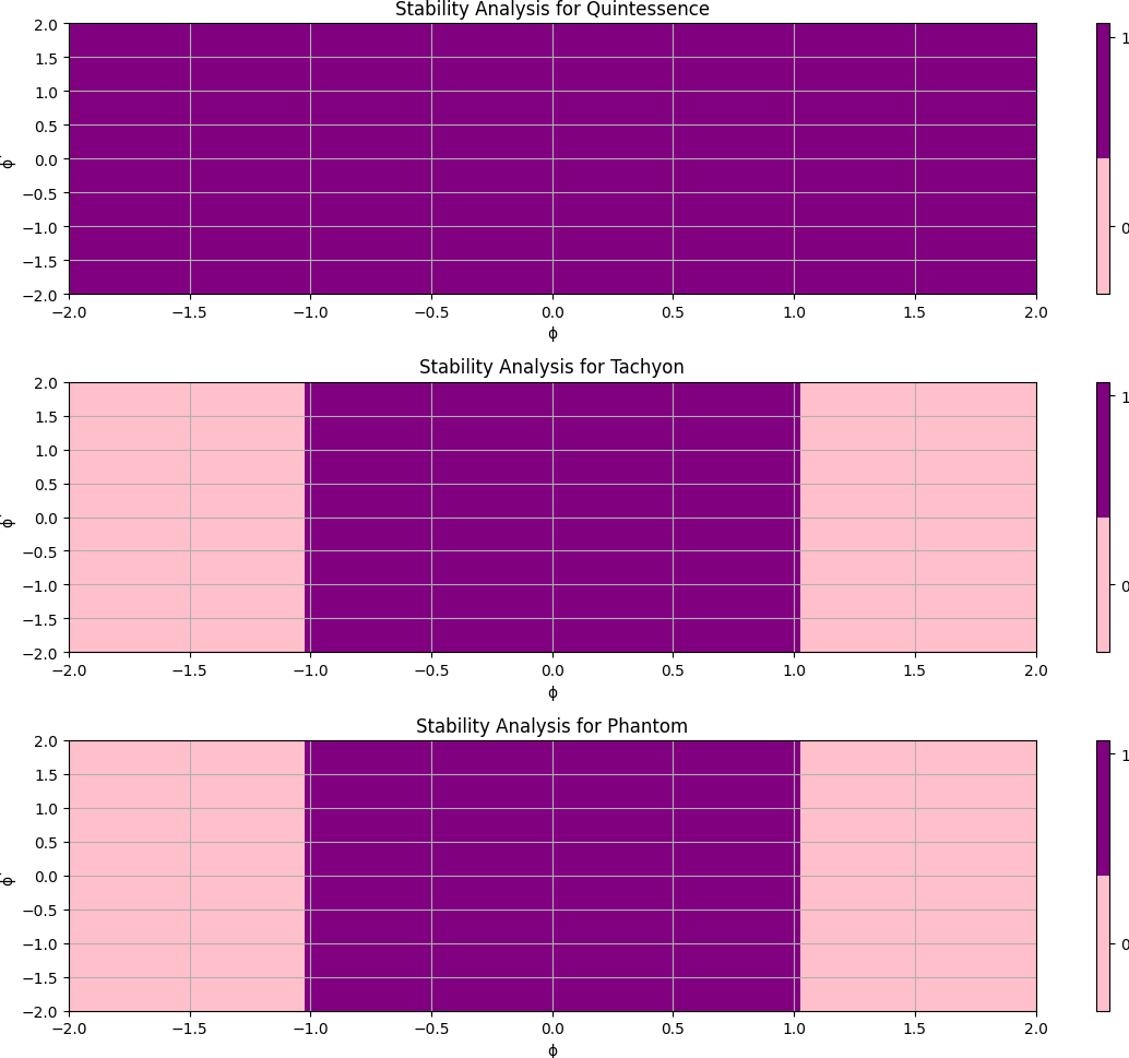
In this analysis, we varied the values of the scalar field $\phi$ and its time derivative $\dot{\phi}$ and identify stable regions based on the stability conditions discussed earlier. In Fig.1, three plots are plotted side-by-side, each representing the stability analysis for the quintessence, tachyon, and phantom fields with the same quadratic potential $V(\phi)=\frac{1}{2}m^{2}\phi^{2}$ . The plots provided a visual representation of the stable and unstable regions of the scalar fields in the $\phi-\dot{\phi}$ phase space. In the stable regions, the scalar fields evolve smoothly without encountering any instability or divergent behavior. On the other hand, in the unstable regions, the scalar fields may lead to unstable dynamics, and perturbations around their background solutions may result in instabilities. The plots show that each scalar field has a region of stability, which is essential for the viability of the corresponding cosmological models.

Now, we will analyze the stability of each case for different potentials.

Case 1: Quintessence field ( $\alpha=0$ )

Potential function:

V(\phi)=\frac{1}{2}m^{2}\phi^{2}

Equation of motion:

\ddot{\phi}+3\frac{\dot{a}}{a}\dot{\phi}+m^{2}\phi=0

The stability of the quintessence field can be determined by examining the mass term in the equation of motion, $m^{2}\phi$ . If $m^{2}>0$ , then the mass term will act as a stabilizing force, and the field will be stable around its minimum at $\phi=0$ . However, if $m^{2}<0$ , then the mass term becomes a destabilizing force, and the field will not be stable around $\phi=0$ . For the quintessence field to be stable, the mass parameter $m^{2}$ must be positive.

Case 2: Tachyon field ( $\alpha=-1$ )

Potential function:

V(\phi)=\lambda\phi^{4}

Equation of motion:

\ddot{\phi}(1-\dot{\phi}^{2})=3\frac{\dot{a}}{a}\dot{\phi}+\lambda\phi^{3}

In this case, the stability depends on the sign of the term $(1-\dot{\phi}^{2})$ in the equation of motion. If $(1-\dot{\phi}^{2})>0$ , then the tachyon field will be stable. However, if $(1-\dot{\phi}^{2})<0$ , then the field will be unstable. For the tachyon field to be stable, the quantity $(1-\dot{\phi}^{2})$ must be positive, which implies that $\dot{\phi}^{2}<1$ .

Case 3: Phantom field ( $\alpha=1$ )

Potential function:

V(\phi)=V_{0}e^{-\lambda\phi}

Equation of motion:

\ddot{\phi}(1-\dot{\phi}^{2})=3\frac{\dot{a}}{a}\dot{\phi}-\lambda V_{0}e^{-\lambda\phi}

Similar to the tachyon field, the stability of the phantom field depends on the sign of the term $(1-\dot{\phi}^{2})$ in the equation of motion. If $(1-\dot{\phi}^{2})>0$ , then the phantom field will be stable. However, if $(1-\dot{\phi}^{2})<0$ , then the field will be unstable. For the phantom field to be stable, the quantity $(1-\dot{\phi}^{2})$ must be positive, which implies that $\dot{\phi}^{2}<1$ .

In Fig.2, each plot shows the stability regions based on the stability conditions derived for each case. In the first plot, representing the quintessence field, the pink region corresponds to points in the $\phi-\dot{\phi}$ space where the stability condition is not satisfied, indicating instability. The purple region, on the other hand, represents stable points where both conditions (kinetic term and potential term) are met, ensuring a stable background for perturbations around the scalar field solution. The stable region covers most of the plot, indicating that the quintessence field is stable for a wide range of $\phi$ and $\dot{\phi}$ values. In the second plot, representing the tachyon field, the pink region denotes unstable points where the stability condition is violated. The purple region corresponds to stable points, indicating that the tachyon field is also stable for a significant portion of the $\phi-\dot{\phi}$ space. However, it’s important to note that the stable region is relatively smaller compared to the quintessence field, implying that certain regions of the tachyon field’s phase space may lead to instability. In the third plot, representing the phantom field, the pink region signifies unstable points where the stability condition is not satisfied. The purple region represents the stable region where both the kinetic term and potential term conditions are met, indicating a stable background for perturbations. Similar to the tachyon field, the stable region for the phantom field is smaller compared to the quintessence field, suggesting that certain regions of the phantom field’s phase space may lead to instability.

The overall stability of the scalar fields is influenced by the chosen potential function, and the quadratic potential demonstrates favorable stability properties for each case.

4 Behavior Analysis

Analyzing the behavior of the scalar field involves examining how the field evolves and changes over time. This analysis is carried out by studying the equations of motion, which are derived from the Lagrangian describing the scalar field’s dynamics. Solving these equations either numerically or analytically provides valuable insights into the field’s behavior. In our specific case, we performed numerical simulations using Python. To do this, we employed two numerical integration techniques: the Euler method and the fourth-order Runge-Kutta method (RK4). These methods allowed us to solve the equations of motion and Friedmann equations, which govern the evolution of the scalar field under the influence of the quadratic potential. The Euler method is a straightforward numerical integration technique that approximates the solution by taking small time steps and updating the field’s values accordingly. However, the Euler method may suffer from accuracy issues, especially for highly non-linear or oscillatory systems. To improve the accuracy and stability of our simulations, we utilized the fourth-order Runge-Kutta method (RK4). This method is more accurate than the Euler method and provides better stability properties. It involves calculating several intermediate steps to obtain a weighted average of function evaluations, resulting in a more reliable numerical solution. By performing these numerical simulations, we gained valuable insights into the behavior and stability of the scalar fields. The simulation setup required specifying initial conditions, such as the values of the scalar field and its derivatives, at a given initial time. Additionally, we needed to define the parameters in the equations, such as the potential function, the coupling constant, and the metric components. Furthermore, we carefully selected appropriate time steps to ensure a balance between accuracy and computational efficiency. The time step is the interval between consecutive time points at which the equations are solved. It needs to be small enough to capture the dynamics accurately, but not too small to avoid unnecessary computational burden.

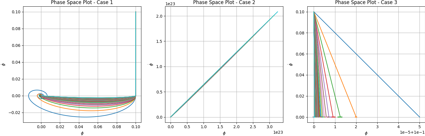
In Fig.3, the plots reveal distinct characteristics of the scalar fields’ evolution, and the trajectories showcase the dynamics of the scalar fields as they evolve over time. The quadratic potential and different field equations lead to distinct behaviors in the phase space, reflecting the dynamics and stability properties of the scalar fields under the influence of the given potentials. In Case 1, representing a Quintessence Field with $f(\alpha)=\frac{1}{2}$ and $\alpha=0$ , the phase space exhibits a single straight line followed by inward spirals that converge toward the origin $(0,0)$ . The straight line corresponds to a stationary scalar field, while the spirals represent the evolution of the scalar field toward the attractor at the origin. The system approaches stability over time, resulting in a stable Quintessence scenario. In Case 2, representing a Tachyon Field with $f(\alpha)=0$ and $\alpha=-1$ , the phase space reveals a distinct pattern of a straight line incorporating various trajectories in it. This behavior indicates that the Tachyon field evolves along a linear path towards a stable point, which represents the stability of the Tachyon scenario. In Case 3, representing a Phantom Field with $f(\alpha)=1$ and $\alpha=1$ , the phase space exhibits an intriguing behavior. The trajectories of the Phantom field appear to diverge away from the origin $(0,0)$ along different paths. However, it is essential to note that despite these outward trajectories, the stability of this scenario depends on the value of the equation of state parameter $w$ . For most values of $\phi$ and $\dot{\phi}$ , the Phantom Field is stable (satisfying $w>-1$ ), except for a critical point where $\alpha\cdot\dot{\phi}^{2}=1$ , which may lead to instability.

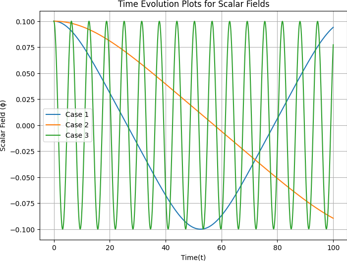
In Fig.4, we observe the time evolution of three distinct scalar fields, denoted by $\phi$ , depicted in different colors. Each scalar field follows a specific evolution pattern determined by its corresponding potential function $V(\phi)$ and the associated Hubble parameter $H(a)$ .

1. Case 1 ( $f(\alpha)=\frac{1}{2}$ and $\alpha=0$ ) : The scalar field $\phi$ evolves with a quadratic potential $V(\phi)=0.5\phi^{2}$ and a Hubble parameter $H(a)=\frac{1}{a}$ . The field exhibits harmonic oscillations around the potential minimum, remaining almost constant as the universe expands.

2. Case 2 ( $f(\alpha)=0$ and $\alpha=-1$ ): The scalar field $\phi$ evolves with a potential $V(\phi)=0.1\phi^{2}+0.05\phi^{3}$ and a Hubble parameter $H(a)=\frac{0.5}{a}$ . The field undergoes oscillatory behavior, with the oscillations damping as the universe expands.

3. Case 3 ( $f(\alpha)=1$ and $\alpha=1$ ): The scalar field $\phi$ evolves with a cosine potential $V(\phi)=\cos(\phi)$ and a Hubble parameter $H(a)=\sqrt{0.1+\frac{0.1}{a^{3}}}$ . The field exhibits periodic oscillations as the universe expands. The time evolution of each scalar field is influenced by the specific form of its potential function and the expansion rate of the universe characterized by the corresponding Hubble parameter.

Fig.5, shows the time evolution of the potential $V(\phi)$ for three different cases of scalar fields. Each case corresponds to a different potential function, and we will analyze them one by one.

1. Case 1 (Blue Curve - $V(\phi)=\frac{1}{2}m^{2}\phi^{2}$ ): The potential $V(\phi)$ is quadratic with a mass parameter $m=1.0$ . As time evolves, the potential $V(\phi)$ gradually increases. This behavior is typical of a scalar field with a quadratic potential. The scalar field $\phi$ evolves in a way that the potential energy increases, leading to a slow-rolling behavior. This is a characteristic feature of a scalar field known as ”inflation.”

2. Case 2 (Orange Curve - $V(\phi)=\lambda\phi^{4}$ ): The potential $V(\phi)$ is quartic with a coupling parameter $\lambda=1.0$ . Unlike the quadratic potential, the quartic potential increases more rapidly with time. As the scalar field $\phi$ evolves, the potential energy increases at a higher rate compared to Case 1.

3. Case 3 (Green Curve - $V(\phi)=V_{0}e^{-\lambda\phi}$ ): The potential $V(\phi)$ has an exponential form with a potential amplitude $V_{0}=1.0$ and an exponential parameter $\lambda=1.0$ . In this case, the potential energy gradually decreases with time as the scalar field $\phi$ evolves. The exponential potential leads to a behavior known as ”exponential expansion,” which can be associated with the late-time accelerated expansion of the universe (dark energy).

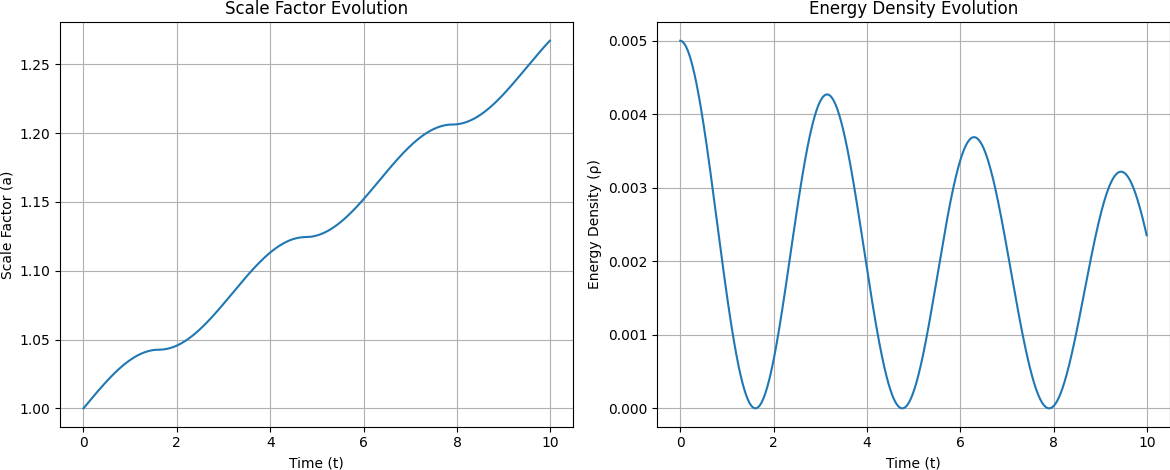
Fig.6, shows the evolution of the scale factor $(a)$ and the energy density $(\rho)$ of the scalar field over time.

1. Evolution of the Scale Factor (Left plot): The scale factor (a) represents the size of the universe at different times. As time progresses, the scale factor changes, indicating the expansion or contraction of the universe. In the plot, we observe that the scale factor increases with time, which suggests an expanding universe. This behavior is consistent with the standard cosmological model and the assumption of cosmic expansion.

2. Evolution of the Energy Density (Right plot): The energy density $(\rho)$ of the scalar field includes both the kinetic energy and potential energy associated with the field. In the plot, we observe that the energy density initially decreases as the universe expands. This is due to the dilution of energy as space expands, causing the energy density to decrease. As time progresses, the energy density of the scalar field reaches a minimum value and then starts to increase. This behavior indicates that the scalar field evolves and transfers energy from the potential to kinetic form, causing the energy density to rise.

Fig.7, shows the evolution of the scale factor and energy density in a cosmological scenario where a scalar field with a quadratic potential $V(\phi)=\frac{1}{2}m^{2}\phi^{2}$ is considered. The scalar field interacts with gravity and influences the dynamics of the expanding universe.

Initially, the scale factor starts at $a=1$ (normalized to unity) at $t=0$ , representing the present time or the initial condition of the universe. As time progresses, the scale factor increases rapidly, indicating that the universe is undergoing inflationary expansion. The inflationary period is characterized by an accelerating growth of the scale factor, which results in a significant increase in the size of the universe.

Also, initially, the energy density is relatively high but gradually decreases with time. The decrease in energy density is a consequence of the scalar field’s potential energy contribution ( $V(\phi)=\frac{1}{2}m^{2}\phi^{2}$ ) dominating over the kinetic energy contribution ( $\frac{1}{2}\dot{\phi}^{2}$ ) of the scalar field. As the scalar field evolves, its potential energy decreases, leading to a gradual decrease in the total energy density of the universe. The oscillations or fluctuations in the energy density are likely caused by the interplay between the kinetic and potential energy terms in the scalar field’s dynamics, leading to small variations in the rate of change of the energy density.

In Fig.8, the scale factor represents the size of the universe, and the plot demonstrates how it changes over time. Initially, the scale factor remains nearly constant, indicating a period of slow expansion or contraction. As time progresses, the scale factor starts to grow rapidly, indicating an accelerated expansion phase. The energy density of the field is a measure of its total energy, including both kinetic and potential energy contributions. At the beginning of the evolution, the energy density is high and then decreases gradually and becomes constant. The evolution of the scalar field in an expanding universe involves a gradual decrease in kinetic energy as the field velocity decreases due to the expansion’s damping effect. This decrease in kinetic energy is accompanied by an increase in potential energy as the scalar field approaches its equilibrium position. Eventually, the field settles into its equilibrium state, leading to a nearly constant energy density dominated by the potential energy of the scalar field.

5 Results and Discussion

The presented study introduces a unified Lagrangian that effectively captures the dynamics of tachyon, quintessence, and phantom scalar fields in diverse cosmological scenarios. Through numerical simulations and analytical calculations, the research offers valuable insights into the behavior of scalar fields under different potential functions and equations of state, contributing to a deeper understanding of cosmological evolution.

The emergent phenomena observed, namely inflationary behavior and late-time accelerated expansion, demonstrate the remarkable accuracy and versatility of the unified model in describing the cosmological dynamics of scalar fields. Inflationary behavior, observed in Case 1 with a quadratic potential, provides a compelling explanation for the large-scale homogeneity, isotropy, and flatness of the universe. On the other hand, late-time accelerated expansion, observed in Case 3 with an exponential potential, sheds light on the mysterious dark energy driving the universe’s current accelerated expansion.

6 Conclusion

This paper makes a significant contribution to theoretical physics and cosmology through the introduction of an innovative unified Lagrangian density. This Lagrangian effectively encompasses the behaviors of tachyon, quintessence, and phantom scalar fields by incorporating the function $f(\alpha)$ to account for different scenarios. The inclusion of the potential function $V(\phi)$ within this formulation further refines its accuracy in capturing the unique properties of these scalar fields. The study employs Python-based numerical simulations to comprehensively explore the dynamics of these scalar fields for varying $\alpha$ values. This approach allows for a thorough examination of their cosmological behavior. The numerical simulations yield valuable insights into the universe’s evolution guided by the unified Lagrangian, elucidating the specific features and implications of tachyon, quintessence, and phantom scalar fields within a cosmological context. A key finding is the successful application of this unified Lagrangian in describing the cosmological dynamics of these distinct scalar fields. The outcomes from numerical simulations showcase the remarkable fidelity of the unified Lagrangian in replicating observed cosmological phenomena linked to each scalar field scenario. This unification strategy introduces a more elegant and all-encompassing framework for comprehending scalar field behavior in the context of cosmology.

References

[1] Hubble, E.P., “A Relation between Distance and Radial Velocity among Extra-Galactic Nebulae”, Proc. Natl. Acad. Sci. USA, 15, 168–173 (1929).
[2] S. Perlmutter et al., Astrophys. J. 517, 565 (1999).
[3] A. G. Riess et al., Astron. J. 116, 1009 (1998); Astron. J. 117, 707 (1999).
[4] Aghanim, N., Akrami, Y., Ashdown, M., Aumont, J., Baccigalupi, C., Ballardini, M., … & Roudier, G. (2020). Planck 2018 results-VI. Cosmological parameters. Astronomy & Astrophysics, 641, A6.
[5] C. Wetterich, Nucl. Phys. B 302, 668 (1988).
[6] P.J.E. Peebles and B. Ratra, ApJ 325, L17 (1988).
[7] R.R. Caldwell, R. Dave and P.J. Steinhardt, Phys. Rev. Lett. 80, 1582 (1998).
[8] Y. Fujii, Phys. Rev. D 26, 2580 (1982).
[9] L. H. Ford, Phys. Rev. D 35, 2339 (1987).
[10] Y. Fujii and T. Nishioka, Phys. Rev. D 42, 361 (1990).
[11] T. Chiba, N. Sugiyama and T. Nakamura, Mon. Not. Roy. Astron. Soc. 289, L5(1997).
[12] S. M. Carroll, Phys. Rev. Lett. 81, 3067 (1998).
[13] R. R. Caldwell, Phys. Lett. B 545, 23-29 (2002).
[14] T. Padmanabhan, Phys. Rev. D 66, 021301 (2002).
[15] T. Padmanabhan and T. R. Choudhury, Phys. Rev. D 66, 081301 (2002).
[16] A. Sen, JHEP 9910, 008 (1999); JHEP 0204, 048 (2002).
[17] M. R. Garousi, Nucl. Phys. B584, 284 (2000); Nucl. Phys. B 647, 117 (2002).
[18] V. Sahni, T. D. Saini, A. A. Starobinsky and U. Alam, JETP Lett. 77, 201 (2003) [Pisma Zh. Eksp. Teor. Fiz.77, 249 (2003)].
[19] A. R. Liddle and D. H. Lyth, Cosmological inflation and large-scale structure, Cambridge University Press (2000).
[20] S. Weinberg, Gravitation and Cosmology, John Wiley and Sons, Inc. (1972).
[21] E. W. Kolb and M. Turner, The Early Universe, Addison-Wesley (1990).
[22] T. Padmanabhan, Theoretical Astrophysics, Cambridge Univ. Press (2000).
[23] Robertson, H.P. Kinematics and World-Structure. Astrophys. J. 1935, 82, 284–301.
[24] Robertson, H.P. Kinematics and World-Structure III. Astrophys. J. 1936, 83, 257–271.
[25] Walker, A.G. On Milne’s theory of world-structure. Proc. Lond. Math. Soc. 1936, s2-42, 90–127.
[26] Clarkson, C.; Basset, B.; Lu, T.H.-C. A general test of the Copernican principle Phys. Rev. Lett. 2008, 101, 011301.
[27] Zhang, P.; Stebbins, A. Confirmation of the Copernican principle through the anisotropic kinetic Sunyaev Zel’dovich effect. Phil. Trans. R. Soc. A 2011, 369, 5138–5145.
[28] Bentivegna, E.; Bruni, M. Effects of Nonlinear Inhomogeneity on the Cosmic Expansion with Numerical Relativity. Phys. Rev. Lett. 2016, 116, 251302.
[29] Saadeh, D.; Feeney, S.M.; Pontzen, A.; Peiris, H.V.; McEwen, J.D. How Isotropic is the Universe? Phys. Rev. Lett. 2016, 117, 131302.