Change Point Detection with Conceptors
Abstract
Offline change point detection retrospectively locates change points in a time series. Many nonparametric methods that target i.i.d. mean and variance changes fail in the presence of nonlinear temporal dependence, and model based methods require a known, rigid structure. For the at most one change point problem, we propose use of a conceptor matrix to learn the characteristic dynamics of a baseline training window with arbitrary dependence structure. The associated echo state network acts as a featurizer of the data, and change points are identified from the nature of the interactions between the features and their relationship to the baseline state. This model agnostic method can suggest potential locations of interest that warrant further study. We prove that, under mild assumptions, the method provides a consistent estimate of the true change point, and quantile estimates are produced via a moving block bootstrap of the original data. The method is evaluated with clustering metrics and Type 1 error control on simulated data, and applied to publicly available neural data from rats experiencing bouts of non-REM sleep prior to exploration of a radial maze. With sufficient spacing, the framework provides a simple extension to the sparse, multiple change point problem.
Keywords: change point detection, time series, echo state network, recurrent neural network, nonlinear dependence
1.3
1 Introduction
The offline change point identification problem is widely discussed in the literature, and used in a broad range of domains like signal processing, human activity monitoring, and finance (Truong et al. 2020). For time series data with , the goal is to retroactively identify points where the distribution changes. Despite the vast amount of work in this field, most of it is focused on identifying mean and variance changes, and the challenge of change point detection in the presence of nonlinear dependence is unresolved. Model based methods assume a known, rigid structure, and specification of a functional form to fit nonlinearities present in data can be difficult. Many nonparametric methods are only applicable to independent and identically distributed data, and are applied to cases where changes would be easily identified from visual inspection of a time series plot. Unless they target the aforementioned mean and variance scenarios, most nonparametric methods also have an uninterpretable or shrouded definition of the notion of “change.” The contribution of this paper is a model agnostic method for detecting change in multivariate and arbitrarily dependent nonlinear time series data.
The conceptor change point (CCP) methodology builds on prevalent ideas in statistics and representation learning literature. High-dimensional featurizations from echo state networks (ESNs), and a conceptor matrix from a specified and interpretable “baseline” state, allows for the flexibility of change detection in processes with elaborate dependence structures. This methodology should be used as a tool to suggest potential locations of interest in a dataset where traditional methods and inspection fail.
For this work, the framework is restricted to the at most one change point (AMOC) problem. The distribution functions for each vector in time and are compared with the hypotheses
| (1) |
where and are unknown. Rejection of the null leads to the conclusion that a change took place immediately after time point . With sufficient spacing, the framework provides simple extensions to the sparse, multiple change point problem and the online, sequential change point problem.
1.1 Change Point Detection
Change point detection methods can broadly be classified as sequential, agglomerative, or divisive. Sequential change point detection, like that of Lai 1995, best lends itself to the online problem where changes are identified in sequence while the data is observed. Online change point detection is not the main focus of this manuscript. Agglomerative change point methods begin by labelling each data point as a unique cluster, and proceed by strategically grouping adjacent clusters with an algorithmic criterion; Fryzlewicz 2018 and Matteson and James 2014 provide two examples of these criteria.
Divisive algorithms cluster a series of points and algorithmically search for breaks that best divide into chronological classifications. Many of these algorithms follow the binary segmentation approach, pioneered by Vostrikova 1981, and identify subsequent change points from each of the divided pieces. Penalized techniques like Ombao et al. 2005, Lavielle and Teyssiere 2006, and Killick et al. 2012 are also prevalent and recent computational work by Haynes et al. 2017 and Tickle et al. 2020 build on these methods and aim to optimize the search process for efficient change point detection. CUSUM type statistics provide the most common foundation to locate change points in ordered sequences (Picard 1985; Gombay and Horváth 1995; Gombay and Horváth 1999; Cho and Fryzlewicz 2012; Holmes and Kojadinovic 2021; Kojadinovic and Verdier 2021). Many modifications are in the form of the Kolmogorov-Smirnov and Cramer-von Mises criteria, including the self-normalization method of Shao and Zhang 2010. Most initial work in this field, like wild binary segmentation of Fryzlewicz 2014, applies only to univariate sequences, and several extensions of these methods to multivariate and high-dimensional applications build on the respective univariate versions (Cho and Fryzlewicz 2015). Matteson and James 2014 propose a clustering algorithm based on a hierarchical divergence measure for the multivariate, multiple change point problem. This method imposes the strict assumption of independent and identically distributed data and is only asymptotically justified in the AMOC problem (Arlot et al. 2019). Projection of the data into a high-dimensional space by Wang and Samworth 2018, the kernel trick for change point estimation by Arlot et al. 2019, and Bayesian estimation like Cappello et al. 2023 also import the assumption of independent data. Dehling et al. 2015 and Dehling et al. 2022 investigate relaxing the i.i.d. requirement by examining the effect of short-term dependence on large sample behavior, and Gerstenberger 2018 explores only the mean change problem for short-term dependence. Certain types of model based detection like Kirch et al. 2015 also relax the i.i.d. requirement, but rely on strong parametric assumptions and impose a rigid structure onto the process. Characterizing nonlinear temporal dependence in change point problems is a challenging, relevant problem with relatively little progress.
1.2 Conceptors
An ESN expands an input sequence to a nonlinear, high-dimensional feature space that captures distinct characteristics of the data via a fixed, sparsely connected reservoir of randomly intialized weights. The universal approximation theorems of Cybenko 1989 and Hornik 1991 have been extended to recurrent neural networks (RNNs) and ESNs with a sufficient reservoir size, and features that are not linearly separable in the original input space can become separable in the reservoir (Lukoševičius 2012; Grigoryeva and Ortega 2018; Hart et al. 2020; Gonon and Ortega 2021). The reservoir is composed of randomly populated matrices, , , and in Equation 2, and the output sequence is obtained from a simple linear mapping () of the feature space, usually trained with Ridge regression (Jaeger 2002; Jaeger 2007).
Jaeger 2014 introduced the conceptor as a regularized identity mapping of reservoir states in a propagating ESN. A matrix is added to the update equation that recognize, control, regenerate, and predict state patterns in a dynamic reservoir (Jaeger 2014; Jaeger 2017). The matrix is placed at the front of Equation 3 to filter the network states in a manner associated with a specific pattern.
| (2) | ||||
| (3) | ||||
| (4) |
The conceptor matrix , defined in Equation 5, is computed from column space of the reservoir states over some training window of data (of integer length ) that exhibits a pattern of interest. For dynamics associated with the pattern from the training window, the conceptor matrix should leave the state unchanged and act like the identity, or (Jaeger 2017). For states propagating in a fashion atypical for the pattern from the training window, the conceptor matrix will act like the null matrix and suppress the reservoir state (Jaeger 2017).
Over the training window, compiles the reservoir states as individual rows (where prior to computation in the training window). The conceptor is a positive semidefinite matrix () that forms an ellipsoid within the unit sphere. The principal axes of the ellipsoid are the eigenvectors of the reservoir state second moment matrix that have been scaled by their eigenvalues.
| (5) |
A regularization parameter , known as the aperture, influences the degree of dampening in the reservoir activity (Jaeger 2014; Jaeger 2017). Large apertures introduce small penalties, and the conceptor will tend to the identity with minimal activity dampening; smaller shrinks the conceptor to the zero matrix.
In many applications, conceptors are appealing for prediction and pattern regeneration tasks because it is possible to remove the input data from the update equation. Equation 2 is modified to , where is trained from the input and reservoir states, and the conceptor governs the dynamics of the system autonomously (Jaeger 2014; Jaeger 2017).
In this work, conceptors are used to encapsulate the dynamics of a training window of data. The ESN featurization serves as an advantageous functional transformation to a high-dimensional domain where nonlinear relationships are “linearized” without imposing a rigid structure. A specified training window serves as an interpretable baseline state, the conceptor records information about the baseline dynamics, and the relationship between the reservoir states and filtered states is used to highlight differences in the mechanism of evolution.
Nonlinear temporal dependence is difficult to characterize, especially in multivariate time series. Linear tools often oversimplify the dependence structure, and choosing a “close enough” functional form can be a challenging task. The CCP methodology allows for flexible change point detection in processes with elaborate dependence structures.
2 Methodology
The hypothesis in Equation 1 is tested under the condition where at most one change point is present in the data. The selected training window should be sufficiently long to capture the original dynamics of the time series and include representative values from the data prior to a suspected change. If the data exhibits a periodic or almost-periodic type structure, the training length should include at least one full cycle. It is assumed that any change takes place after this baseline window, and the initial distribution produces a time series that is at least wide-sense cyclostationary. The second assumption ensures the training data covers a relevant range of the data and changes are not falsely identified from unrecognized network dynamics. The training window need not be at the beginning of the time series; this can be generalized to take any section as a baseline state, where the method looks forward and backward for a potential change.
The proposed method involves three main steps. First, several ESNs are generated and the specified training window is used to select network parameters that satisfy an error tolerance , defined in terms of the normalized root mean square error (NRMSE) of the reservoir output, . For each ESN, a conceptor matrix is computed that encodes information about the dynamics of the training window of a time series. Second, the relative differences between the reservoir and filtered states are examined with a bisection technique that proposes a change point. Last, a moving block bootstrap is used to estimate the strength of evidence for a proposed change.
2.1 ESN Featurization
Along with an integer length for the baseline , an integer length is specified and used to washout the initial conditions of a generated ESN reservoir, where generally . A training error influences hyperparameter settings; this error tolerance is the maximum allowable NRMSE between the conceptor governed ESN output and the original data. Define , and the assumption of no distributional change applies to the time points where , restricting the identification of any change point to the interval .
A reservoir size is selected where . A series of ESNs are initialized by generating the matrices from Equation 2. The input and bias matrices, and , are dense with independent random Gaussian realizations, where the variance is determined from a parameter grid such that the ESN output best fits the data as measured by NRMSE. Each is a sparse matrix with independent random Gaussian nonzero entries, and is scaled to a constant spectral radius of 0.8 to ensure the propagating reservoir states remain stable and wash out (or “forget”) the information from any initial conditions. The chosen spectral radius is not at the limit of stability as a balance between introducing adequate temporal dependence and ensuring the reservoir washout does not waste valuable data (Lukoševičius 2012; Yildiz et al. 2012).
The reservoir size and aperture of the network are concurrently determined as the first values large enough to produce a NRMSE below . Selection of should take place prior to analysis and not with iterations of the method on multiple parameter values. Smaller values may be more sensitive to learning variations in the noise component of the data, while larger values will extract general behavior. In Section 4, the effect of varying is demonstrated, but the parameter should take a default of about 4 to 8% NRMSE unless compelling prior knowledge about the type of change sought suggests otherwise. Parameter selection procedures and the full ESN featurization algorithm are given in the supplement.
For each ESN featurization, the associated conceptor matrix is computed from the series of training time points after network washout, . The network is propagated forward in time via Equations 2 and 3 with , and the reservoir states () collected. Conceptor matrices are obtained via Equation 5; then, each ESN is run with in place, like Equation 3, for all time points .
2.2 Change Point Proposal
The angles between the filtered states and the reservoir states are examined at each time after the training period. The cosine similarities of these angles , for each featurization , form univariate sequences that quantify the proximity of the reservoir states to the space spanned by the corresponding conceptor matrix.
| (6) |
Values in each sequence are contained in the interval because, by definition, each is positive semidefinite. A similarity value can be interpreted as a measure of the strength of relationship between the reservoir state at time and those in the period of training data. Values of zero imply the ESN is generating states orthogonal to the conceptor space, and those equal to one imply the ESN is generating states exactly in the conceptor space.
Other distance measurements may be used to quantify proximity to the conceptor space. Cosine similarity is a bounded, interpretable quantity that emphasizes angles further from zero at an increasing rate. The exact values of these similarities will vary and their absolute measure is not important; only relative differences are needed for comparison throughout the time series. Figure 7 and others in the supplement illustrate the relative nature of the similarity measure.
Because the networks are randomly generated, there is variation in the computed conceptor matrices that extends to the cosine similarities across the ESNs. To extract a general behavior and reduce the dimension of the information, the average cosine similarity at each time point is considered, . The aggregate cosine similarity sequence acts as an ensemble of weak learners from each generated ESN.
A proposed change point is selected using a modified CUSUM statistic that resembles the two-sample Kolmogorov-Smirnov distributional test (Smirnov 1933). From the sequence , empirical CDFs and are constructed by dividing the sample at each potential change point in the series.
| (7) | ||||
| (8) |
A scaled statistic, like that used in Gombay and Horváth 1995 and Padilla et al. 2019, is computed at each observation, and the point of the maximum is identified as the most likely change point:
| (9) | ||||
| (10) |
The coefficient term in Equation 9 ensures the statistic converges in distribution under stationarity as (Csörgő and Horváth 1997; Gombay and Horváth 1999; Holmes et al. 2013; Kojadinovic and Verdier 2021). The scaling function, with form shown in Equation 11, increases the sensitivity of the method near the edges of the sequence (Csörgő and Szyszkowicz 1994a; Csörgő and Szyszkowicz 1994b; Csörgő and Horváth 1997; Csörgő et al. 1997). Further properties of the statistic under the null are discussed in Section 3.
| (11) |
The statistic given in Equation 9 is similar to that discussed in Kojadinovic and Verdier 2021, where if and is a small constant near zero, the mean and variance of the series of statistics remain approximately constant in the limit. Values and are chosen for reasons explained in Section 3, and the full algorithmic process for proposing a change point is detailed in the supplement.
2.3 Moving Block Bootstrap
Estimating the null distribution of the statistic from Section 2.2 may be of more importance than the identification of a potential change point. By nature, many change point detection problems are non-verifiable in real world applications. Thus, reliable change point algorithms should be robust in their ability to detect both change and the lack of change in a dataset.
The bootstrap method of Efron 1979 provides a foundation for inference based on repeated sampling. Several variations of the bootstrap for change point methodology are reviewed in Hušková 2004. The moving block bootstrap (MBB), developed by Kunsch 1989 and Liu and Singh 1992, samples blocks of consecutive points to retain the dependence structure within each block. Extending the bootstrap to applications with dependent data structures, the MBB is able to asymptotically reproduce the underlying dependence structure (Lahiri 2003). The block bootstrap is suggested by Dehling and Philipp 2002 for statistics of empirical processes, and Synowiecki 2007 describes its application to non-stationary data with periodic or almost periodic behavior.
Potentially overlapping blocks of length are selected and combined to form a bootstrapped time series of the original length . When data are treated as i.i.d., as in Matteson and James 2014, the block length parameter reduces to a permutation of the time series with . With increasing block length, the estimated null distribution will exhibit less variation, and null values will tend closer to the statistic . Choice of block length is discussed widely in literature, and the cross-validation like technique of Hall et al. 1995 allows for data driven selection (Bühlmann and Künsch 1999; Lahiri 2003; Politis and White 2004; Lahiri et al. 2007; Patton et al. 2009). A large pilot block length is used to start the Hall et al. 1995 algorithm to ensure a long range dependence structure is considered, and the process is not iterated as convergence is not guaranteed (Lahiri 2003). Adjusting the block length for the power and Type 1 error control trade-off should be considered if the researcher possesses some knowledge about the dependence structure of the data.
With the assumption of no change in the washout and training windows, the conceptor matrices do not need to be recomputed: in each bootstrapped series the points are identical to the original data. All remaining points are equally likely to be chosen as the beginning of a bootstrap interval of length . To ensure equal inclusion probability, the series is wrapped such that a block near the end (a time point within of ) will cycle back to the initial time considered, .
For each generated bootstrap time series , the corresponding maximum statistic is computed as in Section 2.2, simulating an approximate null distribution. A distribution quantile is estimated from the fraction of the bootstrapped statistics that exceed the statistic from Equation 9, . The quantile estimate provides a notion of the strength of the evidence for a change point. The validity of applying the MBB to the AMOC problem is investigated through simulation and evaluation of Type 1 error control in Section 4 for a variety of data generating processes. For a dataset with no change point, the proportion of false rejections in simulations is expected to be approximately , where is a predefined threshold of Type 1 error. The full algorithm for estimating a null distribution from the MBB is in the supplement.
3 Theory
The hypothesis in Equation 1 is tested using the featurization and conceptor matrix as outlined in Section 2. Under the null hypothesis, the cosine similarity values are expected to retain a consistent relative structure and fall close to one (i.e., remain close to the space of the conceptor matrix). Under the alternative, changes in the relationship between the cosine similarity sequence and the space spanned by the conceptor matrix are observed. These changes, initiated by a shift in the data, are not strictly away from the conceptor space; a reduction in variation may lead to reservoir states that lie closer to the conceptor space.
For clarity, the time index is redefined to and as the number of data points after washout and training. The assumption of any change after washout and training restricts the domain to . Suppose for all , where each is a defined distribution function. The hypothesis is reformulated in terms of these distribution functions.
| (12) |
Define the corresponding empirical distribution functions at each point in the time series , and . By the Glivenko-Cantelli theorem, these empirical CDFs are consistent estimators of the true distribution functions and they uniformly converge in the limit under stationarity and ergodicity (Tucker 1959; Yu 1993; Dehling and Philipp 2002). Summarizing the data with the univariate sequence generated by the conceptor space , rather than using the original multivariate time series, may also make investigation and verification of theoretical assumptions more accessible.
3.1 Limiting Distribution Under the Null Hypothesis
Asymptotic behavior of empirical processes for i.i.d. sequences stems from Kiefer 1972, that proved almost sure convergence to a Gaussian process. In this work, the -mixing definition of Berkes et al. 2009 is used to obtain a similar result for the statistic in Equation 9.
Assume the sequence is stationary under the null hypothesis, satisfied by construction in Equation 12, and can be represented as a shift process of i.i.d. random variables , . Most stationary processes in practice admit a representation as a shift process, and this is causal due to the forward dynamics of the time series (Berkes et al. 2009). These assumptions apply only to the sequence indicating the relationship of a given state to the baseline space spanned by the conceptor matrix; they are not imposed on the original data. In a time window without a change point present, assume will arise from some common distribution. A process as -mixing if the two conditions in Definition 3.1 are satisfied.
Definition 3.1.
A random process is -mixing if:
- (1)
For any and , one can find a random variable such that
for some numerical sequences , . - (2)
For any disjoint intervals of integers and any positive integers
, the vectors are independent
provided the separation between and is greater than .
With mild assumptions on the function , Berkes et al. 2009 easily show the shift process representation for a general class of nonlinear processes. Construction of the approximating sequence is discussed via substitution, truncation, coupling, and smoothing techniques (Berkes et al. 2009). -mixing is not directly comparable to classical mixing conditions, like -, -, or -mixing. The classical mixing definitions lead to clean and precise theoretical results, but verifying the required conditions can be challenging and their scope of application is limited (Berkes et al. 2009). -mixing relaxes these requirements to the existence of an approximating sequence that satisfies the above properties. Within the targeted class of shift processes, verification of assumptions is almost immediate, and the resulting strong approximation is used to derive the limiting distribution (Berkes et al. 2009).
Define the function by and some small resembling Equation 11 with .
Theorem 3.2.
Let be a stationary sequence such that is Lipschitz continuous of order . Assume is -mixing and that condition (1) of Definition 3.1 holds with , for some . Under the null hypothesis for every ,
| (13) |
as , where is a Gaussian process with
| and | (14) |
and the limiting random variable is almost surely finite.
The mathematical exposition and proof is an extension of the independent case found in Csörgő and Horváth 1997, Theorem 2.6.1 and can be found in the supplement. Theorem 3.2 implies the statistic converges in probability to zero under the null hypothesis.
Stationarity of the average cosine similarities depends on the training window of data and adherence to the AMOC problem. With a well specified, sufficiently long training window such that a relevant range of the time series is covered, the reservoir will emit dynamics close to the conceptor space and the assumption is likely satisfied. With multiple changes present in a dataset, the stationarity assumption may be violated. In practice, the data should be at least wide-sense cyclostationary, contain at most one change, and not exhibit some long run trend.
3.2 Consistent Change Point Estimation
The behavior of the change point estimate is examined under the general class of alternatives given in the hypothesis of Equation 12. Under construction of the alternative, the average cosine similarity sequence divides into two stationary ergodic pieces on either side of a true change point represented by and . When satisfying modest conditions, is a consistent estimator of .
Theorem 3.3.
Suppose the sequence , divides into two stationary ergodic pieces on either side of the change point , and for some . Then for every , the change point estimate
| (15) |
converges in probability to the true value under the domain restriction
| (16) |
The proof in the supplement follows Theorem 2.1 from Newey and McFadden 1994 for consistency of extremeum estimators. Restricting a possible change point to the interval shown in Theorem 3.3 does not shrink the domain in practice if the chosen .
4 Simulation Study
Performance of the CCP method is demonstrated through simulations restricted to the AMOC problem. The CCP method is compared to the e-divisive (EDiv) method of Matteson and
James 2014 and the kernel change point (KCP) algorithm of Arlot
et al. 2019, both via the ecp R package by James and
Matteson 2015, along with the sparsified binary segmentation (SBS) methods of Cho and
Fryzlewicz 2015, via the sbs R package by the same authors. Type 1 sparsified binary segmentation searches for changes in the center of the data, and Type 2 seeks other forms of distributional change (Cho and
Fryzlewicz 2015).
4.1 Simulation Settings
Simulated time series fall into the broad classes of VAR, periodic, Gaussian, and white noise processes. All simulated data , , has length with a potential change located from to . Table 1 summarizes the settings used for each method in the study. CCP requires specification of a training length of data with an associated training error tolerance.
| Method | Settings |
| Conceptor Change Point (CCP) | |
| E-Divisive (EDiv) | |
| Kernel Change Point (KCP) | , |
| Sparsified Binary Segmentation (SBS) | , |
The washout length and the training length are fixed to ensure a constant window of estimation for all compared methods. The error tolerance varies from 2 to 16 percent of NRMSE. The EDiv, KCP, and SBS methods are restricted to the AMOC framework. For EDiv and SBS the estimate is the initial segmentation chosen by the algorithm. KCP accepts an input parameter to restrict to the AMOC problem. EDiv, SBS1, and SBS2 require a significance threshold for change point identification that is set to . The same value is used in the CCP method to set an upper threshold on the bootstrap null distribution. KCP requires specification of a penalty parameter for change point identification; Arlot et al. 2019 outline a procedure for selection of this parameter, and the suggested penalty scaling is used.
When a change in the data is present, the adjusted Rand index (ARI) of Hubert and Arabie 1985 compares the assignment of time points to the correct class, and the empirical CDF of the difference between the identified point and the true change point is computed. Given in Equation 17, with the fraction of the time series away from the true change point and the total number of simulations for a selected setting, the empirical CDF shape in some neighborhood compares performance of the methods.
| (17) |
Better performing methods will quickly increase to 1, and those that fail to identify an existing change point are evaluated as if it was placed at the end of the series, . When no change is present, is defined as the observed Type 1 error and compared with the defined threshold .
Tables 2 and 3 detail the datasets examined in the simulation study. For each case, a no change point scenario is included where the initial data generating process held constant for the full time series. Each setting is indicated by a unique ID and repeated times to create over simulated datasets.
| ID | Simulated Data | ID | Simulated Data | |
| (1a); (2a) | (3a) | |||
| (1b); (2b) | (3b) | |||
| (1c); (2c) | (3c) | |||
| (1d); (2d) | (3d) | |||
| (1e); (2e) | (3e) | |||
| (1f); (2f) |
| ID | Simulated Data | ID | Simulated Data | |
| (4a) | (5a) | |||
| (4b) | (5b) | |||
| (4c) | (5c) | |||
| (4d) | (5d) | |||
| (4e) | (5e) | |||
| (4f) | (5f) | |||
| (4g) | (5g) | |||
| (4h) | (5h) | |||
| (4i) | (5i) |
For VAR processes, the coefficient matrix is randomly generated to have a fixed spectral radius (within a tolerance of 0.02). Change points from autoregressive processes with similar may be more difficult to identify as they can exhibit similar dynamics. All VAR processes contain a white noise error term defined in Table 2. For periodic processes, the second dimension is shifted by of as noted by the braced parenthesis in Table 2, and all contain a white noise error term. The Ornstein-Uhlenbeck processes are defined by the stochastic differential equation , where denotes a two-dimensional Wiener process. The two-dimensional Ornstein-Uhlenbeck process is denoted , where is the mean-reverting matrix and is the volatility matrix. Gaussian white noise processes with mean, variance, and covariance shifts are included in the simulation to compare CCP methodology to existing methods in benchmark scenarios.
4.2 Simulation Results
Simulation results and figures for dependent processes are presented in this section. Tables of results, and tables and figures for white noise processes included for comparison to existing methods, are given in the supplement.
For VAR() processes with a change point present, the CCP method outperforms existing methodology. This advantage increases with more lagged values in the dependence structure and when process transitions to a relatively large spectral radius. Figure 1 displays the graphical evaluation technique defined in Equation 17.
Among the conceptor methods, the higher error tolerances (CCP08 and CCP16) provide a more general fit to the data, where smaller error tolerances (CCP02) produce networks with larger reservoirs that learn the minor deviations of the data. In the presence of noise, these minor deviations occlude the true signal, potentially leading to inconsistencies in the learned behavior. Caution should be taken when specifying the error tolerance in noisy data; moderate tolerances may perform better than small tolerances as they fit networks with constrained internal dynamics, placing more emphasis on a general signal. This phenomenon can be likened to an overfitting problem. The KCP and SBS2 methods are the closest existing methods to the conceptor performance. One major drawback of the SBS method is that the type of change point sought must be specified; the algorithm run with a Type 1 designation produces very low ARI scores for all VAR() simulations.
Figure 2 shows the results for simulations where the underlying data is generated by a periodic process. The CCP method is able to reliably detect changes in the frequency of periodic processes when the deviation from an initial state is sufficiently large; existing methodology struggles with this class of processes. While methods in the frequency domain easily detect this type of change, methods that exist in the temporal domain often fail with periodic data. The CCP method in the temporal domain is able to capture this type of nonlinear dependence, as well as those more readily described by the time axis.
Figures 3 and 4 display results for Ornstein-Uhlenbeck simulations with a mean reverting or volatility parameter change. The CCP method surpasses most other methods for detection in mean reverting parameter changes except in some cases when the data shifts to a random walk process (or the parameter goes to zero). The difficulties for all methods can likely be attributed to a relatively low signal to noise ratio. For the volatility, the CCP method is competitive with existing methodology. This behavior is also seen in white noise variance simulations (see suplementary material) that play to the strengths of the comparator methods. With a high signal to noise ratio, the CCP method is also competitive in detecting mean changes in white noise processes.
To evaluate the validity of the moving block bootstrap in the CCP method, the Type 1 error of each method is observed when no change takes place in the time series. Control for false discovery of change points is as important as the correct identification of a change. Figure 5 shows the observed probability of erroneous detection for each method. SBS methods provide conservative error control, KCP methodology almost always flags a change point, and EDiv does not hold to a desired level for data that is not Gaussian white noise. SBS methods do not return a quantile estimate, but only a binary “present” or “not present” flag; to estimate coverage at the points indicated, the method was run with different values of the threshold . CCP methodology tracks along the uniform cdf with only slight undercoverage in periodic data and VAR data with large spectral radii.

5 Application Study
The CCP method is applied to data from Varela and Wilson 2019. The authors record local field potential (LFP) up to 600Hz in the midline thalamus (THAL), medial prefrontal cortex (PFC), and the CA1 region of the hippocampus (HC) in rats experiencing bouts of non-REM sleep and wakefulness while they remained in a quiet, square-shaped enclosure (Varela and Wilson 2019; Varela and Wilson 2020). The data, obtained from the Collaborative Research in Computational Neuroscience data sharing website, also includes determinations of sleep state (awake or non-REM sleep), as well as spiking, spindle, and sharp-wave ripple information over the course of the experiment (Varela and Wilson 2019). Session 1 is selected (prior to exploration of a radial maze), and the data is filtered with a finite impulse response filter to focus on the delta band (1-4Hz), characterizing slow wave sleep. Finally, the data is downsampled to a frequency of 4Hz.
Three periods of transition identified by Varela and Wilson 2019 are isolated; each spans 100 seconds: sleep to wake (650 to 750s, change point at 740s), wake to sleep (740 to 840s, change point at 800s), and wake to sleep (1080 to 1180s, change point at 1150s). Relatively short windows are selected to satisfy the AMOC assumption; shorter time periods focus the methods to detecting the sleep state transition rather than other dynamic neural process changes almost certainly present in the data. The CCP, EDiv, SBS2, and KCP methods are evaluated on their ability to locate the change points in each transition period.
Approximately 10 seconds are reserved for reservoir washout, and 30 seconds are used for conceptor training with the CCP method. Change points are identified in the remaining one minute for all methods. Settings for methods are given in Table 1, and the CCP error tolerance is kept at NRMSE. Figure 6 presents the results from applying the methods to the LFP data. Methods that fail to identify a change point display as a vertical line at the far right edge of the figure.
Figure 7 displays the internal dynamics of the conceptor methodology applied to the first (top) time series segment in Figure 6. Similar visuals of the second and third segments are shown in the supplement.
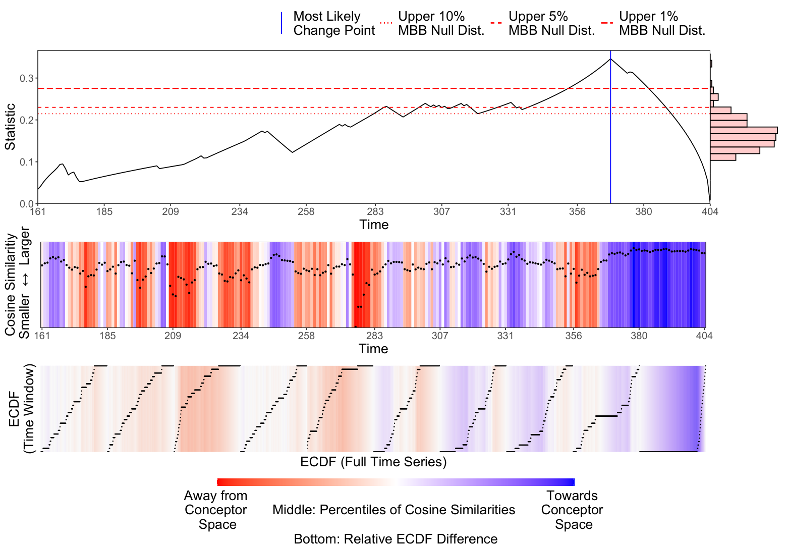
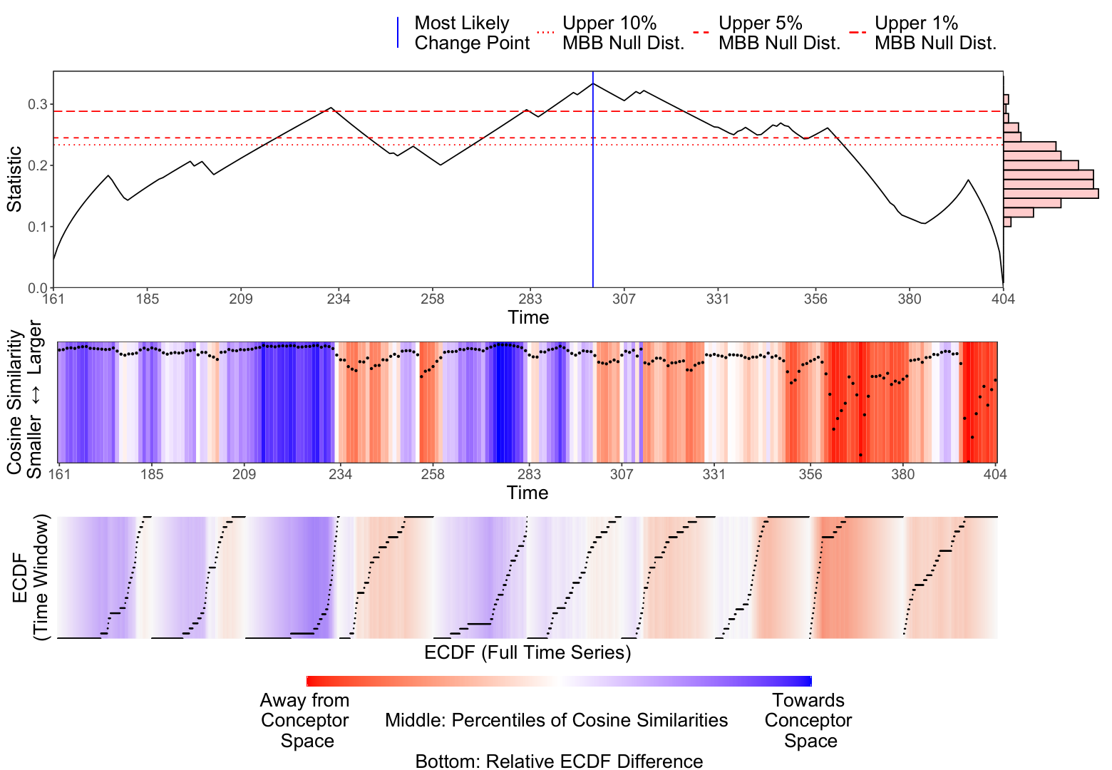
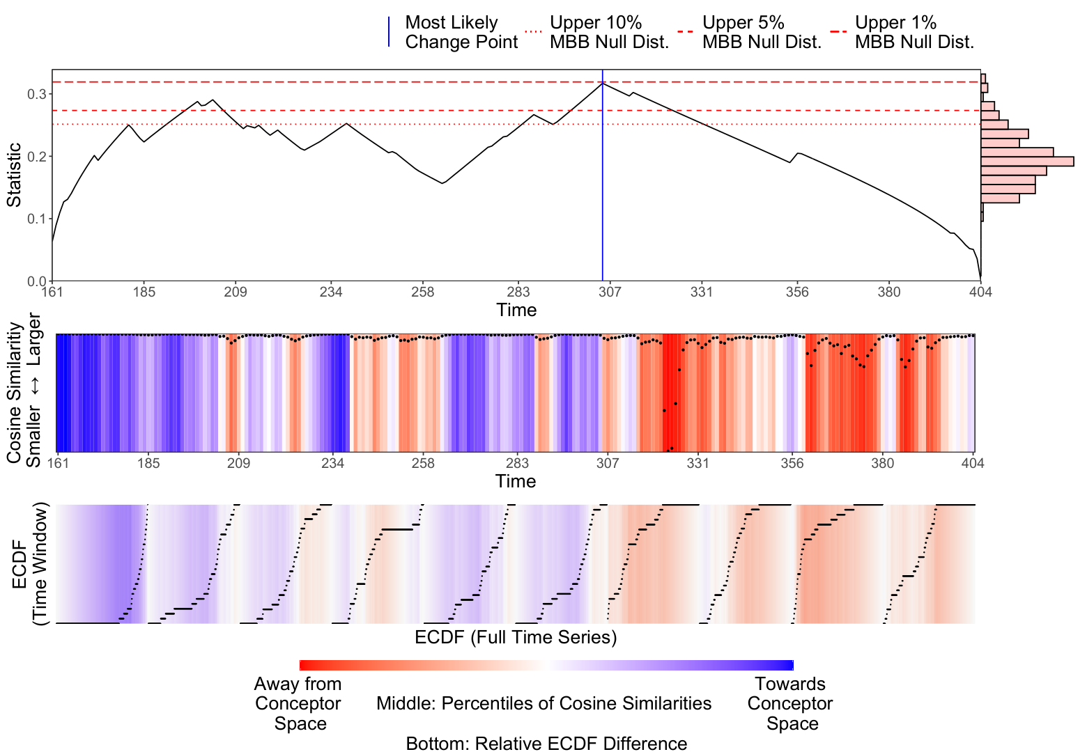
The top plot of Figure 7 displays the series of CUSUM-like statistics, with an estimated bootstrap null distribution on the right vertical axis and quantiles as horizontal lines on the plot. The middle plot displays with a relative vertical axis, as only comparative differences through the time series are sought. The bottom plot gives empirical CDFs of over segmented windows of time; the plotted points display the difference between the empirical CDF of the specific window and the overall empirical CDF of the full time series. Shading in the middle and bottom plots represents the internal reservoir dynamics and their relationship to the conceptor space; blue refers to dynamics that are behaving similarly to the original conceptor space, and red indicates further away. The scale of color shading in the middle plot is tied to percentiles the sequence , and in the bottom plot is a relative difference between empirical CDFs. Change points will be identified as a peak in the top plot and a color transition in the middle and bottom plots. Excessive undulation, a secondary peak, or multiple shifts may suggest violation of the AMOC assumption or a slow transition between states.
6 Discussion
The CCP method provides a model agnostic framework for addressing nonlinear temporal dependence in change point identification problems. This relaxes the common i.i.d. assumption of most existing methodology, and allows for flexible definition of a baseline state without the rigidity of an imposed structure. The method also alleviates the problem of specifying a functional nonlinear form, which can be challenging.
The ESN learns the characteristic dynamics of a training window, and the deviation from the conceptor space is examined with a CUSUM-like statistic that consistently estimates the true change point under mild assumptions. The method is able to flag important locations for future scrutiny and provide guidance on the strength of evidence for a change point via the moving block bootstrap. CCP outperforms existing methods in temporally dependent and periodic processes, and is even competitive in i.i.d. processes with a change in variation or a high signal to noise ratio. In practice, the training window should be sufficiently long to capture representative variation of the original time series, and left at a default value unless there is prior knowledge of the type of change sought. Assumptions include a baseline period of stable data generation where the data is at least wide-sense cyclostationary, and stationarity of the obtained similarity sequence on either side of at most one potential change point . Violation of the cosine similarity stationarity assumption will affect theoretical results, but does not diminish use of the method for investigative study of a dataset. Implementation of the method may require isolation of a time segment of interest, like the application in Section 5, so that the AMOC assumption is met. These segments must be identified by the researcher with prior knowledge of their data. This method provides straightforward extensions to the multiple change point problem, and to online, sequential detection provided changes are sparse and sufficiently spaced. Future work can improve the featurization process so that information pertaining to individual series in the data is preserved, making qualitative conclusions about change points more accessible.
References
- Arlot et al. (2019) Arlot, S., A. Celisse, and Z. Harchaoui (2019). A kernel multiple change-point algorithm via model selection. Journal of Machine Learning Research 20(162), 1–56.
- Berkes et al. (2009) Berkes, I., S. Hörmann, and J. Schauer (2009). Asymptotic results for the empirical process of stationary sequences. Stochastic Processes and their Applications 119(4), 1298–1324.
- Bühlmann and Künsch (1999) Bühlmann, P. and H. R. Künsch (1999). Block length selection in the bootstrap for time series. Computational Statistics & Data Analysis 31(3), 295–310.
- Cappello et al. (2023) Cappello, L., O. H. M. Padilla, and J. A. Palacios (2023). Bayesian change point detection with spike and slab priors. Journal of Computational and Graphical Statistics.
- Cho and Fryzlewicz (2012) Cho, H. and P. Fryzlewicz (2012). Multiscale and multilevel technique for consistent segmentation of nonstationary time series. Statistica Sinica 22(1), 207–229.
- Cho and Fryzlewicz (2015) Cho, H. and P. Fryzlewicz (2015). Multiple-change-point detection for high dimensional time series via sparsified binary segmentation. Journal of the Royal Statistical Society: Series B 77(2), 475–507.
- Csörgő and Horváth (1997) Csörgő, M. and L. Horváth (1997). Limit theorems in change-point analysis. Wiley Series in Probability and Statistics. John Wiley & Sons.
- Csörgő et al. (1997) Csörgő, M., L. Horváth, and B. Szyszkowicz (1997). Integral tests for suprema of kiefer processes with application. Statistics & Risk Modeling 15(4), 365–378.
- Csörgő and Szyszkowicz (1994a) Csörgő, M. and B. Szyszkowicz (1994a). Applications of multi-time parameter processes to change-point analysis. In Probability Theory and Mathematical Statistics: Proceedings of the Sixth Vilnius Conference, pp. 159–222. VSP/TEV.
- Csörgő and Szyszkowicz (1994b) Csörgő, M. and B. Szyszkowicz (1994b). Weighted multivariate empirical processes and contiguous change-point analysis. IMS Lecture Notes Monograph Series 23(1), 93–98.
- Cybenko (1989) Cybenko, G. (1989). Approximation by superpositions of a sigmoidal function. Mathematics of control, signals and systems 2(4), 303–314.
- Dehling et al. (2015) Dehling, H., R. Fried, I. Garcia, and M. Wendler (2015). Change-Point Detection Under Dependence Based on Two-Sample U-Statistics, pp. 195–220. New York, NY: Springer New York.
- Dehling and Philipp (2002) Dehling, H. and W. Philipp (2002). Empirical process techniques for dependent data. In Empirical process techniques for dependent data, pp. 3–113. Birkhäuser.
- Dehling et al. (2022) Dehling, H., K. Vuk, and M. Wendler (2022). Change-point detection based on weighted two-sample u-statistics. Electronic Journal of Statistics 16(1), 862–891.
- Efron (1979) Efron, B. (1979). Bootstrap methods: Another look at the jackknife. The Annals of Statistics 7(1), 1–26.
- Fryzlewicz (2014) Fryzlewicz, P. (2014). Wild binary segmentation for multiple change-point detection. The Annals of Statistics 42(6), 2243–2281.
- Fryzlewicz (2018) Fryzlewicz, P. (2018). Tail-greedy bottom-up data decompositions and fast multiple change-point detection. The Annals of Statistics 46(6B), 3390–3421.
- Gerstenberger (2018) Gerstenberger, C. (2018). Robust wilcoxon‐type estimation of change‐point location under short‐range dependence. Journal of Time Series Analysis 39, 90–104.
- Gombay and Horváth (1995) Gombay, E. and L. Horváth (1995). An application of u-statistics to change-point analysis. Acta Scientiarum Mathematicarum 60(1), 345–358.
- Gombay and Horváth (1999) Gombay, E. and L. Horváth (1999). Change-points and bootstrap. Environmetrics 10(6), 725–736.
- Gonon and Ortega (2021) Gonon, L. and J. P. Ortega (2021). Fading memory echo state networks are universal. Neural Networks 138, 10–13.
- Grigoryeva and Ortega (2018) Grigoryeva, L. and J. P. Ortega (2018). Echo state networks are universal. Neural Networks 108, 495–508.
- Hall et al. (1995) Hall, P., J. L. Horowitz, and B. Y. Jing (1995). On blocking rules for the bootstrap with dependent data. Biometrika 82(3), 561–574.
- Hart et al. (2020) Hart, A., J. Hook, and J. Dawes (2020). Embedding and approximation theorems for echo state networks. Neural Networks 128, 234–247.
- Haynes et al. (2017) Haynes, K., I. A. Eckley, and P. Fearnhead (2017). Computationally efficient changepoint detection for a range of penalties. Journal of Computational and Graphical Statistics 26(1), 134–143.
- Holmes and Kojadinovic (2021) Holmes, M. and I. Kojadinovic (2021). Open-end nonparametric sequential change-point detection based on the retrospective cusum statistic. Electronic Journal of Statistics 15(1), 2288–2335.
- Holmes et al. (2013) Holmes, M., I. Kojadinovic, and J. F. Quessy (2013). Nonparametric tests for change-point detection à la gombay and horváth. Journal of Multivariate Analysis 115, 16–32.
- Hornik (1991) Hornik, K. (1991). Approximation capabilities of multilayer feedforward networks. Neural Networks 4(2), 251–257.
- Hubert and Arabie (1985) Hubert, L. and P. Arabie (1985). Comparing partitions. Journal of Classification 2(1), 193–218.
- Hušková (2004) Hušková, M. (2004). Permutation principle and bootstrap in change point analysis. Fields Institute Communications 44, 273–291.
- Jaeger (2002) Jaeger, H. (2002). Adaptive nonlinear system identification with echo state networks. In Advances in Neural Information Processing Systems, Volume 15, pp. 609–616.
- Jaeger (2007) Jaeger, H. (2007). Echo state network. Scholarpedia 2(9), 2330.
- Jaeger (2014) Jaeger, H. (2014, 3). Controlling recurrent neural networks by conceptors. Technical Report 31, Jacobs University Bremen.
- Jaeger (2017) Jaeger, H. (2017). Using conceptors to manage neural long-term memories for temporal patterns. Journal of Machine Learning Research 18, 1–43.
- James and Matteson (2015) James, N. A. and D. S. Matteson (2015). ecp: An r package for nonparametric multiple change point analysis of multivariate data. Journal of Statistical Software 62(7), 1–25.
- Kiefer (1972) Kiefer, J. (1972). Skorohod embedding of multivariate rv’s, and the sample df. Zeitschrift für Wahrscheinlichkeitstheorie und verwandte Gebiete 24(1), 1–35.
- Killick et al. (2012) Killick, R., P. Fearnhead, and I. A. Eckley (2012). Optimal detection of changepoints with a linear computational cost. Journal of the American Statistical Association 107(500), 1590–1598.
- Kirch et al. (2015) Kirch, C., B. Muhsal, and H. Ombao (2015). Detection of changes in multivariate time series with application to eeg data. Journal of the American Statistical Association 110(511), 1197–1216.
- Kojadinovic and Verdier (2021) Kojadinovic, I. and G. Verdier (2021). Nonparametric sequential change-point detection for multivariate time series based on empirical distribution functions. Electronic Journal of Statistics 15(1), 773–829.
- Kunsch (1989) Kunsch, H. R. (1989). The jackknife and the bootstrap for general stationary observations. The Annals of Statistics 17(3), 1217–1241.
- Lahiri (2003) Lahiri, S. N. (2003). Resampling methods for dependent data. Springer Series in Statistics. Springer Science & Business Media.
- Lahiri et al. (2007) Lahiri, S. N., K. Furukawa, and Y. D. Lee (2007). A nonparametric plug-in rule for selecting optimal block lengths for block bootstrap methods. Statistical methodology 4(3), 292–321.
- Lai (1995) Lai, T. L. (1995). Sequential changepoint detection in quality control and dynamical systems. Journal of the Royal Statistical Society: Series B 57(4), 613–644.
- Lavielle and Teyssiere (2006) Lavielle, M. and G. Teyssiere (2006). Detection of multiple change-points in multivariate time series. Lithuanian Mathematical Journal 46(3), 287–306.
- Liu and Singh (1992) Liu, R. Y. and K. Singh (1992). Moving blocks jackknife and bootstrap capture weak dependence. In R. Lepage and L. Billard (Eds.), Exploring the Limits of the Bootstrap. Wiley, New York.
- Lukoševičius (2012) Lukoševičius, M. (2012). Neural Networks: Tricks of the Trade (2 ed.), Volume 7700 of Lecture Notes in Computer Science, Chapter A Practical Guide to Applying Echo State Networks, pp. 659–686. Springer.
- Matteson and James (2014) Matteson, D. S. and N. A. James (2014). A nonparametric approach for multiple change point analysis of multivariate data. Journal of the American Statistical Association 109(505), 334–345.
- Newey (1991) Newey, W. K. (1991). Uniform convergence in probability and stochastic equicontinuity. Econometrica 59(4), 1161–1167.
- Newey and McFadden (1994) Newey, W. K. and D. McFadden (1994). Large sample estimation and hypothesis testing. Handbook of econometrics 4, 2111–2245.
- Ombao et al. (2005) Ombao, H., R. von Sachs, and W. Guo (2005). Slex analysis of multivariate nonstationary time series. Journal of the American Statistical Association 100(470), 519–531.
- Padilla et al. (2019) Padilla, O. H. M., Y. Yu, D. Wang, and A. Rinaldo (2019). Optimal nonparametric change point detection and localization. arXiv preprint arXiv:1905.10019.
- Patton et al. (2009) Patton, A., D. N. Politis, and H. White (2009). Correction to “automatic block-length selection for the dependent bootstrap” by d. politis and h. white. Econometric Reviews 28(4), 372–375.
- Picard (1985) Picard, D. (1985). Testing and estimating change-points in time series. Advances in Applied Probability 17(4), 841–867.
- Politis and White (2004) Politis, D. N. and H. White (2004). Automatic block-length selection for the dependent bootstrap. Econometric Reviews 23(1), 53–70.
- Shao and Zhang (2010) Shao, X. and X. Zhang (2010). Testing for change points in time series. Journal of the American Statistical Association 105(491), 1228–1240.
- Smirnov (1933) Smirnov, N. V. (1933). Estimate of deviation between empirical distribution functions in two independent samples. Bulletin Moscow University 2(2), 3–16.
- Synowiecki (2007) Synowiecki, R. (2007). Consistency and application of moving block bootstrap for non-stationary time series with periodic and almost periodic structure. Bernoulli 13(4), 1151–1178.
- Tickle et al. (2020) Tickle, S. O., I. A. Eckley, P. Fearnhead, and K. Haynes (2020). Parallelization of a common changepoint detection method. Journal of Computational and Graphical Statistics 29(1), 149–161.
- Truong et al. (2020) Truong, C., L. Oudre, and N. Vayatis (2020). Selective review of offline change point detection methods. Signal Processing 167, 107299.
- Tucker (1959) Tucker, H. G. (1959). A generalization of the glivenko-cantelli theorem. The Annals of Mathematical Statistics 30(3), 828–830.
- Varela and Wilson (2019) Varela, C. and M. A. Wilson (2019). Simultaneous extracellular recordings from midline thamalic neclei, median prefrontal cortex, and ca1 from rats cycling through bouts of sleep and wakefulness. Collaborative Research in Computational Neuroscience.
- Varela and Wilson (2020) Varela, C. and M. A. Wilson (2020). mpfc spindle cycles organize sparse thalamic activation and recently active ca1 cells during non-rem sleep. eLife 9, e48881.
- Vostrikova (1981) Vostrikova, L. Y. (1981). Detecting “disorder” in multidimensional random processes. Doklady Akademii Nauk SSSR 259(2), 270–274.
- Wang and Samworth (2018) Wang, T. and R. J. Samworth (2018). High dimensional change point estimation via sparse projection. Journal of the Royal Statistical Society: Series B 80(1), 57–83.
- Yildiz et al. (2012) Yildiz, I. B., H. Jaeger, and S. J. Kiebel (2012). Re-visiting the echo state property. Neural Networks 35, 1–9.
- Yu (1993) Yu, H. (1993). A glivenko-cantelli lemma and weak convergence for empirical processes of associated sequences. Probability theory and related fields 95(3), 357–370.
SUPPLEMENTARY MATERIAL
Change Point Detection with Conceptors
- Additional Tables & Figures:
-
Tables and figures of simulation and application results not presented in the main paper.
- Algorithms & Pseudocode:
-
Presentation of algorithms and procedures mentioned in Section 2 in the form of pseudocode. See main text for explanation.
- Proofs:
-
Proofs to Theorems presented in Section 3 of the paper.
- Code & Supporting Material:
-
Files (.RData) used to assess performance of change point methods, code (.R) used to generate results and figures, and data (.mat and .csv) and code (.R) used to generate output in Section 5 can be found at
Additional Tables & Figures
Tables
| CCP02 | CCP04 | CCP08 | CCP16 | EDiv | KCP | SBS1 | SBS2 | |
| 0.576 | 0.620 | 0.716 | 0.700 | 0.192 | 0.556 | 0.011 | 0.584 | |
| 0.755 | 0.751 | 0.784 | 0.795 | 0.385 | 0.600 | 0.029 | 0.606 | |
| 0.549 | 0.609 | 0.698 | 0.682 | 0.393 | 0.668 | 0.044 | 0.679 | |
| 0.685 | 0.719 | 0.766 | 0.775 | 0.288 | 0.523 | 0.032 | 0.656 |
| CCP02 | CCP04 | CCP08 | CCP16 | EDiv | KCP | SBS1 | SBS2 | |
| 0.595 | 0.694 | 0.774 | 0.769 | 0.239 | 0.607 | 0.012 | 0.575 | |
| 0.837 | 0.848 | 0.873 | 0.883 | 0.293 | 0.677 | 0.012 | 0.654 | |
| 0.610 | 0.697 | 0.769 | 0.816 | 0.302 | 0.655 | 0.016 | 0.622 | |
| 0.776 | 0.822 | 0.839 | 0.880 | 0.310 | 0.606 | 0.027 | 0.621 |
| CCP02 | CCP04 | CCP08 | CCP16 | EDiv | KCP | SBS1 | SBS2 | |
| 0.943 | 0.936 | 0.953 | 0.961 | 0.000 | 0.057 | 0.000 | 0.057 | |
| 0.649 | 0.597 | 0.559 | 0.586 | 0.000 | 0.056 | 0.000 | 0.000 | |
| 0.587 | 0.605 | 0.538 | 0.532 | 0.000 | 0.056 | 0.000 | 0.000 | |
| 0.932 | 0.935 | 0.940 | 0.941 | 0.000 | 0.055 | 0.000 | 0.000 |
| CCP02 | CCP04 | CCP08 | CCP16 | EDiv | KCP | SBS1 | SBS2 | |
| 0.709 | 0.718 | 0.716 | 0.701 | 0.516 | 0.633 | 0.419 | 0.199 | |
| 0.056 | 0.124 | 0.479 | 0.538 | 0.241 | 0.359 | 0.018 | 0.368 | |
| 0.738 | 0.743 | 0.738 | 0.736 | 0.523 | 0.633 | 0.406 | 0.720 | |
| 0.328 | 0.367 | 0.365 | 0.311 | 0.304 | 0.348 | 0.020 | 0.313 |
| CCP02 | CCP04 | CCP08 | CCP16 | EDiv | KCP | SBS1 | SBS2 | |
| 0.922 | 0.924 | 0.924 | 0.926 | 0.874 | 0.949 | 0.053 | 0.927 | |
| 0.909 | 0.896 | 0.882 | 0.870 | 0.558 | 0.861 | 0.005 | 0.836 | |
| 0.936 | 0.935 | 0.934 | 0.931 | 0.767 | 0.942 | 0.016 | 0.886 |
| CCP02 | CCP04 | CCP08 | CCP16 | EDiv | KCP | SBS1 | SBS2 | |
| 0.478 | 0.532 | 0.620 | 0.638 | 0.868 | 0.904 | 0.802 | 0.000 | |
| 0.840 | 0.846 | 0.850 | 0.845 | 0.922 | 0.962 | 0.899 | 0.002 | |
| 0.899 | 0.894 | 0.897 | 0.898 | 0.940 | 0.974 | 0.898 | 0.000 |
| CCP02 | CCP04 | CCP08 | CCP16 | EDiv | KCP | SBS1 | SBS2 | |
| 0.921 | 0.916 | 0.905 | 0.905 | 0.883 | 0.964 | 0.011 | 0.866 | |
| 0.720 | 0.718 | 0.578 | 0.527 | 0.039 | 0.716 | 0.007 | 0.345 | |
| 0.631 | 0.604 | 0.503 | 0.409 | 0.032 | 0.599 | 0.001 | 0.214 | |
| 0.917 | 0.903 | 0.891 | 0.872 | 0.690 | 0.920 | 0.005 | 0.796 | |
| 0.034 | 0.040 | 0.082 | 0.087 | 0.299 | 0.916 | 0.000 | 0.857 |
| ID | Class | CCP02 | CCP04 | CCP08 | CCP16 | EDiv | KCP | SBS1 | SBS2 |
| (1e) | VAR(1) | 0.07 | 0.07 | 0.04 | 0.06 | 0.41 | 1.00 | 0.01 | 0.01 |
| (1f) | VAR(1) | 0.06 | 0.07 | 0.05 | 0.08 | 0.54 | 1.00 | 0.01 | 0.00 |
| (2e) | VAR(2) | 0.06 | 0.06 | 0.07 | 0.06 | 0.44 | 1.00 | 0.01 | 0.02 |
| (2f) | VAR(2) | 0.09 | 0.08 | 0.08 | 0.08 | 0.35 | 1.00 | 0.01 | 0.00 |
| (3e) | Periodic | 0.07 | 0.09 | 0.06 | 0.09 | 0.00 | 1.00 | 0.00 | 0.00 |
| (4h) | Orn.-Uhl. | 0.04 | 0.04 | 0.03 | 0.04 | 0.99 | 1.00 | 0.02 | 0.00 |
| (4i) | Orn.-Uhl. | 0.05 | 0.05 | 0.04 | 0.05 | 0.03 | 1.00 | 0.00 | 0.01 |
| (5i) | Wh. Noise | 0.06 | 0.08 | 0.05 | 0.05 | 0.05 | 1.00 | 0.00 | 0.01 |
Figures
Algorithms & Pseudocode
Inputs: time series data ; training window length ; ESN scaling: , , , from Algorithm 1
Outputs: most likely change point ; statistic
Default Parameters: number of featurizations
Outputs: null distribution estimate of statistic ; quantile estimate at a defined Type 1 error threshold
6.1 Procedures Composing Main Algorithms
Inputs: time series data ; training window length
Outputs: ESN scaling parameters
Default Parameters: ESN spectral radius ; grid of possible , scalings ; test reservoir size ; number of initializations ; approximate washout length ; output regularization parameter
Inputs: time series data ; training window length ; from Procedure 4; reservoir size
Outputs: washout length
Default Parameters: initial reservoir states , ; washout tolerance ; initial time state ; number of initializations
Inputs: time series data ; training window length ; ESN scaling (, , and ) from Procedure 4; from specified value or Procedure 5
Outputs: ESN reservoir size ; aperture
Default Parameters: training error tolerance ; initial reservoir size ; initial aperture value ; number of initializations ; output regularization parameter
Inputs: time series data ; training length ; from Algorithm 1
Outputs: bootstrapped time series
Default Parameters: number of bootstraps ; pilot block length
Proofs
Proof of Theorem 3.2 follows Csörgő and Horváth 1997, Theorem 2.6.1 with the relaxation of the i.i.d. sequence to a stationary, -mixing sequence. The proof consists of two major steps. First, we show the statistic converges to a sequence of Gaussian processes (Lemma 6.1). Because of the relaxation from an i.i.d. sequence to an -mixing sequence, the rates of convergence shown in Csörgő and Horváth 1997, Lemma 2.6.1 are adjusted. Next we show that the sequence of Gaussian processes, in turn, converges in distribution to the desired limiting process (Lemma 6.3).
Define the quantity in Equation 18 on the domain as a scaled difference between the two empirical CDFs. This is a common form akin to that used in Csörgő and Horváth 1997, Chapter 2 with a modification of the denominator.
| (18) |
We scale the time domain to such that , and define and as the distribution functions on the intervals and , respectively, with and as their corresponding empirical estimates. Equation 18 can be adjusted to the analogous form,
| (19) |
We now state and prove our Lemma 6.1. The proof requires Theorem 2 from Berkes et al. 2009, which we restate at the end of this section, without proof, for convenience.
Lemma 6.1.
Let be a stationary sequence such that is Lipschitz continuous of order . Assume is -mixing and that condition (1) of Definition 3.1 holds with , for some . Then under the null hypothesis with a positive function on that increases in a neighborhood of zero and decreases in a neighborhood of one,
| (20) |
where is defined in Equation 19, is a sequence of Gaussian processes with
| and | (21) |
provided for all , where
| (22) |
Proof 6.2 (Proof of Lemma 6.1).
With denoting the true distribution function of all under the null, we can write from Equation 18 as
| (23) |
Replacing the strong approximation of empirical processes used in Csörgő and Horváth 1997, Lemma 2.6.1 we use the the -mixing conditions and Theorem 2 from Berkes et al. 2009. Define two Gaussian processes and } such that
| (24) |
and
| (25) |
for some where the two processes have identical expected value and covariance functions.
| (26) |
From the strong approximation in Equations 24 and 25, we define a sequence of Gaussian processes based on the partial sums in Equation 23 using the scaled time domain .
| (27) |
Assembling Equations 23, 24, and 25, we immediately obtain the result stated in Equation 20.
Lemma 6.3.
Let be a sequence of Gaussian processes defined in Equation 6.1 and be a Gaussian process defined in Equation 3.2. Under the null hypothesis with a positive function on that increases in a neighborhood of zero and decreases in a neighborhood of one,
| (28) |
provided the result of Lemma 6.1 holds for defined in Equation 19, and for all , where is defined in Equation 22.
Proof 6.4 (Proof of Lemma 6.3).
We continue as in Theorem 2.6.1 from Csörgő and Horváth 1997. From the definition of in Equation 19 at the extreme ends of the domain,
| (29) |
and
| (30) |
From the result of Lemma 6.1 in Equation 20 with the condition for all , we can obtain Equations 31 and 32.
| (31) | |||
| (32) |
Examining the covariance structure of will verify that
| (33) |
and via Kolmogorov’s zero-one law and Theorem A.7.3 from Csörgő and Horváth 1997,
| (34) | ||||
| (35) |
if and only if for all . Thus, we obtain the Lemma 6.3 result stated in Equation 28.
Proof 6.5 (Proof of Theorem 3.2).
We combine the result from Lemma 6.1 in Equation 20 with that of Lemma 6.3 in Equation 28 and can write
| (36) |
as shown in in Equation 13 provided the necessary condition, for all , is met with defined in Equation 22. We expand , defined in in Theorem 3.2, as a piecewise function on .
| (37) |
The integral from Equation 22 becomes
| (38) |
and for any the boundary terms are finite with .
| (39) | ||||
| (40) |
For the middle term,
| (41) |
provided if . For , the range of values satisfying Equation 41 includes . Thus, from the specification of in Theorem 3.2 with and , for all .
Proof of Theorem 3.3 follows the outline of Theorem 2.1 from Newey and McFadden 1994 for consistency of extremum estimators. To meet the first three of the four conditions, we show the statistic for selection of a change point is uniquely maximized at the true change point , the set used for estimation is compact and bounded away from the endpoints, and the statistic is continuous. To show the estimate of the statistic converges uniformly in probability to the true values, we employ the almost sure convergence of the empirical CDF of a stationary, ergodic sequence from the Glivenko-Cantelli Theorem and the definition of stochastic equicontinuity and Theorem 1 from Newey 1991, along with Lemmas 6.6 and 6.8. We include the definition of stochastic equicontinuity from Newey 1991 and restate Theorem 2.1, without proof, from Newey and McFadden 1994 at the end of the section. We first proceed with our proof of Lemma 6.6.
Lemma 6.6.
A sequence of functions is stochastically equicontinuous if there exists , , and such that for all , .
Proof 6.7 (Proof of Lemma 6.6).
We follow the strategy of the proof for Lemma 2.9 in Newey and McFadden 1994. Pick . By , for large enough. Likewise, by , there is such that for all large enough. Let and . Then, and for all , .
For the statement and proof of Lemma 6.8, we scale the time domain to such that , with the true change point at , and define and as the distribution functions on the intervals and , respectively, with and as their corresponding empirical estimates. Suppose the true change point occurs at , and divides the sequence into two distinct pieces with distribution functions and , where for some . Define the supremum of the difference between the two distributions , where the quantity is maximized at .
| (42) |
Write as below for , , and a small constant.
| (43) |
We construct in Equation 44 comparably to while including the empirical CDFs and .
| (44) |
Lemma 6.8.
Proof 6.9 (Proof of Lemma 6.8).
We use Theorem 1 from Newey 1991 and show uniform convergence in probability with pointwise convergence and stochastic equicontinuity. For any , we can write the distributions and as a mixture between the distributions and .
| (46) | ||||
| (47) |
Taking the supremum of the difference between the distributions in Equations 46 and 47 as it appears in ,
| (48) | ||||
| (49) | ||||
| (50) | ||||
| (51) | ||||
| (52) |
Considering the leading term in Equation 43,
| (53) |
We expand the supremum term of in a similar fashion depending on the relationship between and . For ,
| (54) | ||||
| (55) |
And for ,
| (56) |
Using an extension of the Glivenko-Cantelli theorem to stationary and ergodic sequences, the supremum term almost surely converges to a scaled difference in the true distribution functions as the number of time points in each section gets large (Tucker 1959; Yu 1993; Dehling and Philipp 2002).
| (57) | ||||
| (58) |
Including the leading coefficient,
| (59) |
and we obtain with probability 1 for all .
To show is stochastically equicontinuous, we use the the structure of Lemma 6.6. Define , , where , and as below in Equations 60 through 65 depending on the relationship between , , and where each is contained in . For each case , is a weaker condition than the extended Glivenko-Cantelli result, and is verified with , (Tucker 1959; Yu 1993).
| (60) | ||||
| (61) | ||||
| (62) | ||||
| (63) |
| (64) | ||||
| (65) |
We simplify the form of in Equation 44 and write for the domain restriction such that
| (66) |
and then alter the expression to a convenient final form shown in Equation 69, where all absolute value terms are separated for easy manipulation.
| (67) | ||||
| (68) | ||||
| (69) |
For each piece in Equation 69, we examine the result based on the relationship between , , and . The full exposition is given below for the case where to obtain , and abbreviated versions are included for the remaining pieces through that follow a similar structure.
We proceed under condition one of six, where . For the terms in Equation 69, we separate the form into distinct pieces of the empirical CDFs and introduce the true distribution functions and .
| (70) | ||||
| (71) | ||||
| (72) | ||||
| (73) |
For the second term,
| (74) | ||||
| (75) | ||||
| (76) |
and following the same outline as above,
| (77) |
For the third term,
| (78) |
Combining the terms from Equations 73, 77, and 78, we obtain
| (79) |
Each term in the first four pieces of Equation 79 is bounded above: , , and their difference . We can substitute the coefficients , , , and that appear below in Equation 85 to resemble in Equation 60. All that remains is to manipulate the final term of Equation 79 to look like the form in Lemma 6.6.
In the initial scenario where , we examine the final coefficient term of Equation 79. For any and , we can write , and the expression becomes
| (80) |
For some constant , we note that , and similarly for , .
| (81) | ||||
| (82) | ||||
| (83) |
Equation 83 takes the form
| (84) |
where the maximum value of will occur at large . We use a slightly cleaner form of the domain restriction to write , and set . With defined above and , we adjust the final term to look like that in Lemma 6.6.
| (85) | ||||
| (86) |
where is the small constant from that appears in the domain restriction. The last term in Equation 79 is bounded above by the equivalent in Equation 85 for all where and when the trivial boundary condition is satisfied.
In case two of six where , we can write
| (87) |
We obtain the coefficients for in Equation 61 of , , , and from the bounds , , and . In the same process as above, we can show the final piece is bounded by where .
For case three,
| (88) |
we obtain the coefficients for in Equation 62 of , , , and , and as above when is large and small.
For case four,
| (89) |
we obtain the coefficients for in Equation 63 of , , , and , and as above when is small and large.
For case five,
| (90) |
we obtain the coefficients for in Equation 64 of , , , and , and as above when is small.
For the sixth and final case,
| (91) |
we obtain the coefficients for in Equation 65 of , , , and , and as above when is small.
For all cases , the result of Lemma 6.6 holds with the corresponding , , and . Thus, is stochastically equicontinuous and uniformly converges in probability to on the interval .
We now employ Theorem 2.1 from Newey and McFadden 1994 and Lemma 6.8 to complete the proof of Theorem 3.3.
Proof 6.10 (Proof of Theorem 3.3).
We begin with condition (1). It can easily be seen that the quantity in Equation 52 is uniquely maximized to a value of at , thus in Equation 53 has a unique maximum at . If we relax the boundary restriction and let , the unique maximum will still hold provided , or .
Condition (2) is satisfied as is a closed and bounded set on .
For condition (3), the individual pieces of Equation 53 are continuous, and we examine the extreme points of each subdomain. Because the set is closed, continuity is trivially satisfied at the outward extremes. For the point ,
| (92) | ||||
| (93) |
Condition (4) is satisfied via Lemma 6.8.
The four conditions of Theorem 2.1 from Newey and McFadden 1994 are satisfied and implies for .
Let be a stationary sequence such that is Lipschitz continuous of order . Assume that is -mixing and condition (1) of Definition 3.1 holds with , for some . Then the series
| (94) |
converges absolutely for every choice of parameters . Moreover, there exists a two-parameter Gaussian process such that , , and for some ,
| (95) |
Definition 6.11.
A sequence of functions is stochastically equicontinuous if for every there exists a random quantity and a constant such that for , and for each there is an open set containing with
| (96) |
If there is a function such that
- (1)
is uniquely maximized at , ;
- (2)
is compact;
- (3)
is continuous;
- (4)
converges uniformly in probability to , ;
then .
