Interacting Tachyonic Scalar Field III
This study explores the plausibility of an interacting tachyonic scalar, homogeneous in nature, as a promising candidate for dynamic dark energy, offering insights into the observed accelerated expansion of the universe. The parameterization of the interaction between the tachyonic field, matter, and Hubble’s parameter is performed linearly. The analysis focuses on fundamental cosmological parameters in a flat universe : expansion rate, universe age, energy density evolution for matter and the tachyonic field. The study also examines the coupling strength between the tachyonic field and matter, revealing a maximum value of unity when the interaction depends solely on their energy densities. Combining them also yields an upper limit of unity (precisely 0.7) for the coupling strength.
Keywords : Dark energy, cosmic acceleration, tachyonic scalar field, interacting dark energy, spatially flat universe, cosmological parameters, coupling strength, energy density evolution, Hubble’s parameter
1 Introduction
Observations of Type Ia supernovae [1, 2] have provided strong evidence for the accelerated expansion of the universe, leading to the concept of dark energy [3, 4, 5, 6] — a medium with negative pressure — used to explain this phenomenon . Different scalar fields, like phantom [7, 8, 9, 10, 11, 12], quintessence [13, 14, 15, 16], and tachyon [17, 18, 19, 20, 21, 22], are considered potential candidates for dark energy due to their negative pressure properties.
Indeed, in the study referenced as [23], the analysis under the slow roll approximation reveals that these three scalar fields exhibit identical behavior, making them indistinguishable from each other.
This study centers on the exploration of the tachyonic scalar field [24, 26] as a viable contender responsible for the universe’s accelerated expansion [4, 20]. The equation of state for the tachyonic scalar field () meets the criteria for a dark energy constituent characterized by negative pressure. Nonetheless, static universe models, wherein the tachyonic field lacks interaction with other components, face challenges such as the coincidence problem and the Cosmological Constant problem. To tackle these challenges, we delve into an interactive dark energy model [27, 48], which permits energy exchange between the tachyonic scalar field and matter. Over the course of several years, different researchers and authors have proposed various forms of interactions based on dimensional and phenomenological arguments[27, 28, 29, 30, 31, 32, 33, 34, 36, 49, 50]. These interactions refer to the exchange of energy or momentum between different cosmic components, such as dark energy, dark matter, and other scalar fields.
In this investigation, we put forward an interacting model where the tachyonic scalar field engages with the matter content of the universe. The interaction term is linearly dependent on the energy density of both the scalar field and matter. By employing this model, we scrutinize the behavior of energy density, scale factor, and the age of the universe. Additionally, we explore potential values for the coupling strength. Prior research has established that in a linearly interacting model, the coupling strength is limited to a maximum value of 1 [22, 53]. In our study, we expand the analysis to consider an interaction that is linearly dependent on the combined energy density of matter and the energy density of the scalar field. This extension aims to provide deeper insights into the dynamics of dark energy and its implications for the accelerated expansion of the universe.
The paper follows the following structure: Section 2 presents the essential mathematical background. In Section 3, we provide a concise overview of the interacting tachyonic scalar field model, including the necessary analysis and derivation. The evolution of the scale factor is discussed in Section 4, while Section 5 delves into the age of the universe. Section 6 presents a comparative analysis of the coupling strength in cases where the interaction depends linearly on matter density, tachyonic field, and their combination. Finally, we summarize our findings in Section 7.
2 Mathematical Background
In this section, we provide a brief introduction to the theoretical background of the interacting dark energy model. The FLRW metric for a flat universe is given as:
| (1) |
where is the time-dependent expansion scale factor, and represents the spatial components of spacetime. The Friedman equation, derived from the Einstein field equations for the above metric, is given as:
| (2) |
where and are the energy densities of dust matter and dark energy, respectively. We are considering a dynamical dark energy model, and while the cosmological constant is a potential candidate for constant dark energy, we assume a scalar field as a candidate for dynamical dark energy. Various scalar fields, such as quintessence, phantom, and tachyonic fields, have been introduced in physics for different contexts. In this study, we investigate the dynamical behavior of the tachyonic scalar field in the interacting dark energy model, considering it as one of the candidates for dynamical dark energy.
The Lagrangian of the tachyonic scalar field [24, 25] is given by:
| (3) |
where denotes the potential of the field.
The equation of motion for the spatially homogeneous tachyonic scalar field can be written as:
| (4) |
The energy-momentum tensor for the tachyonic scalar field is given by:
| (5) |
Using Equation (5), pressure and energy density of the tachyonic scalar field is given by:
| (6) |
and
| (7) |
With this background theory, we aim to explore the dynamics of the universe within the interacting dark energy model, considering TSF as a potential origin of dynamical dark energy.
3 Interacting Tachyonic Field
The modified continuity equations for the energy densities of the Tachyon Scalar Field (TSF) and matter in our proposed model, accounting for the energy exchange between these components, are given by:
For the Tachyon Scalar Field (TSF):
| (8) |
For matter:
| (9) |
where and are the time derivatives of the energy densities of the TSF and matter, respectively. The parameter represents the equation-of-state parameter for the Tachyon Scalar Field, and is the equation-of-state parameter for matter. The term represents the rate of energy exchange between the TSF and matter. These modified continuity equations reflect the violation of individual energy conservation for both the TSF and matter due to their interaction and energy transfer. However, the conservation of total energy in the universe is preserved.
Motivated by phenomenological considerations, it is conjectured that the functional form of the interaction term may have a linear dependence on the energy density of both matter and the field [51, 52]. Previous research has focused on the scenarios where the interaction term is linearly dependent solely on ()[22], and also linearly dependent solely on ()[53] . However, in our current study, we direct our attention towards the situation where exhibits a combined linear dependence on both matter and the scalar field. To unify and replace the two energy transfer terms and with a single coupling constant, we can express the energy transfer term in terms of an effective coupling constant . The unified energy transfer term can be written as:
| (10) |
where is the energy transfer rate, is the effective coupling constant that encapsulates the effects of both and . where represents the time derivative of the scale factor . Therefore,
| (11) |
This unified form implies that energy is transferred from the tachyon scalar field to the matter fields at a rate proportional to the total energy density . The parameter characterizes the strength of the energy transfer process and effectively combines the separate coupling constants and into a single parameter. The motivation for this unified form can arise from theoretical considerations or phenomenological analysis, which indicates that the energy transfer between and matter should be governed by a single effective coupling constant. By using the effective coupling constant , we simplify the model while still capturing the essential aspects of the energy transfer process.
3.1 Evolution of Energy Densities
Solving for
Given differential equation:
| (12) |
The solution for the energy density of matter () as a function of the scale factor () is:
| (13) |
| (14) |
Solving for
Given differential equation:
| (15) |
Using variables transformation, , Corresponding derivatives become ,
| (16) |
| (17) |
The solution is given by :
| (18) |
To make the Tachyonic Scalar Field (TSF) behave like a cosmological constant, we set . Consequently, the solution takes the form:
| (19) |
| (20) |
This equation represents the ratio of the dark energy density () to the present-day matter energy density ().

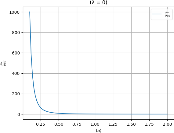
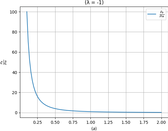
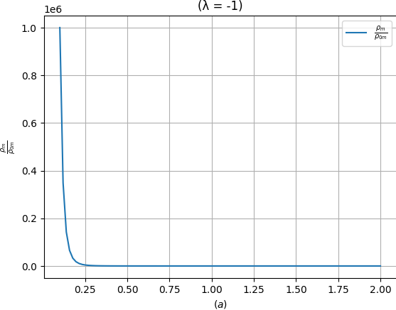

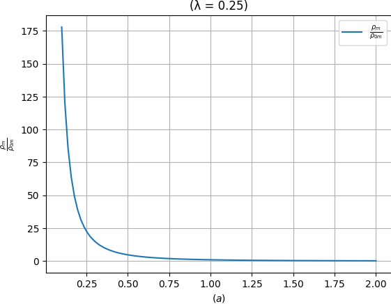
From the plot in Fig. 1, we can observe the behavior of the energy density ratios for matter and dark energy with respect to the scale factor (), assuming . Based on the observed behavior of the energy density ratios for dark matter and dark energy in the plot, we can conclude that dark energy and dark matter evolve independently according to their respective energy conservation equations. The fact that each component follows its expected dilution behavior without any significant deviations or interactions suggests that there is no direct energy exchange or strong interaction between dark energy and dark matter in this specific cosmological model. When dark energy dominates and its energy density decreases more slowly than matter, the universe’s expansion accelerates.For positive and negative values of , this behavior suggests that dark energy becomes relatively more significant compared to dark matter as the universe expands.
3.2 Dynamics of with
The equations that describe the dynamics of cosmology can be rephrased using a different variable known as the density parameter. This parameter is defined as the ratio of the energy density to the critical density and is mathematically expressed as:
| (21) |
In this equation, represents the Hubble parameter, which is the rate of expansion of the universe, and denotes the critical density. The value of provides valuable insights into the local characteristics of the universe. Particularly, when , the universe is regarded as having a flat spatial geometry. In cases where is less than 1, the universe exhibits a negatively curved geometry, whereas for greater than 1, a positively curved geometry characterizes the universe’s spatial structure.
Additionally, we can manipulate expressions using the chain rule, which is a fundamental concept in calculus. For any function with respect to cosmic time, its derivative with respect to can be written as:
| (22) |
This result remains consistent with the original equations and helps provide a deeper understanding of the relationships between various cosmological quantities. Thus, for , we are able to formulate the derivative of a function in relation to the in the subsequent manner:
| (23) |
Continuing, let us establish the notation and . This allows us to articulate the derivatives of and with respect to the natural logarithm of the scale factor as:
| (24) |
and
| (25) |
The expressions and represent the time derivatives of the energy densities of matter and the tachyon scalar field, respectively, while denotes the derivative of the Hubble parameter with respect to time. With these equations, we can explore the evolution of the density parameters for matter and the tachyon field as the scale factor changes. By analyzing the variations in these parameters, we gain insights into how matter and the tachyon field contribute to the dynamics of the universe with respect to time.
Using the (Eq.(12,15)), we get
| (26) | ||||
Using Friedmann Equation
| (27) |
| (28) |
Utilizing equations (26) and (28) and assuming a spatially flat universe where , we can simplify the differential equations (24) and (25) as follows:
| (29) |
| (30) |
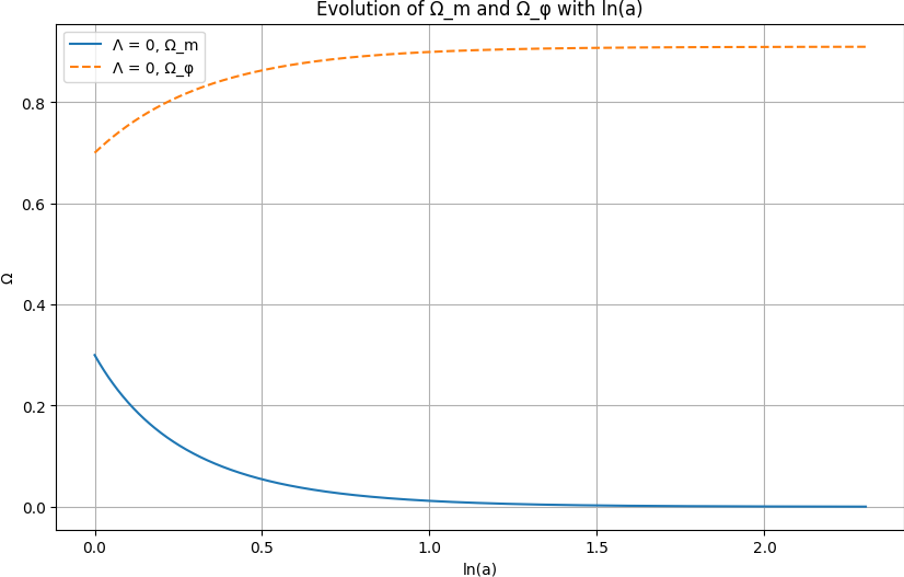
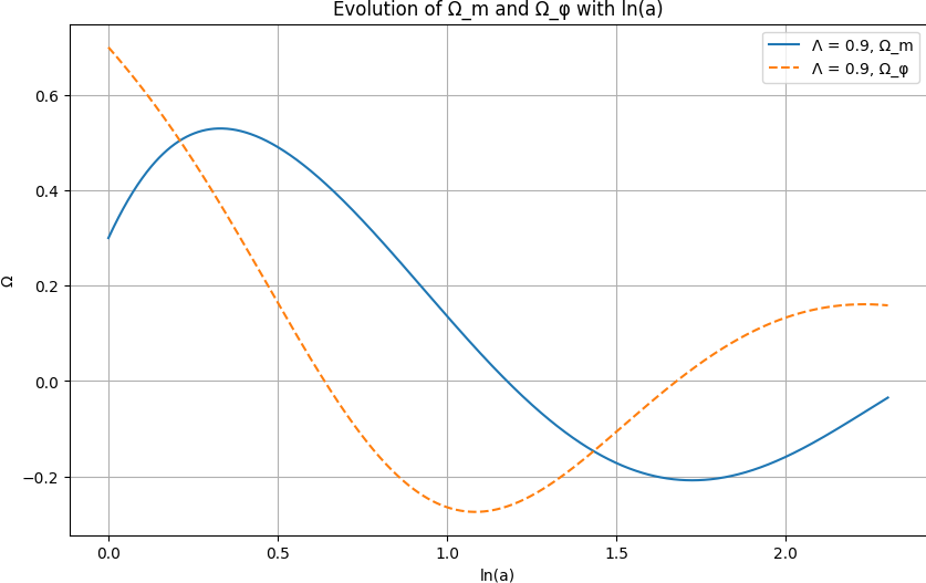
These equations represent the evolution of the density parameters (matter) and (scalar field or dark energy) with respect to the natural logarithm of the scale factor , given a constant . We can solve the provided equations by utilizing initial conditions: and , considering various values of . The evolution of and with respect to the natural logarithm of the scale factor is illustrated in Fig. (2).
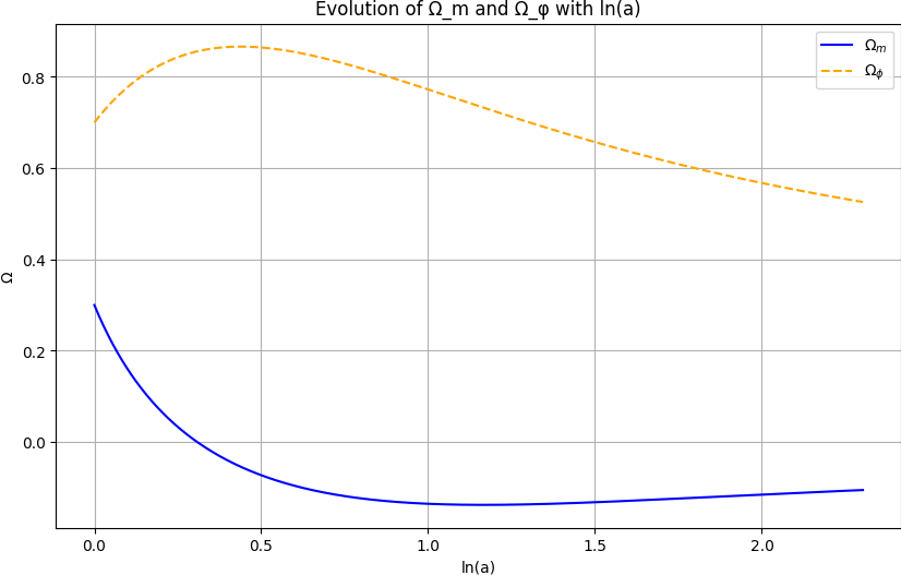
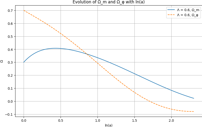
For , as increases (corresponding to the expansion of the universe), both and decrease. However, decreases at a slower rate than for this value of . This means that dark energy remains more significant compared to matter as the universe expands.
For , both and decrease as increases. However, in this case, decreases at a slightly faster rate compared to . This implies that dark energy remains more significant compared to matter, but the difference in their rates of decrease is small.
Both cases with and show that dark energy remains the dominant component in the universe, and matter becomes less significant as the universe expands. The difference lies in the rate at which dark energy remains dominant, with showing a slower decrease in dark energy compared to .
Zero Lambda ()**: When is zero, the equations simplify, and the density parameters evolve differently compared to the cases with non-zero lambda. Initially, decreases with the expansion of the universe, while remains constant. This is because dark energy does not interact with matter in this simplified case (). In the future, both and decrease, and they approach equality. This epoch is known as the ”epoch of matter-dark energy equality.”
For negative , the terms involving in the equations will lead to the opposite behavior compared to positive . Specifically, the terms involving will contribute to decreasing and increasing , leading to a reduction in the difference between and as becomes more negative. In other words, as becomes more negative, the influence of dark energy () becomes stronger compared to matter (), and the densities of both and tend to converge. This is why the difference between and decreases as becomes more negative.
4 Scale Factor Evolution
The variation of the scale factor with time is a fundamental aspect in understanding the dynamics of the universe’s expansion. It serves as a crucial link between cosmological quantities and plays a significant role in connecting functions of the scale factor and cosmic time . The Friedmann equation, a cornerstone in cosmology, establishes a vital relation between the scale factor and the energy density . The Friedmann equation, which is derived from the Einstein field equations, describes the overall expansion rate of the universe as a function of the energy content within it.
As the universe expands, the scale factor increases, signifying the stretching of space itself. This expansion directly affects the energy density, causing it to dilute over time. In turn, the evolution of influences the behavior of and, consequently, the rate at which the universe expands. Therefore, Friedmann Equation in Terms of Scale Factor can be written as :
| (31) |
| (32) |
Simplifying further,
| (33) |
| (34) |
| (35) |
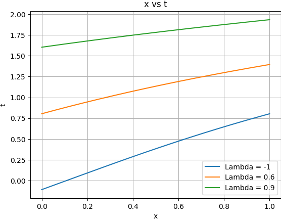
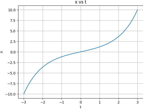
The plot highlights how the value of affects the expansion dynamics of the universe. For different values of , the scale factor evolves differently over time, leading to distinct shapes in the vs curves. The vs curves are continuous and smooth, reflecting the smooth and continuous nature of the expansion of the universe over time. As increases (moving from left to right on the x-axis), also increases, reflecting the expansion of the universe with time. For : The curve is smooth and continuously increasing, representing a universe with a cosmological constant ( corresponds to a de Sitter universe). For : The curve starts with a steeper slope, indicating a faster expansion at early times, and then the slope becomes less steep as increases. This behavior is typical of a universe with a combination of matter and dark energy. For : The curve starts with a gentle slope, representing slow expansion at early times, and then it becomes steeper as increases, indicating accelerated expansion at later times. This behavior is characteristic of a universe with a dominant dark energy component. For : Expanding Universe: The plot illustrates that as time () progresses, the scale factor () of the universe increases. This is consistent with the expanding nature of our universe, where galaxies, clusters, and structures are moving apart from each other over time. Acceleration of Expansion: The curve of the plot appears to have a positive slope, indicating that increases with at an accelerating rate. This behavior suggests that the universe’s expansion is accelerating, a phenomenon associated with the presence of dark energy. Early Universe Dynamics: The plot shows that as approaches zero (near the origin), the scale factor is also close to zero. This corresponds to the early stages of the universe when it was much smaller and denser during the Big Bang. Asymptotic Behavior: As approaches infinity (far right end of the plot), the scale factor increases, but it approaches a constant value. This implies that at very large timescales, the expansion of the universe approaches a steady state, known as the de Sitter space.
5 Cosmic Time Since Inception
The Age of the Universe (AOU) is a crucial parameter in cosmology, representing the time difference between the present day (when the scale factor is 1) and the moment of the Big Bang (when the scale factor was 0). Calculating the AOU involves finding the definite integral of the equation that describes the evolution of the scale factor over time. To elaborate further, the scale factor () is a fundamental quantity in cosmology that characterizes the expansion of the universe. It represents the relative size of the universe at different cosmic times. The value of at any given time tells us how much the universe has expanded compared to a reference time (usually the present).
The equation that governs the evolution of the scale factor is typically derived from the Friedmann equations, which describe the dynamics of an expanding universe in the context of general relativity. The specific form of the equation depends on the cosmological model and the energy components present in the universe (such as matter, dark energy, and radiation). To calculate the AOU, we need to integrate the time derivative of the scale factor () with respect to time () from the moment of the Big Bang (when ) to the present day (when ):
| (36) |
Using equation (34), we can write:
| (37) |
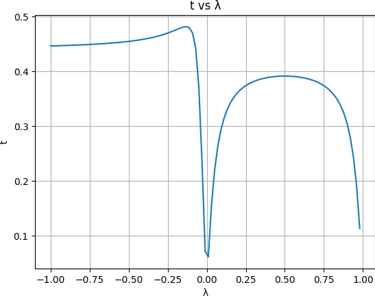
Based on the given plot, there are no apparent breaks or discontinuities in the age of the universe () as a function of the coupling parameter () in the range . The plot appears to be a continuous curve without any sudden jumps or discontinuous changes.
As there are no breaks or discontinuities in the age of the universe, there is no lower limit on the coupling parameter . The model remains valid for values as low as -1.
From Table 1, we can see that the upper limit on is . Beyond this value, the age of the universe starts to decrease and exhibits non-monotonic pattern with fluctuations in its values, which may lead to unphysical or unrealistic cosmological scenarios.
Mathematically,
The quantity can be calculated using the expression:
| (38) |
Now, let’s examine the values of and for close to and approaching 1:
| (39) |
| (40) |
As approaches 1, the value of will approach zero, and the value of will approach infinity. When approaches zero, the argument of the first term inside the parenthesis will approach zero, causing the first term to tend to zero. On the other hand, the second term will diverge to infinity as approaches infinity.
Therefore, to ensure that remains finite, we must have to prevent the divergence of as approaches 1. On the other hand, there is no lower limit on the coupling parameter in the graph. As approaches -1, the values of and will also approach negative infinity, but remains finite and continuous in this limit. There are no breaks or discontinuities in the age of the universe as a function of for approaching -1. Therefore, there is no lower limit on the coupling constant .
The upper limit is necessary to prevent the divergence of as approaches 1, while there is no lower limit on as remains continuous and finite for all values.
| AOU | AOU | ||
|---|---|---|---|
| -1 | 1.390 | 0 | 0.9206 |
| -0.9 | 1.393 | 0.1 | 0.966 |
| -0.8 | 1.396 | 0.2 | 1.130 |
| -0.7 | 1.400 | 0.3 | 1.190 |
| -0.6 | 1.406 | 0.4 | 1.216 |
| -0.5 | 1.415 | 0.5 | 1.221 |
| -0.4 | 1.427 | 0.6 | 1.216 |
| -0.3 | 1.447 | 0.7 | 1.190 |
| -0.2 | 1.478 | 0.8 | 1.130 |
| -0.1 | 1.488 | 0.9 | 0.966 |
6 Comparison of Coupling Strength
In our model, the interaction term can manifest in three distinct forms: , , and . Previous studies [22, 53] extensively investigated the first two forms, and they revealed that the coupling strength and can vary between any real value without a lower bound, but it must have an upper limit of 1. Similarly, the coupling strength in the third form of interaction, which is the focus of our analysis in this article, also has no lower bound but is bounded above and must be less than .
Interestingly, it is noteworthy that the possible range of values for , , and is , indicating that these coupling constants essentially represent the same physical parameter in our model, albeit with different notations. Consequently, they are interchangeable representations of the underlying physical quantity, reflecting the consistency and interrelated nature of these coupling constants in our theoretical framework.
7 Conclusion
In this comprehensive study, we delve into the dynamics of a universe featuring an interacting tachyonic scalar field (TSF) as a potential source of dark energy. Our model considers energy exchange between the scalar field and matter, with the interaction being linearly dependent on their combined energy densities. The evolution of energy densities concerning the scale factor is carefully analyzed, and we derive the density parameter () as a function of the natural logarithm of the scale factor. Furthermore, we express universe age in terms of the coupling constant .
A significant finding of this study is the consistency of constraints on lambda across all three cases considered. Whether the interaction depends on matter’s energy density, dark energy’s energy density, or a combination of both, the upper bound on lambda remains unchanged. This universality highlights the robustness of the constraint and suggests a universal upper limit for lambda, independent of the specific form of the interaction.
The agreement with prior research [22, 53] enhances the credibility of our approach, indicating that the interacting tachyonic scalar field model holds valuable insights into the dynamics of dark energy and its role in the universe’s accelerated expansion. Further investigations and refinements, coupled with observational data, have the potential to provide deeper understanding of the nature of the coupling constant and its implications for the evolution of the cosmos.
References
- [1] A. G. Riess, A. V. Filippenko, P. Challis, A. Clocchiatti, A. Diercks, P. M. Garnavich, R. L. Gilliland, C. J. Hogan, S. Jha, R. P. Kirshner, and et al., ”Observational evidence from supernovae for an accelerating universe and a cosmological constant,” The Astronomical Journal, vol. 116, p. 1009–1038, Sep 1998.
- [2] S. Perlmutter, G. Aldering, G. Goldhaber, R. A. Knop, P. Nugent, P. G. Castro, S. Deustua, S. Fabbro, A. Goobar, D. E. Groom, and et al., “Measurements of and from 42 high-redshift supernovae,” The Astrophysical Journal, vol. 517, p. 565–586, Jun 1999.
- [3] E. J. Copeland, M. Sami, and S. Tsujikawa, “Dynamics of dark energy,” International Journal of Modern Physics D, vol. 15, no. 11, pp. 1753–1935, 2006.
- [4] T. Padmanabhan and T. R. Choudhury, “Can the clustered dark matter and the smooth dark energy arise from the same scalar field?,” Physical Review D, vol. 66, no. 8, p. 081301, 2002.
- [5] M. M. Verma and S. D. Pathak, “Cosmic expansion driven by real scalar field for different forms of potential,” Astrophysics and Space Science, vol. 350, pp. 381–384, 2014.
- [6] M. M. Verma and S. D. Pathak, “The bicep2 data and a single higgs-like interacting scalar field,” International Journal of Modern Physics D, vol. 23, no. 09, p. 1450075, 2014.
- [7] M. Cruz, S. Lepe, and G. E. Soto, “Phantom cosmologies from qcd ghost dark energy,” Physical Review D, vol. 106, no. 10, p. 103508, 2022.
- [8] S. Narawade and B. Mishra, “Phantom cosmological model with observational constraints in f (q) gravity,” arXiv preprint arXiv:2211.09701, 2022.
- [9] S. Tripathy and B. Mishra, “Phantom cosmology in an extended theory of gravity,” Chinese Journal of Physics, vol. 63, pp. 448–458, 2020.
- [10] V. B. Johri, “Phantom cosmologies,” Physical Review D, vol. 70, no. 4, p. 041303, 2004.
- [11] M. P. D browski, C. Kiefer, and B. Sandhoefer, “Quantum phantom cosmology,” Physical Review D, vol. 74, no. 4, p. 044022, 2006.
- [12] M. P. Dabrowski, T. Stachowiak, and M. Szyd lowski, “Phantom cosmologies,” Physical Review D, vol. 68, no. 10, p. 103519, 2003.
- [13] A. Adil, A. Albrecht, and L. Knox, “Quintessential cosmological tensions,” Physical Review D, vol. 107, no. 6, p. 063521, 2023.
- [14] W. Yang, M. Shahalam, B. Pal, S. Pan, and A. Wang, “Constraints on quintessence scalar field models using cosmological observations,” Physical Review D, vol. 100, no. 2, p. 023522, 2019.
- [15] C. Wetterich, “The quantum gravity connection between inflation and quintessence,” Galaxies, vol. 10, no. 2, p. 50, 2022.
- [16] E. Piedipalumbo, M. De Laurentis, and S. Capozziello, “Noether symmetries in interacting quintessence cosmology,” Physics of the Dark Universe, vol. 27, p. 100444, 2020.
- [17] F. Felegary, I. Akhlaghi, and H. Haghi, “Evolution of matter perturbations and observational constraints on tachyon scalar field model,” Physics of the Dark Universe, vol. 30, p. 100739,2020.
- [18] A. Singh, A. Sangwan, and H. Jassal, “Low redshift observational constraints on tachyon models of dark energy,” Journal of Cosmology and Astroparticle Physics, vol. 2019, no. 04, p. 047, 2019.
- [19] M. Koussour and M. Bennai, “Interacting tsallis holographic dark energy and tachyon scalar field dark energy model in bianchi type-ii universe,” International Journal of Modern Physics A, vol. 37, no. 05, p. 2250027, 2022.
- [20] J. Sadeghi, M. Khurshudyan, M. Hakobyan, and H. Farahani, “Phenomenological fluids from interacting tachyonic scalar fields,” International Journal of Theoretical Physics, vol. 53, pp. 2246– 2260, 2014.
- [21] V. Gorini, A. Kamenshchik, U. Moschella, and V. Pasquier, “Tachyons, scalar fields, and cosmology,” Physical Review D, vol. 69, no. 12, p. 123512, 2004.
- [22] A. Kundu, S. Pathak, and V. Ojha, “Interacting tachyonic scalar field,” Communications in Theoretical Physics, vol. 73, no. 2, p. 025402, 2021.
- [23] D. R. Kumar, S. D. Pathak, and V. K. Ojha, “Gauging universe expansion via scalar fields,” Chin. Phys. C, vol. 47, no. 5, p. 055102, 2023.
- [24] A. Sen, “Rolling tachyon,” Journal of High Energy Physics, vol. 2002, p. 048–048, Apr 2002.
- [25] A. Sen, “Tachyon matter,” Journal of High Energy Physics, vol. 2002, p. 065–065, Jul 2002.
- [26] A. Sen, “Field theory of tachyon matter,” Modern Physics Letters A, vol. 17, p. 1797–1804, Sep2002.
- [27] L. P. Chimento, “Linear and nonlinear interactions in the dark sector,” Physical Review D, vol. 81, p. 043525, Feb 2010.
- [28] L. P. Chimento, M. Forte, and G. M. Kremer, “Cosmological model with interactions in the dark sector,” General Relativity and Gravitation, vol. 41, p. 1125–1137, Sep 2008.
- [29] O. Bertolami, P. Carrilho, and J. P´aramos, “Two-scalar-field model for the interaction of dark energy and dark matter,” Physical Review D, vol. 86, p. 103522, Nov 2012.
- [30] B. Wang, J. Zang, C.-Y. Lin, E. Abdalla, and S. Micheletti, “Interacting dark energy and dark matter: Observational constraints from cosmological parameters,” Nuclear Physics B, vol. 778, p. 69–84, Aug 2007.
- [31] J. Lu, Y. Wu, Y. Jin, and Y. Wang, “Investigate the interaction between dark matter and dark energy,” Results Phys., vol. 2, pp. 14–21, 2012, 1203.4905.
- [32] H. Farajollahi, A. Ravanpak, and G. Fadakar, “Interacting agegraphic dark energy model in tachyon cosmology coupled to matter,” Physics Letters B, vol. 711, p. 225–231, May 2012.
- [33] W. Zimdahl, “Models of interacting dark energy,” AIP Conf. Proc., vol. 1471, pp. 51–56, 2012, 1204.5892.
- [34] W. Yang, S. Pan, E. D. Valentino, R. C. Nunes, S. Vagnozzi, and D. F. Mota, “Tale of stable interacting dark energy, observational signatures, and the h0 tension,” Journal of Cosmology and Astroparticle Physics, vol. 2018, p. 019–019, Sep 2018.
- [35] S. Cao, N. Liang, and Z.-H. Zhu, “Testing the phenomenological interacting dark energy with observational data,” Monthly Notices of the Royal Astronomical Society, vol. 416, p. 1099–1104,Jul 2011.
- [36] E. Di Valentino, A. Melchiorri, O. Mena, and S. Vagnozzi, “Nonminimal dark sector physics and cosmological tensions,” Physical Review D, vol. 101, p. 063502, Mar 2020.
- [37] M. M. Verma and S. D. Pathak, “A tachyonic scalar field with mutually interacting components,” International Journal of Theoretical Physics, vol. 51, p. 2370–2379, Mar 2012.
- [38] M. M. Verma and S. D. Pathak, “Shifted cosmological parameter and shifted dust matter in a two-phase tachyonic field universe,” Astrophysics and Space Science, vol. 344, p. 505–512, Jan 2013.
- [39] J. V¨aliviita, R. Maartens, and E. Majerotto, “Observational constraints on an interacting dark energy model,” Monthly Notices of the Royal Astronomical Society, vol. 402, p. 2355–2368, Mar 2010.
- [40] S. Pan, A. Mukherjee, and N. Banerjee, “Astronomical bounds on a cosmological model allowing a general interaction in the dark sector,” Monthly Notices of the Royal Astronomical Society, vol. 477, p. 1189–1205, Mar 2018.
- [41] L. Amendola, J. Rubio, and C. Wetterich, “Primordial black holes from fifth forces,” Physical Review D, vol. 97, p. 081302, Apr 2018.
- [42] D. B´egu´e, C. Stahl, and S.-S. Xue, “A model of interacting dark fluids tested with supernovae and baryon acoustic oscillations data,” Nuclear Physics B, vol. 940, p. 312–320, Mar 2019.
- [43] S. Pan, W. Yang, C. Singha, and E. N. Saridakis, “Observational constraints on sign-changeable interaction models and alleviation of the h0 tension,” Physical Review D, vol. 100, p. 083539, Oct 2019.
- [44] G. Papagiannopoulos, P. Tsiapi, S. Basilakos, and A. Paliathanasis, “Dynamics and cosmological evolution in -varying cosmology,” The European Physical Journal C, vol. 80, p. 55, Jan 2020.
- [45] S. Savastano, L. Amendola, J. Rubio, and C. Wetterich, “Primordial dark matter halos from fifth forces,” Physical Review D, vol. 100, p. 083518, Oct 2019.
- [46] R. von Marttens, L. Casarini, D. Mota, and W. Zimdahl, “Cosmological constraints on parametrized interacting dark energy,” Physics of the Dark Universe, vol. 23, p. 100248, Jan 2019.
- [47] W. Yang, N. Banerjee, A. Paliathanasis, and S. Pan, “Reconstructing the dark matter and dark energy interaction scenarios from observations,” Phys. Dark Univ., vol. 26, p. 100383, 2019, 1812.06854.
- [48] M. Asghari, J. B. Jim´enez, S. Khosravi, and D. F. Mota, “On structure formation from a small-scales-interacting dark sector,” Journal of Cosmology and Astroparticle Physics, vol. 2019, p. 042–042, Apr 2019.
- [49] M. Shahalam, S. Pathak, S. Li, R. Myrzakulov, and A. Wang, “Dynamics of coupled phantom and tachyon fields,” The European Physical Journal C, vol. 77, pp. 1–12, 2017.
- [50] M. Shahalam, S. Pathak, M. Verma, M. Y. Khlopov, and R. Myrzakulov, “Dynamics of interacting quintessence,” The European Physical Journal C, vol. 75, pp. 1–9, 2015.
- [51] D. Pav´on and B. Wang, “Le chˆatelier–braun principle in cosmological physics,” General Relativity and Gravitation, vol. 41, p. 1–5, Jun 2008.
- [52] R. De Arcia, I. Quiros, U. Nucamendi, T. Gonzalez, F. A. Horta-Rangel, and P. Eenens, “Global asymptotic dynamics of the cubic galileon interacting with dark matter,” Phys. Dark Univ., vol. 40, p. 101183, 2023, 2206.14333
- [53] Ojha, V. K., Rao, A. A., and Pathak, S. D. (2023). Interacting tachyonic scalar field II. arXiv preprint arXiv:2305.00277.
