From the random geometry of conformally invariant systems to the Kähler geometry of universal Teichmüller space
submitted for Notices of the American Mathematical Society

Scaling limits of critical lattice models provide several important examples of conformally invariant random self-avoiding curves. Examples include loop-erased random walk, spin cluster interfaces in the critical Ising model, and the level line of a discrete Gaussian free field. We would like to describe what lattice size scaling limits of such curves may look like. Physicists predict that conformal invariance emerge for a wide-range of well-chosen statistical mechanics models [1]. For instance, the simple random walk in $\delta\mathbb{Z}^{2}$ converges in the scaling limit (when $\delta\to 0$) to the planar Brownian motion, whose trajectory is indeed conformally invariant up to reparametrization. However, since we deal with self-avoiding paths, any scaling limit should still be non-self-crossing, so cannot be a Markov process. (The future path of a Markov process only depends on the current location. For instance, the trajectory of a Brownian motion in $\mathbb{R}^{2}$ almost surely hits itself infinitely many times on arbitrarily small time interval.)

By considering properties expected from the discrete models as predicted by physics, O. Schramm formulated a mathematical description of random simple curves with conformal symmetries [13]. It turns out to be convenient to first assume that the random simple curve connects two distinct boundary points (prime ends) $a,b$ in a simply connected domain $D\subsetneq\mathbb{C}$. We call such a simple curve a chord in $(D;a,b)$ and oriented from $a$ to $b$. This setup will allow us to progressively slit open the curve starting from $a$, and so that the remaining part of the curve will be a chord connecting the endpoint of the slit and $b$ in the slit domain.

One advantage of working in two dimensions is that there is a rich family of conformal maps, given by biholomorphic functions (so we may use single-variable complex analysis). In particular, the Riemann mapping theorem states that there exists a conformal map $\varphi$ sending the simply connected domain $D$ to the upper half-plane $\mathbb{H}=\{z\in\mathbb{C}\colon\operatorname{Im}(z)>0\}$, which maps $a$ to $0\in\partial\mathbb{H}=\mathbb{R}\cup\{\infty\}$ and $b$ to $\infty\in\partial\mathbb{H}$. Another choice of such conformal map has to be of the form $\lambda\varphi$ for some $\lambda>0$.

Schramm realized that the random simple chord has to satisfy two properties:

• •

  Conformal invariance: The random chord $\gamma$ in $\mathbb{H}$ connecting $0$ to $\infty$ should have the same law as its image under the map $z\mapsto\lambda z$ for every $\lambda>0$. This then allows us to define the random chord in $(D;a,b)$ as the preimage under any $\varphi:D\to\mathbb{H}$.

• •

  Domain Markov property: Chords of $(\mathbb{H};0,\infty)$ have a parametrization by capacity (explained below). If we slit the random chord $\gamma$ in $(\mathbb{H};0,\infty)$ from $\gamma(0)=0$ up to $\gamma(s)$ and map conformally $(\mathbb{H}\smallsetminus\gamma[0,s];\gamma(s),\infty)$ to $(\mathbb{H};0,\infty)$, then the image of $\gamma[s,\infty)$ should have the same law as $\gamma$ and be independent of $\gamma[0,s]$, for every $s>0$.

Indeed, many scaling limits of the interfaces in critical lattice models are proved to satisfy these axioms, e.g., [9, 14]. However, we do not need to invoke discrete models if we use these two properties as the axiomatic definition of the random chord of interest in the continuum. Schramm noticed that the Loewner transform [10] provides a perfect tool to describe it. The Loewner transform encodes any given chord in $(\mathbb{H};0,\infty)$ into a continuous real-valued function. More precisely, we say that $\gamma$ is parametrized by capacity if the unique conformal map $g_{t}:\mathbb{H}\smallsetminus\gamma[0,t]\to\mathbb{H}$, normalized such that the expansion at infinity is given by $g_{t}(z)=z+o(1)$, has in fact the next term in the expansion being $2t/z$, namely,

$$g_{t}(z)=z+\frac{2t}{z}+o\Big(\frac{1}{z}\Big).$$

The image of the tip $\gamma(t)$ of $\gamma[0,t]$ under $g_{t}$ is denoted as $W_{t}\in\mathbb{R}$. Let $T\in(0,\infty]$ be the total capacity of $\gamma$. As $t$ varies in $[0,T)$, $t\mapsto W_{t}$ is continuous and starting from $W_{0}=0$. We call $W$ the Loewner driving function of $\gamma$. Moreover, for each $z\in\mathbb{H}$, $t\mapsto g_{t}(z)$ satisfies a simple differential equation $\partial_{t}g_{t}(z)=2/(g_{t}(z)-W_{t})$ with the initial condition $g_{0}(z)=z$. This allows us to recover $\gamma$ from $W$.

It is a simple exercise to check that the two properties of the random simple chord above translate into the following properties of the random continuous driving function $W$:

• •

  $W$ has the same law as the function $t\mapsto\lambda W_{\lambda^{-2}t}$, for every $\lambda>0$;

• •

  for every $s>0$, $t\mapsto W_{t+s}-W_{s}$ has the same law as $W$ and is independent of $W|_{[0,s]}$.

The first condition implies that $T=\infty$ almost surely. It turns out the only possible random continuous function satisfying these properties is of the form of $\sqrt{\kappa}B$, where $B$ is the standard Brownian motion and $\kappa\geq 0$. In fact, the second property guarantees $W$ to be a continuous Lévy process. The classification of continuous Lévy processes tells us that it is of the form $t\mapsto\sqrt{\kappa}B_{t}+at$, for some $a\in\mathbb{R}$. One may view the classification as the manifestation of two most fundamental theorems in probability theory: the law of large numbers (which explains the occurrence of the deterministic drift $t\mapsto at$), central limit theorem (which explains the occurrence of the Gaussian process $\sqrt{k}B$). Since Brownian motion satisfies the first property which transforms the drift $at$ into $\lambda^{-1}at$, it implies that $\lambda^{-1}a=a$ which shows $a=0$.

Schramm–Loewner evolution $\operatorname{SLE}_{\kappa}$ in $(\mathbb{H};0,\infty)$ is the random curve whose driving function is $\sqrt{\kappa}B$, for some $\kappa\geq 0$. More precisely, when $\kappa\leq 4$, SLE_κ is indeed the random simple chord with driving function $\sqrt{\kappa}B$ in the sense described above; for $\kappa>4$, the Loewner driving function does not define a growing slit $\gamma[0,t]$ but a growing compact set $K_{t}\subset\overline{\mathbb{H}}$. In this case, SLE_κ is referred to as the curve which carves out progressively the boundary of $K_{t}$ (when $\kappa\geq 8$, SLE_κ is a random space-filling curve) [11]. We will only consider the case where $\kappa\leq 4$ and do not enter into further details to discuss the $\kappa>4$ case. The SLE_κ in another domain $(D;a,b)$ is defined as the preimage of $\operatorname{SLE}_{\kappa}$ in $(\mathbb{H};0,\infty)$ under any conformal map $\varphi:D\to\mathbb{H}$ sending respectively $a,b$ to $0,\infty$.

From the discussion above, SLE curves are the only possible non-self-crossing curves appearing in conformally invariant systems which satisfy conformal invariance and domain Markov property. The study of SLE curves and their variants, as well as the connections to random surfaces, discrete models, and conformal field theory has grown into a thriving field of two-dimensional random conformal geometry. We refer the reader to the textbooks, e.g., [19], which provide detailed introductions to SLEs and applications.

We will slowly move away from the probability world by only looking at a deterministic functional that arises from large deviation principles of SLE. Interested readers may consult [18] for a more complete survey on this topic.

Large deviation principles capture the exponential decay of the probability of rare events. A classical example is the large deviation principle of the Brownian motion: Schilder’s theorem states that the probability of $\sqrt{\kappa}B$ staying close to a given deterministic real-valued function $W$ decays exponentially fast as $\kappa\to 0{\scriptstyle+}$ (when $W$ is not the zero function):

$$\lim_{\varepsilon\to 0}\lim_{\kappa\to 0}-\kappa\log\mathbb{P}(\sqrt{\kappa}B\text{ stays $\varepsilon$-close to }W)=I(W),$$

where $I(\cdot)$ is called the large deviation rate function of $(\sqrt{\kappa}B)_{\kappa\to 0{\scriptstyle+}}$ and is given by the Dirichlet energy

$$I(W):=\frac{1}{2}\int_{0}^{\infty}\dot{W}_{t}^{2}\,\mathrm{d}t,$$

where $\dot{W}_{t}:=\mathrm{d}W_{t}/\mathrm{d}t$ if $W$ is absolutely continuous, and $I(W)=\infty$ otherwise. Here, by $\varepsilon$-close we mean being in a ball of radius $\varepsilon$ with respect to a metric on $C^{0}([0,\infty))$ inducing uniform convergence on compact subsets.

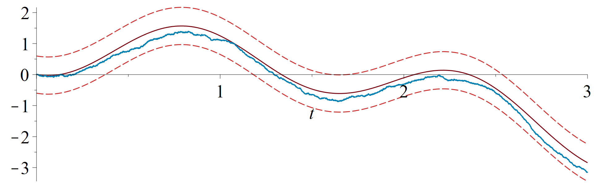
Given Schilder’s theorem, it is not surprising that using an appropriate metric, e.g., the Hausdorff metric, a similar large deviation principle holds for $\operatorname{SLE}_{0+}$: given a chord $\gamma$ in the domain $(D;a,b)$,

$$\lim_{\varepsilon\to 0}\lim_{\kappa\to 0}-\kappa\log\mathbb{P}(\operatorname{SLE}_{\kappa}\text{ in }(D;a,b)\text{ stays $\varepsilon$-close to }\gamma)=I_{D;a,b}^{C}(\gamma).$$

(1)

Here $I^{C}_{D;a,b}(\gamma):=I(W)$ is called the chordal Loewner energy of $\gamma$, where $W$ is the driving function of $\varphi(\gamma)$ and $\varphi$ is any conformal map sending $(D;a,b)$ onto $(\mathbb{H};0,\infty)$.

In a collaboration with Rohde, we generalized the Loewner energy to Jordan curves (simple loops) and realized that it shows more symmetries in this setup [12]. We will focus on the energy for Jordan curves from now and denote it as $I^{L}$. The energy for Jordan curve generalizes the chordal energy because of the following property:

$$I^{L}(\gamma\cup\mathbb{R}_{+})=I^{C}_{\mathbb{C}\smallsetminus\mathbb{R}_{+};0,\infty}(\gamma)$$

(2)

for every simple chord $\gamma$ in $(\mathbb{C}\smallsetminus\mathbb{R}_{+};0,\infty)$. The Loewner energy for a Jordan curve is defined as follows.

In fact, rather surprisingly, the definition does not depend on the choice of the orientation of the curve nor on its root [12]. Therefore, we omit the root from the notation and simply call $I^{L}(\gamma)$ the Loewner energy of $\gamma$. The relation (2) can be seen by putting the root at $\infty$ and orient the curve from $\infty\to 0$ along $\mathbb{R}_{+}$. The independence of the Loewner energy from the parametrization is not obvious, since the chordal energies $I^{C}$ are defined using the Loewner driving function which depends strongly on the past of the curve. This independence suggests that there must be an intrinsic expression of the Loewner energy which does not use any particular parametrization of the Jordan curve. The answer is given by the identity with the universal Liouville action that will be the subject of the next section.

We remark that since the Loewner energy is defined via uniformizing maps (to define the driving function), it is invariant under conformal automorphisms of $\hat{\mathbb{C}}$ (i.e., Möbius transformations $z\mapsto(az+b)/(cz+d)$). Moreover, the Loewner energy is zero if and only if $\gamma$ is a circle on $\hat{\mathbb{C}}$. Therefore, the Loewner energy may be viewed as a quantity measuring the roundness of the unparametrized Jordan curve.

The loop energy is, as one may guess, related to the loop version of SLE_κ. Indeed, the SLE_κ loop measure $\mu^{\kappa}$ was constructed in [20], and in this case, the link to the Loewner energy actually holds without letting $\kappa$ go to $0$. A recent work [5] shows that for a fixed $\kappa\leq 4$,

$\displaystyle\lim_{\varepsilon\rightarrow 0}\frac{\mu^{\kappa}\left(O_{\varepsilon}(\gamma)\right)}{\mu^{\kappa}\left(O_{\varepsilon}(S^{1})\right)}=\exp\left(\frac{c(\kappa)}{24}I^{L}(\gamma)\right),$

(4)

where $c(\kappa):=(6-\kappa)(3\kappa-8)/2\kappa$ is the central charge (terminology coming from the connection to conformal field theory) of $\operatorname{SLE}_{\kappa}$, $S^{1}$ is the unit circle, and $O_{\varepsilon}$ is a certain $\varepsilon$-neighborhood of $\gamma$ in the space of loops. In other words, $(c(\kappa)/24)I^{L}$ is the Onsager–Machlup action functional of the SLE_κ loop measure. On may also check that as $\kappa\to 0{\scriptstyle+}$, $c(\kappa)\sim-24/\kappa$ and we recover the asymptotics similar to (1).

We will focus on the Loewner energy for Jordan curves (and forget about its relation to SLE for a moment). The following theorem gives an equivalent expression the Loewner energy which does not use the Loewner transform. Since the Loewner energy is invariant under Möbius transformations, without loss of generality, we may assume that the Jordan curve $\gamma$ does not pass through $\infty$.

The quantity $\mathbf{S}$ was introduced in [15] under the name universal Liouville action. Its value does not depend on the choice of $f$ and $g$ as long as $g(\infty)=\infty$. A Jordan curve for which $\int_{\mathbb{D}}|f^{\prime\prime}/f^{\prime}|^{2}\,\mathrm{d}^{2}z$ is finite is called a Weil–Petersson quasicircle. It turns out that $\int_{\mathbb{D}}|f^{\prime\prime}/f^{\prime}|^{2}\,\mathrm{d}^{2}z$ is finite if and only if $\int_{\mathbb{D}^{*}}|g^{\prime\prime}/g^{\prime}|^{2}\,\mathrm{d}^{2}z$ is finite. Hence, we have:

We note that Weil–Petersson quasicircles are rectifiable. Therefore, finite Loewner energy curves are more regular than SLE_κ curves, which have Hausdorff dimension $(1+\kappa/8)\wedge 2$. This is not surprising as functions with finite Dirichlet energy are also more regular than a Brownian path which has infinite Dirichlet energy almost surely.

As mentioned above, the universal Liouville action does not depend on any special point on the curve $\gamma$ and has the advantage of involving only two conformal maps. Whereas to define the Loewner energy through the driving function, one has to study the whole family of uniformizing conformal mappings of the slit domains. However, the way of considering the Jordan curve as a progressively growing slit (which closes up on itself) allows us to relate the Loewner energy to SLE curves.

The universal Liouville action arises from a very different context — Teichmüller theory. Teichmüller spaces were introduced by Teichmüller to parametrize the family of complex structures on a surface using quasiconformal mappings. In particular, the Teichmüller space of a genus $g\geq 2$ closed surface is homeomorphic to $\mathbb{R}^{6g-6}$. The universal Teichmüller space is infinite-dimensional and contains all Teichmüller spaces of surfaces of negative Euler characteristics, hence the name universal, which can also be represented by the class of quasicircles.

More precisely, we first identify a Jordan curve $\gamma$ with a homeomorphism of the unit circle $S^{1}=\partial\mathbb{D}=\partial\mathbb{D}^{*}$ as follows. By Carathéodory’s theorem, any conformal map $f:\mathbb{D}\to\Omega$ (resp., $g:\mathbb{D}^{*}\to\Omega^{*}$) extends continuously to a homeomorphism between the closures $\overline{\mathbb{D}}\to\overline{\Omega}$ (resp., $\overline{\mathbb{D}^{*}}\to\overline{\Omega^{*}}$). In particular, $f$ and $g$ restricted to $S^{1}$ define two homeomorphisms $S^{1}\to\gamma$. The welding homeomorphism, defined as the circle homeomorphism $\varphi:=g^{-1}\circ f|_{S^{1}}$, compares these two homeomorphisms.

The converse operation — solving the conformal welding problem — consists of finding a Jordan curve $\gamma$ and corresponding conformal maps $f$ and $g$, whose welding homeomorphism $g^{-1}\circ f|_{S^{1}}$ is a given circle homeomorphism $\varphi$. We note that if $\gamma$ is a solution, then $A\circ\gamma$ is also a solution (by replacing $f$ by $A\circ f$ and $g$ by $A\circ g$), where $A$ is any Möbius transformation of $\hat{\mathbb{C}}$. A solution may not exist, and if one exists, it may not be unique (up to post-composition by Möbius transformations). The complete characterization of circle homeomorphisms for which there is a unique solution to conformal welding is a hard open question: Bishop showed that those corresponding Jordan curves form a set which is not Borel measurable.

However, it is classical that if the circle homeomorphism is quasisymmetric, then the solution to the conformal welding problem exists and is unique up to post-composition by Möbius transformations. We use

$$\mathord{\raise 0.49991pt\hbox{$\displaystyle\operatorname{QS}(S^{1}):=\left\{\varphi\in\operatorname{Hom}(S^{1})\colon\exists M>1,\,\forall\theta\in\mathbb{R},\,\forall t\in(0,\pi),\,\genfrac{}{}{0.4pt}{}{1}{M}\leq\left\lvert\genfrac{}{}{0.4pt}{}{\varphi(e^{\ii(\t+ t)}) -\varphi( e^{\ii\t})}{\varphi(e^{\ii\t} )- \varphi(e^{\ii(\t-t)})}\right\rvert\leq M\right\}$}}$$

to denote the group of quasisymmetric circle homeomorphisms. The corresponding Jordan curves are called quasicircles.

Let $\varphi\in\operatorname{QS}(S^{1})$ and consider its solution to the welding problem. We fix a normalization by assuming that the conformal map $f$ satisfies $f(0)=0,f^{\prime}(0)=1$ and $f^{\prime\prime}(0)=0$ and put no condition on $g$ (except that $g(\mathbb{D}^{*})=\hat{\mathbb{C}}\smallsetminus\overline{f(\mathbb{D})}$). In other words, we consider the welding homeomorphism to be in the homogeneous space $\mathrm{M\ddot{o}b}(S^{1})\backslash\operatorname{QS}(S^{1})$, where $\mathrm{M\ddot{o}b}(S^{1})$ is the group of Möbius transformations preserving $S^{1}$ (since $g$ can be replaced by $g\circ B$ for any $B\in\mathrm{M\ddot{o}b}(S^{1})$). The homogeneous space $T(1):=\mathrm{M\ddot{o}b}(S^{1})\backslash\operatorname{QS}(S^{1})$ is called the universal Teichmüller space.

Universal Teichmüller space has an infinite dimensional complex Banach manifold structure such that the group $\operatorname{QS}(S^{1})$ acts on the right on $T(1)$ holomorphically. One wonders whether it can be further equipped with a Kähler metric, namely, a symplectic form $\omega(\cdot,\cdot)$ and Riemannian metric $\left\langle\cdot,\cdot\right\rangle$ that are invariant under the right action and compatible with the complex structure (encoded in an operator $J$ on the tangent bundle such that $J^{2}=-\operatorname{Id}$ which plays the role of “multiplication by $\mathfrak{i}$”). Being compatible means $\omega(\cdot,J(\cdot))=\left\langle\cdot,\cdot\right\rangle$. This question was motivated by string theory, e.g., [3], who consider only the smooth part $\mathrm{M\ddot{o}b}(S^{1})\backslash\operatorname{Diff}^{\infty}(S^{1})$ of the universal Teichmüller space without having to worry about any convergence issue on this infinite dimensional manifold. It turns out there is a unique Kähler metric up to a scaling factor.

Let us explain briefly how to derive this Kähler metric (also ignoring the convergence question). Concretely, the tangent space at $[\operatorname{Id}]\in T(1)$ consists of real vector fields Vect$(S^{1})$ on $S^{1}$ with Fourier expansion:

$$v=\sum_{n\neq\pm 1,0}v_{n}e^{\mathfrak{i}n\theta}\frac{\partial}{\partial\theta}=\sum_{n\neq\pm 1,0}v_{n}e_{n}\quad\text{ satisfying }\overline{v}_{n}=v_{-n}\in\mathbb{C},$$

where $e_{n}:=e^{\mathfrak{i}n\theta}\partial/\partial\theta$. We have omitted the Fourier modes for $n\in\{\pm 1,0\}$ as they generate the Lie algebra of $\mathrm{M\ddot{o}b}(S^{1})$.

The almost complex structure $J:\text{Vect}(S^{1})\to\text{Vect}(S^{1})$ (such that $J^{2}=-\operatorname{Id}$) induced from the complex structure is given by the Hilbert transform:

$$Jv=\mathfrak{i}\sum_{n=2}^{\infty}v_{n}e_{n}-\mathfrak{i}\sum_{n=-\infty}^{-2}v_{n}e_{n}.$$

The $\mathbb{C}$-basis $\{e_{n}\}_{n\neq\pm 1,0}$ of the space of complexified vector fields has the Lie bracket

$$[e_{m},e_{n}]=\mathfrak{i}(n-m)e_{n+m}.$$

Takhtajan and Teo [15] extended the infinite-dimensional Kähler manifold structure and the Weil–Petersson metric to $T(1)$. In fact, the subspace of $u\in\text{Vect}(S^{1})$ such that $\left\langle u,u\right\rangle<\infty$ coincides with the $H^{3/2}$ Sobolev space of vector fields (which is strictly smaller than the tangent space of $T(1)$ which is given by the space of Zygmund vector fields).

So, $T_{0}(1)$ is the completion of $\mathrm{M\ddot{o}b}(S^{1})\backslash\operatorname{Diff}^{\infty}(S^{1})$. Moreover, a Jordan curve is associated with an element in $T_{0}(1)$ via conformal welding if and only if it is a Weil–Petersson quasicircle. There are many equivalent characterizations of the elements in $T_{0}(1)$, see, e.g., [2] for an extensive summary including several geometric characterizations. One special feature of Kähler metrics is that they always admit locally defined Kähler potential. Here, the Weil–Petersson metric has a globally defined potential given by the universal Liouville action:

This shows all information about the unique Kähler metric on $T_{0}(1)$ is recorded in the universal Liouville action, hence, the Loewner energy.

We now explain how we could come up with the identity between the Loewner energy and the universal Liouville action in Theorem 2 using ideas from random conformal geometry. The first step to guess the following identity for a Jordan curve passing through $\infty$.

This theorem can be viewed as a deterministic finite energy analog of the quantum zipper coupling between SLE and Gaussian free field (GFF) [7, 6] that we now explain. We do not make rigorous statements and only argue heuristically here.

Gaussian free field on a two-dimensional domain is a random real-valued Gaussian Schwartz distribution and the analog of Brownian motion by replacing the time interval by the domain. Similar to Schilder’s theorem, the large deviation rate function for $(\sqrt{k}\Phi)_{\kappa\to 0{\scriptstyle+}}$, where $\Phi$ is a free boundary GFF on a two-dimensional domain $D$, is the associated Dirichlet energy:

$$\mathcal{D}_{D}(\varphi):=\frac{1}{4\pi}\int_{D}|\nabla\varphi|^{2}\mathrm{d}^{2}z\in[0,\infty],\qquad\forall\varphi\in W^{1,2}_{loc}.$$

If $\mathcal{D}_{D}(\varphi)<\infty$, we say that $\varphi\in\mathcal{E}(D)$. A $\sqrt{\kappa}$-quantum surface is a two-dimensional domain $D$ equipped with a Liouville quantum gravity measure (denoted as $\sqrt{\kappa}$-LQG), defined using a regularization of $e^{\sqrt{\kappa}\Phi}\mathrm{d}^{2}z$, where $\sqrt{\kappa}\in(0,2)$.

We use the following dictionary illustrating the analogy between the concepts in random conformal geometry (left column) and their finite energy counterparts (right column). For a more complete dictionary and background, we refer the readers to [16, 18] and the references therein.

In the last line, two domains $D$ and $D^{\prime}$ equipped with a measure are considered equivalent if there exist a conformal map $D\to D^{\prime}$ such that the measure on $D^{\prime}$ equals the pushforward of the measure on $D$. In particular, if a Jordan curve $\gamma$ cuts $\mathbb{C}$ into two domains $H$ and $H^{*}$ as above and $f$ and $g$ are the conformal maps in Theorem 7, then $e^{2\varphi}\mathrm{d}^{2}z$ on $H$ and on $H^{*}$ are equivalent, respectively, to $e^{2u}\mathrm{d}^{2}z$ on $\mathbb{H}$ and $e^{2v}\mathrm{d}^{2}z$ on $\mathbb{H}^{*}$ where

$$u=\varphi\circ f+\log\left\lvert f^{\prime}\right\rvert,\quad v=\varphi\circ g+\log\left\lvert g^{\prime}\right\rvert.$$

The identity $I^{L}(\gamma)+\mathcal{D}_{\mathbb{C}}(2\varphi)=\mathcal{D}_{\mathbb{H}}(2u)+\mathcal{D}_{\mathbb{H}^{*}}(2v)$ is more general than Theorem 7 (which corresponds to the case where $\varphi\equiv 0$) and we argue heuristically as follows. From the quantum zipper coupling, one expects that using an appropriate choice of topology and for small $\kappa$,

$\displaystyle\begin{split}``&\mathbb{P}(\operatorname{SLE}_{\kappa}\text{ loop stays close to }\gamma,\,\sqrt{\kappa}\Phi\text{ stays close to }2\varphi)\\ =&\;\mathbb{P}(\sqrt{\kappa}\Phi_{1}\text{ stays close to }2u,\,\sqrt{\kappa}\Phi_{2}\text{ stays close to }2v)".\end{split}$

(7)

We obtain from the independence between SLE and $\Phi$, the large deviation principle of SLE (1), and the large deviation principle for GFF

	$\displaystyle``$	$\displaystyle\lim_{\kappa\to 0}-\kappa\log\mathbb{P}(\operatorname{SLE}_{\kappa}\text{ stays close to }\gamma,\,\sqrt{\kappa}\Phi\text{ stays close to }2\varphi)$
	$\displaystyle=$	$\displaystyle\;\lim_{\kappa\to 0}-\kappa\log\mathbb{P}(\operatorname{SLE}_{\kappa}\text{ stays close to }\gamma)+\lim_{\kappa\to 0}-\kappa\log\mathbb{P}(\sqrt{\kappa}\Phi\text{ stays close to }2\varphi)$
	$\displaystyle\approx$	$\displaystyle\;I^{L}(\gamma)+\mathcal{D}_{\mathbb{C}}(2\varphi)".$

On the other hand the independence between $\Phi_{1}$ and $\Phi_{2}$ gives

	$\displaystyle``$	$\displaystyle\lim_{\kappa\to 0}-\kappa\log\mathbb{P}(\sqrt{\kappa}\Phi_{1}\text{ stays close to }2u,\,\sqrt{\kappa}\Phi_{2}\text{ stays close to }2v)$
	$\displaystyle\approx$	$\displaystyle\;\mathcal{D}_{\mathbb{H}}(2u)+\mathcal{D}_{\mathbb{H}^{*}}(2v)".$

We obtain the identity $I^{L}(\gamma)+\mathcal{D}_{\mathbb{C}}(2\varphi)=\mathcal{D}_{\mathbb{H}}(2u)+\mathcal{D}_{\mathbb{H}^{*}}(2v)$ from (7). The formula in Theorem 7 follows by taking $\varphi\equiv 0$.

One technical difficulty to make this argument rigorous lies in choosing the right topologies so that these three equations in quotation marks hold. However, once we have guessed the identity in Theorem 7, the actual proof is purely analytic and straightforward (without mentioning SLE or GFF). We will give the outline of the proof in the next section. For interested readers, we remark that starting from Theorem 2, more identities around the Loewner energy expanding the dictionary above between random conformal geometry and finite energy objects, are explored in [16] and its follow-up papers. The proofs there are also entirely analytic and such a dictionary has provided inspiration for proving theorems on both sides.

To prove Theorem 2 (where the Jordan curve does not pass through $\infty$), we prove first Theorem 7 without invoking SLE or GFF as follows.

• •

  We prove first the identity when the curve is of the form of $\mathbb{R}_{+}\cup\eta$, where $\eta$ is a chord in $(\mathbb{C}\smallsetminus\mathbb{R}_{+};0,\infty)$ with driving function $W:\mathbb{R}_{+}\to\mathbb{R}$. More specifically, we treat the following cases:

  • –

    when $W_{t}=at$, for $t\in[0,T]$ and $W_{t}=aT$ for $t\geq T$ (the computation is technical but straightforward in this case);

  • –

    when $W$ is piecewise linear by concatenating linear functions;

  • –

    when $W$ satisfies $I(W)<\infty$ by approximating $W$ by piecewise linear functions.

• •

  We deduce the identity for curves of the form $[M,\infty]\cup\eta$ where $\eta$ is a chord in $(\mathbb{C}\smallsetminus[M,\infty);M,\infty)$. Then we let $M\to\infty$. This proves Theorem 7.

The next step aims at giving a more symmetric description of the Loewner energy by viewing the Jordan curve in the sphere $S^{2}$, so that the point $\infty$ plays no special role. For this, we equip $S^{2}$ with a Riemannian metric $g=e^{2\varphi}g_{0}$, conformally equivalent to the round metric $g_{0}$ (the metric induced from $S^{2}\subset\mathbb{R}^{3}$). Let $\gamma\subset S^{2}$ be a smooth Jordan curve dividing $S^{2}$ into two components $D_{1}$ and $D_{2}$. Denote by $\Delta_{D_{i},g}$ the Laplace–Beltrami operator with Dirichlet boundary condition on $(D_{i},g)$. We introduce the functional $\mathcal{H}(\cdot,g)$ on the space of smooth Jordan curves:

$\displaystyle\begin{split}\mathcal{H}(\gamma,g):=&\log\mathrm{det}_{\zeta}^{\prime}(-\Delta_{S^{2},g})-\log\mathrm{vol}_{g}(S^{2})-\log\mathrm{det}_{\zeta}(-\Delta_{D_{1},g})-\log\mathrm{det}_{\zeta}(-\Delta_{D_{2},g}),\end{split}$

(8)

where $\mathrm{det}_{\zeta}$ denotes the zeta-regularized determinant.

Let us make some remarks:

• •

  Since the Loewner energy is nonnegative, 2 implies that circles minimize $\mathcal{H}(\cdot,g)$ among all smooth Jordan curves.

• •

  We assumed the curve $\gamma$ to be smooth so that $\mathrm{det}_{\zeta}(-\Delta_{D_{i},g})$ is well-defined. This assumption can possibly be weakened.

• •

  The Polyakov–Alvarez formula gives the a formula for the ratio between $\mathrm{det}_{\zeta}(-\Delta_{\mathbb{D}_{i},g})$ and $\mathrm{det}_{\zeta}(-\Delta_{D_{i},g})$ which involves conformal maps from $\mathbb{D}_{i}$ to $D_{i}$. See, e.g., [17] for the explicit formula. We deduce the result by comparing (9) to the expression in Theorem 7.

Finally, for a smooth Jordan curve which does not pass through $\infty$, we use Theorem 8 and the Polyakov–Alvarez formula again to deduce the identity in Theorem 2. The identity for an arbitrary bounded Jordan curve follows from an approximation argument by smooth Jordan curves.

We mention that there are other identities between the Loewner energy and mathematical objects that are seemingly unrelated. We now give two examples. Theorem 2 suggests there should be a link between SLE and these objects. However, the precise link is not known.

Grunsky operator and Coulomb gas. With each Jordan curve $\gamma$ is associated a Grunsky operator $G_{\gamma}$, defined explicitly using the coefficients of a conformal map $g$ from $\mathbb{D}^{*}$ to $\Omega^{*}$. It is a classical object in geometric function theory and many properties of $\gamma$ are equivalent to the operator-theoretic properties of $G_{\gamma}$. It was shown in [15] that $\gamma$ is Weil–Petersson if and only if $G_{\gamma}$ is Hilbert–Schmidt which is equivalent to $\det(\operatorname{Id}-G_{\gamma}^{*}G_{\gamma})$ being well-defined. More surprisingly, Theorem 2 and [15] together imply that

$$I^{L}(\gamma)=-12\log\det(\operatorname{Id}-G_{\gamma}^{*}G_{\gamma}).$$

Using this identity, [8] showed that the Loewner energy appears in the constant term of large $n$ asymptotics of the free energy of an $n$-particle Coulomb gas confined in $\Omega$.

Renormalized volume. We saw that the Loewner energy is invariant under Möbius transformations of $\hat{\mathbb{C}}$. Since Möbius transformations extend to isometries of the hyperbolic $3$-space $\mathbb{H}^{3}$ (whose boundary at infinity is identified with the Riemann sphere $\hat{\mathbb{C}}$), it is natural to wonder if there is a geometric quantity in $\mathbb{H}^{3}$ that is equal to the Loewner energy (question raised in the pioneering work [2] which also provided qualitative characterizations of Weil–Petersson quasicircles in terms of minimal surfaces in $\mathbb{H}^{3}$). The answer is positive. It is shown recently in [4] that the Loewner energy of $\gamma$ equals the renormalized volume of the $3$-manifold $N_{\gamma}$ in $\mathbb{H}^{3}$ bounded by the two Epstein surfaces $\Sigma$ and $\Sigma^{*}$ (these are surfaces in $\mathbb{H}^{3}$ canonically determined and bounded by $\gamma$):

$$I^{L}(\gamma)=\frac{4}{\pi}\left(\mathrm{vol}(N_{\gamma})-\frac{1}{2}\int_{\Sigma\cup\Sigma^{*}}H\mathrm{d}A\right),$$

where $H$ is the mean curvature on $\Sigma$ and $\Sigma^{*}$ and $\mathrm{d}A$ is the area form induced from (the hyperbolic metric in) $\mathbb{H}^{3}$. The result uses the fact that $I^{L}$ is a Kähler potential for the Weil–Petersson metric.

I am indebted to Wendelin Werner for numerous discussions and to Yuliang Shen for the introduction to Weil–Petersson Teichmüller space. I also thank the referees for many comments which improved the presentation of the article.

References

- [1] A. A. Belavin, A. M. Polyakov, and A. B. Zamolodchikov. Infinite conformal symmetry in two-dimensional quantum field theory. Nuclear Phys. B, 241(2):333–380, 1984.
- [2] C. J. Bishop. Weil-Petersson curves, -numbers, and minimal surfaces. preprint, 2019.
- [3] M. J. Bowick and S. G. Rajeev. String theory as the Kähler geometry of loop space. Phys. Rev. Lett., 58(6):535–538, 1987.
- [4] M. Bridgeman, K. Bromberg, F. Vargas-Pallete, and Y. Wang. Universal Liouville action as a renormalized volume and its gradient flow. arXiv:2311.18767, 2023.
- [5] M. Carfagnini and Y. Wang. Onsager–Machlup functional for loop measures, 2023.
- [6] J. Dubédat. SLE and the free field: partition functions and couplings. J. Amer. Math. Soc., 22(4):995–1054, 2009.
- [7] B. Duplantier, J. Miller, and S. Sheffield. Liouville quantum gravity as a mating of trees. arXiv preprint: 1409.7055, 2014.
- [8] K. Johansson and F. Viklund. Coulomb gas and the Grunsky operator on a Jordan domain with corners, 2023.
- [9] G. F. Lawler, O. Schramm, and W. Werner. Conformal invariance of planar loop-erased random walks and uniform spanning trees. Ann. Probab., 32(1B):939–995, 2004.
- [10] K. Loewner. Untersuchungen über schlichte konforme Abbildungen des Einheitskreises. I. Math. Ann., 89(1-2):103–121, 1923.
- [11] S. Rohde and O. Schramm. Basic properties of SLE. Ann. of Math. (2), 161(2):883–924, 2005.
- [12] S. Rohde and Y. Wang. The Loewner energy of loops and regularity of driving functions. Int. Math. Res. Not. IMRN, 2021(10):7715–7763, 2021.
- [13] O. Schramm. Scaling limits of loop-erased random walks and uniform spanning trees. Israel J. Math., 118:221–288, 2000.
- [14] S. Smirnov. Towards conformal invariance of 2D lattice models. In International Congress of Mathematicians, volume 2, pages 1421–1451. Eur. Math. Soc., Zürich, 2006.
- [15] L. A. Takhtajan and L.-P. Teo. Weil-Petersson metric on the universal Teichmüller space. Mem. Amer. Math. Soc., 183(861):viii+119, 2006.
- [16] F. Viklund and Y. Wang. Interplay between Loewner and Dirichlet energies via conformal welding and flow-lines. Geom. Funct. Anal., 30(1):289–321, 2020.
- [17] Y. Wang. Equivalent descriptions of the Loewner energy. Invent. Math., 218(2):573–621, 2019.
- [18] Y. Wang. Large deviations of Schramm-Loewner evolutions: a survey. Probab. Surv., 19:351–403, 2022.
- [19] W. Werner. Random planar curves and Schramm-Loewner evolutions. In Lectures on probability theory and statistics, volume 1840 of Lecture Notes in Math., pages 107–195. Springer, Berlin, 2004.
- [20] D. Zhan. SLE loop measures. Probab. Theory Related Fields, 179(1-2):345–406, 2021.