10Thanks: * Corresponding author: Hao FeiCCS: Computing methodologies Computer vision

Yu Zhao Affiliation: College of Intelligence and Computing, Tianjin University email: zhaoyucs@tju.edu.cn , Hao Fei^∗ Affiliation: NExT Research Center, National University of Singapore email: haofei37@nus.edu.sg , Yixin Cao Affiliation: Singapore Management University email: caoyixin2011@gmail.com , Bobo Li Affiliation: Wuhan University email: boboli@whu.edu.cn , Meishan Zhang Affiliation: Harbin Institute of Technology (Shenzhen) email: zhangmeishan@hit.edu.cn , Jianguo Wei Affiliation: College of Intelligence and Computing, Tianjin University email: jianguowei@tju.edu.cn , Min Zhang Affiliation: Harbin Institute of Technology (Shenzhen) email: zhangmin2021@hit.edu.cn and Tat-Seng Chua Affiliation: NExT Research Center, National University of Singapore email: dcscts@nus.edu.sg

2023; © acmlicensed

Abstract.

Video Semantic Role Labeling (VidSRL) aims to detect the salient events from given videos, by recognizing the predict-argument event structures and the interrelationships between events. While recent endeavors have put forth methods for VidSRL, they can be mostly subject to two key drawbacks, including the lack of fine-grained spatial scene perception and the insufficiently modeling of video temporality. Towards this end, this work explores a novel holistic spatio-temporal scene graph (namely HostSG) representation based on the existing dynamic scene graph structures, which well model both the fine-grained spatial semantics and temporal dynamics of videos for VidSRL. Built upon the HostSG, we present a nichetargeting VidSRL framework. A scene-event mapping mechanism is first designed to bridge the gap between the underlying scene structure and the high-level event semantic structure, resulting in an overall hierarchical scene-event (termed ICE) graph structure. We further perform iterative structure refinement to optimize the ICE graph, such that the overall structure representation can best coincide with end task demand. Finally, three subtask predictions of VidSRL are jointly decoded, where the end-to-end paradigm effectively avoids error propagation. On the benchmark dataset, our framework boosts significantly over the current best-performing model. Further analyses are shown for a better understanding of the advances of our methods.

Keywords:

Video Understanding, Semantics Role Labeling, Event Extraction, Scene Graph.

Refer to caption — Figure 1. VidSRL task cuts a video into several continuous clips (in 2s), where each clip entails one event, and each event is described by a predicate and several associated arguments. An event also connects to another event in a certain relation.

1. Introduction

Understanding video content has become one of the foundations to human-level artificial intelligence, and further facilitating a broad range of applications, such as context recommendation (Cai et al. 2022), video captioning (Nie et al. 2022), retrieval (Cao et al. 2020) and robotics (Kang and Han 2023; Wang et al. 2023b; Wang et al. 2023c; Wang et al. 2022b). Unlike the spatial-level understanding of static images, videos organize a sequence of images in a temporal structure, wherein a thorough understanding of semantics relies both on the spatiality and temporality. As one of the key representative video understanding tasks, Video Role Labeling (VidSRL)¹¹ 1 Also known as Video Situation Recognition, or Video Event Extraction. is introduced targeting at determining the underlying video semantic structure, i.e., “who does what to whom, where and when and how” within a given video (Sadhu et al. 2021). VidSRL can be broken down into three subtasks: verb prediction, arguments generation (or semantic role labeling) and event relation prediction. Fig. 1 illustrates the task with real examples.

Certain efforts have been paid to parse the semantic structure from dynamic videos correctly (Nag et al. 2023). Unfortunately, existing research may largely overlook two key characteristics of the VidSRL task. The first one is the lack of fine-grained spatial scene perception. Current methods mostly strive to extract the overall visual features of each video frame at a coarse-grained level (Sadhu et al. 2021). Yet we notice that the event arguments always correspond to the certain fine-grained vision objects, e.g., a man in a hat (agent) rides (predicate) an ox (patient) as in shown Fig. 1, where both the mentioned agent and patient are the specific objects. Without a delicate grasp of spatial scenes, the semantics understanding can be hampered. Insufficient modeling of video temporality is the second and key issue. The pivot of rigorous event parsing of videos lies in precisely capturing the temporal dynamics. Intuitively, the perception of the evolutionary movement of actions, e.g., the ox is walking forward, is fully based on the changing of the video frames. However, not enough attention has been paid to the temporality modeling in existing works (Khan et al. 2022). Besides, existing VidSRL studies mostly ignore the interrelations between different events (clips),²² 2 Existing works ignore the task of event relation detection, and assume no interrelations between events. which also leads to non-negligible temporal causality feature loss, as arguments are often co-referred across different events, e.g., the man simultaneously exists in event-2 and event-3 (cf. Fig. 1).

To address the above challenges, in this paper we propose to construct a holistic spatio-temporal scene graph (namely HostSG) for better VidSRL modeling. We first consider modeling the video with scene graph representations (Xu et al. 2017). We draw the main inspirations from the existing video dynamic scene graphs (DSGs) (Feng et al. 2021), where a DSG represents a video with a sequence of frame-static scene graphs. The scene graphs organize the complex visual scenes into structured graphs, where the fine-grained representations effectively depict the core semantics while filtering the less-informative background features (Yang et al. 2022b), which coincides with our demands. While representing all frames with a scene graph would cause huge computational costs, we instead formulate a video clip with one temporalized DSG (TSG). TSG merges the scene graphs of all frames in one clip into a unified graph by merging those static nodes, retaining all the spatial features meanwhile effectively reducing redundant temporal information.³³ 3 Essentially, temporally compressing the DSG for a short (2s) clip would not lead to any salient information loss. Afterwards, the TSGs of all clips are connected into an overall holistic scene graph (i.e., HostSG) by creating the coreference edges between cross-clip nodes of DSGs, as shown in Fig. 2. With the HostSG, we achieve fine-grained representations on both spatial semantics and temporal dynamics.

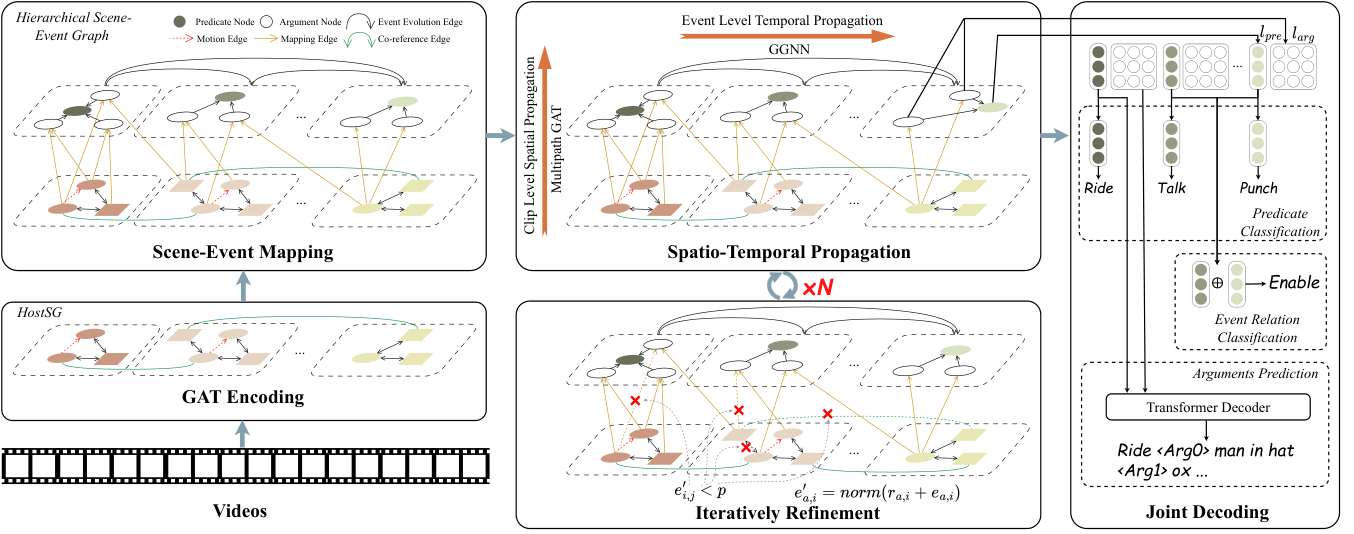
Built upon the HostSG, we then propose a nichetargeting VidSRL framework that performs total of five tiers of propagation (cf. Fig. 3). First, the HostSG of the input video is initialized by a graph attention model (GAT) (Velickovic et al. 2017) (cf. $\lx@sectionsign$ 5.1). Second, we expand the HostSG by dynamically generating new event nodes. Then we map the underlying scene structure to the high-level event semantic structure, by 1) creating edges between the object nodes in HostSG and the argument nodes in predicate-argument structure, and 2), connecting all the events along temporal dimensions, which results in an overall hierarchical scene-event graph (termed ICE) (cf. $\lx@sectionsign$ 5.2). Intuitively, the event actions of interest could only touch on part of visual objects in a scene; also some event arguments can associate with multiple visual objects simultaneously. Via such scene-event mapping, we bridge the gap between these two structures. Third, we perform the spatio-temporal propagation over the ICE graph, where a multipath-GAT encodes each TSG separately for the event spatial modeling, and a GRNN captures the overall event evolution and interrelations of the event-level structures along the temporal dimension (cf. $\lx@sectionsign$ 5.3). Fourth, we further propose iteratively refining the overall ICE structure via the Graph Information Bottleneck (GIB) technique (Wu et al. 2020), dynamically adjusting the object-argument mapping edges and the coreference edges such that the overall graph representation aligns with the end-task prediction and meanwhile screening the noisy structures (cf. $\lx@sectionsign$ 5.4). Fifth, after several iterations of structural refinement, we finally perform joint predictions for the three subtasks of VidSRL based on the well-updated ICE graph (cf. $\lx@sectionsign$ 5.5). Our end-to-end decoding scheme effectively avoids the error propagation introduced in the existing pipeline methods.

We perform experiments on the benchmark VidSRL data (Sadhu et al. 2021), where the results show that our framework significantly boosts the current state-of-the-art (SoTA) with 0.66~5.22 scores on several metrics. Further analyses demonstrate that the HostSG is effective in depicting the fine-grained spatial and temporal characteristics of video, and also the scene-event mapping mechanism is useful for bridging scene graph and event structure. We also reveal how the proposed iterative refinement optimizes the ICE structure and helps lead to better predictions.

2. Related Work

Semantic role labeling (SRL) is a fundamental task for revealing the underlying event semantics of given data. SRL is first pioneered in natural language processing (NLP) community, extracting the predicate-argument structure from given texts (Gildea and Jurafsky 2000; Xia et al. 2019; Fei et al. 2021a; Fei et al. 2021c; Fei et al. 2021b). SRL also shares much similarity in task definition with event extraction (Wan et al. 2023; Wu et al. 2023) and situation recognition (Yao et al. 2020; Cheng et al. 2022). Subsequently, the research of SRL is extended from text to vision modality, predicting the possible action labels and the corresponding argument expressions from image inputs (Wei et al. 2022; Cho et al. 2022). Compared with text-based SRL, visual SRL (or image situation recognition) is more challenging in requiring visual spatial semantics understanding (Gupta and Malik 2015; Yatskar et al. 2016). Later, cross-modal SRL is introduced, with both the texts and images as the input target for extracting the core predicate-argument structures (Zhang et al. 2017; Chiba and Higashinaka 2021). Multiple sources in different modalities intuitively provide complementary features and perspectives for better task understanding and prediction.

Recently, the SRL has been moved to the scenario of video modality, i.e., determining the semantic role and predicate structures given video (Sadhu et al. 2021). Essentially, video is naturally suitable for describing dynamic events, due to its characteristic of sequences of video frames. On the other hand, video understanding also raises challenges. Different from the static scenes in image modeling, video understanding is concerned with understanding both the spatial semantics and the temporal changes (Feichtenhofer et al. 2019; Dai et al. 2022; Geng et al. 2022; Wang et al. 2022a). Due to the difficulty of video modeling, VidSRL has received limited research attention (Sadhu et al. 2021; Khan et al. 2022; Yang et al. 2022a). For example, Sadhu et al. (2021) (Sadhu et al. 2021) pioneer the task of VidSRL by encoding the video with the vision Transformer model, where the coarse-grained visual understanding leads to significant spatial semantics loss. Khan et al. (2022) (Khan et al. 2022) model the VidSRL by further grounding the visual objects and entities across verb-role pairs. Yet, they still fail to consider the video temporality modeling. Very recently, Yang et al. (2022) (Yang et al. 2022a) propose tracking the object-level visual arguments so as to model the changes of states. In this regard, our work shares a similar spirit to (Yang et al. 2022a), but we differentiate theirs in three key aspects. First of all, we consider a more holistic and fine-grained video representation with the video scene graph structure, in which the fine-grained objects and their correlations, as well as the temporal dynamics all can be precisely modeled. Besides, our task formulation also considers the event relation subtask, sufficiently making use of the cross-event correlation features for better long-range dependence modeling. Third, we consider an end-to-end task paradigm, effectively reliving the error propagation in traditional pipeline modeling. In contrast, (Yang et al. 2022a) ignores the event relation prediction and also takes a cascade prediction of predicates and arguments.

This work also closely relates to the topic of scene graphs (SGs). An SG describes a given visual scene with a graph structure, where the fine-grained object nodes are connected with each other under certain relationships (Xu et al. 2017). Due to the semantic-level structured representation, SGs have been widely utilized for many downstream applications (Lu and Gao 2023; Chen et al. 2020). In this work, we consider the video SG, a.k.a., dynamic SG (DSG) (Haurilet et al. 2019; Li et al. 2022; Geng et al. 2021), or spatio-temporal SG (Cong et al. 2021; Ji et al. 2020), which is defined as representing each video frame with a static visual SG. However, with the raw video SG, maintaining an SG for all the frames can be much resource-consuming, and also results in redundant SG representations. Instead, we retrofit the video SG by merging the clip-level DSG into one single unified SG, where such renewal can effectively relieve the computational costs.

3. Task Formulation

Given a Video $V$ with $N$ clips $\{c_{i}\}_{i=1}^{N}$ , where each clips has the 2 seconds length without overlap and describes an event. VidSRL requires outputting $N$ related salient events $\{E_{i}\}_{i=1}^{N}$ corresponding to $N$ clips. Each event can be represented as:

(1)

\begin{split}e=\left\{v,\,\langle arg^{0},a^{0}\rangle,\,\langle arg^{1},a^{1}\rangle,\,...\right\},\end{split}

where $v\in\mathcal{V}$ denotes the salient event action, chosen from a pre-defined verb set $\mathcal{V}$ . $arg_{j}$ denotes the argument roles of $v$ , each of which is specified with a free text span $a_{j}$ . Each predicate has up to 10 arguments which is also predefined by VidSRL (Sadhu et al. 2021).

4. Holistic Spatio-temporal Scene Graph Construction

As cast earlier, we propose to construct a holistic spatio-temporal scene graph (HostSG) to model fine-grained object-level spatial and temporal characteristics of videos. The construction of HostSG is a three-step process, as shown in Fig. 2(a). First, we generate DSG for each video clip, containing several scene graphs. Then we merge each DSG (a set of static scene graphs) of a clip into an integrated graph, i.e., the temporalized DSG (TSG). Finally, we combine TSGs of all clips (each clip has one TSG) into the overall HostSG by adding cross-clip coreference edges.

Step-1: DSG Generation for Clip

We suppose the videos are already segmented into clips without overlap in timeline. We first perform keyframe extraction for each raw clip, so as to maintain the key semantics meanwhile reducing redundant features. To exactly capture the salient event content of the video clip and to avoid producing overlapping scene graphs from similar or blurry frames, we adopt a clustering-based extraction method (Song et al. 2016) to extract significant keyframes from the raw video clips. Then, these frames are fed into the scene graph parser MOTIFS-TDE (Tang et al. 2020) for producing the $DSG=\{G_{t}\}$ , consisting of a series of static scene graph $G_{t}=(V_{t},E_{t})$ of each keyframe of time $t\in T_{c}$ for clip $c$ . The scene graph parser outputs a probability score for each node, and only the top- $k$ ones will be selected for each $G_{t}$ .

Step-2: Merging DSG

Although we select the keyframes from the raw video clip, the resulting DSG of each clip can still contain many redundant nodes and edges that are unnecessary for computation and propagation (Wu et al. 2020). Also the DSG contains separate SG in sequence, where the temporal correlations are not explicitly modeled. Inspired by (Cherian et al. 2022), we combine the DSG of a clip into one temporalized Dynamic Scene Graph (TSG), representing both the spatial appearance information and the temporal object motions.

Concretely, according to the labels of the DSG object nodes, we divide all the objects into static and dynamic ones. The static nodes (e.g., house, street, trees) refer to the background objects that may not move observably within a short time, and the dynamic nodes (e.g., person, car, animal) are the opposite. We merge those static nodes across timeline based on their coreference, i.e., with highly identical categories and locations. Two static nodes $v_{t}\in G_{t},v_{t^{\prime}}\in G_{t^{\prime}}(t\neq t^{\prime})$ will be merged if they meet:

(2)

tag_{v_{t}}=tag_{v_{t^{\prime}}}\quad\text{and}\quad IoU(loc_{v_{t}},loc_{v_{t^{\prime}}})>d,

where $tag$ and $loc$ represent the label and bounding box of an object, and $IoU$ means the intersection over the union of two boxes. If a node has multiple candidate nodes in a frame, the one with the nearest centroid will be selected. After merging, we keep their original edges with other nodes. For dynamic nodes, instead of merging, we take the same way to recognize the coreference nodes but add edges between them to represent the motion relation. Then the DSG $\{G_{t}\}$ is compressed to a TSG $G^{tsg}_{c}=(V^{tsg}_{c},E^{tsg}_{c})$ for clip $c$ . The process is illustrated in Fig. 2(b).

Step-3: HostSG Construction

While a TSG depicts the inner-clip information, the cross-clip relations are still not well represented. To co-view all the clips holistically, we now combine the TSGs into one unified graph, by adding coreference edges between object nodes. However, due to the significant time interval between frames of different clips, there may be shot transitions or large movement of objects, which largely makes the IoU lose effectiveness. Here we instead link all TSGs by considering the semantic similarity between node visual features as well as their labels:

(3)

sim(v_{s},v_{o})=\text{Softmax}(Relu(h_{s}\cdot h_{o})),

where $h_{s},h_{s}$ denote the visual features of node $v_{s}\in V^{tsg}_{c},v_{o}\in V^{tsg}_{c^{\prime}}(c\neq c^{\prime})$ , respectively. Then we link the nodes meeting the following condition:

(4)

tag_{v_{s}}=tag_{v_{o}}\quad and\quad sim(v_{s},v_{o})>\gamma,

where $v_{s}$ and $v_{o}$ are from different TSGs. If a node has multiple candidate nodes in another frame to link, the candidate with maximum $sim$ is selected:

(5)

match(v_{s})=\mathop{argmax}_{v_{o^{\prime}}\in\{v|tag_{v}=tag{{}_{v_{s}}}\}}(sim(v_{s},v_{o^{\prime}})).

For dynamic nodes in a TSG, there can be multiple nodes representing one object. To tackle this, we treat all the dynamic nodes linked by motion edges as a whole, and average their representations for the similarity calculation:

(6)

sim(\bm{V}_{s},\bm{V}_{o})=\text{Softmax}(Relu(Avg(\bm{H}_{d})\cdot Avg(\bm{H}_{o}))),

where $\bm{V}_{s}$ and $\bm{V}_{o}$ are sets of dynamic nodes linked with motion edges. Once two sets of dynamic nodes are matched, we combine them by linking a node in one set with all the nodes in the other sets, producing a coreference cluster.

By traversing all the clip pairs with the above process, we can finally obtain the HostSG for the overall video. Here we denote the HostSG of a video as $\{G|(V,E)\}$ , where $V$ is the node set containing static nodes and dynamic nodes from all the TSGs, and $E$ is the edge set containing scene graph edges, motion edges and coreference edges. We provide more details of the HostSG construction in Appendix $\lx@sectionsign$ C.

5. VidSRL Framework

We propose a hierarchical framework to perform the VidSRL task. As shown in Fig. 3, the overall framework consists of five tiers: HostSG encoding, scene-event mapping, spatial-temporal propagation, iterative structure refinement and joint decoding.

5.1. HostSG Encoding

Given a HostSG $G$ of $N$ video clips, we denote the node representations of $G$ as $\bm{X}=\{x_{1},x_{2},...,x_{m}\}$ , where $x_{i}$ are initialized by the concatenation of the object visual features and the corresponding node label embeddings, both of which are obtained from a pre-trained scene graph parser, and a pre-trained language model encoder, respectively. Then a graph attention network (GAT) is used to encode $G$ :

(7)

\bm{X}_{host}=\mathop{\text{GAT}}_{\theta_{base}}(\bm{X}).

5.2. Scene-Event Mapping

An event structure consists of a predicate and several arguments, where the predicate reflects the event action and the arguments describe the related roles or modifiers. For instance, the structure of event-1 as in Fig. 1 contains a predicate “ride”, and three arguments, “man in hat”, “ox” and “slowly”. Such high-level event semantic structure does not well align with the low-level scene-based HostSG structure. Thus, in this step we aim to bridge the gap between these two structures. Technically, we connect the scene nodes of HostTSG and the event nodes of predicate-argument structure, leading to a broader structure of hierarchical scene-event graph (ICE).

As shown in Fig. 3, for each TSG $G^{tsg}$ in HostSG $G^{tsg}\subset G$ , we dynamically maintain a corresponding event structure $G^{evt}$ where the predicate node connects to all the argument nodes. In accordance with the VidSRL definition (Sadhu et al. 2021), we maintain 11 event nodes, including a predicate node, 5 real argument nodes, and 5 modifier argument nodes. Then, for each argument node $v_{e}$ in $G^{evt}$ , we tentatively link all object nodes in the corresponding TSG $G^{tsg}$ to $v_{e}$ , which will be further refined through training. Further, we create the edges between predicate nodes across all events, in which each predicate node directionally points to all the subsequent ones. Such cross-event connections help capture the event evolutionary relationships. The predicate node is initialized by averaging all the node representations of the TSG; while the argument nodes are initialized with the 10 argument embeddings:

(8)

\bm{X}_{evt}=\{\bm{x}_{p}=\text{Avg}\,(V^{tsg}),\bm{x}_{arg_{i}}=\text{Embed}(Arg_{i}),i\in[1,10]\}.

5.3. Spatio-Temporal Propagation

With the overall ICE graph, we now perform spatio-temporal propagation for a thorough feature learning. The message passing is divided into the spatial one at the clip level and the temporal one at the event level, subsequently.

Clip-level Spatial Propagation with Multipath-GAT

We encode the ICE graph at each clip dimension, which is the combination of the $G^{tsg}$ and $G^{evt}$ at the corresponding clip. Since we define multiple types of nodes and edges to represent various semantics, we consider a multipath-GAT for encoding, which keeps the information propagation separately among different types of nodes. Technically, based on the multi-head architecture of GAT, we divide these heads into three groups: coreference group, event group and normal group. The coreference group encodes only the object nodes of TSGs; the event group encodes only the abstract event nodes (i.e., predicate nodes and argument nodes) and the normal group encodes all the nodes:

(9)

\begin{split}\bm{H^{\prime}}_{host}=\mathop{\text{GAT}}&{}_{\theta_{obj}}(\bm{X}_{host}),\quad\bm{H^{\prime}}_{evt}=\mathop{\text{GAT}}_{\theta_{evt}}(\bm{X}_{evt}),\\ \bm{H^{\prime}}_{norm}&=\mathop{\text{GAT}}_{\theta_{norm}}([\bm{X}_{host},\bm{X}_{evt}]),\\ \end{split}

where $\bm{X}_{host}$ is the representation of object, obtained from the base scene graph encoder by Eq. (7). $\bm{X}_{evt}$ is obtained by Eq. (8). $\theta_{obj}$ , $\theta_{evt}$ and $\theta_{norm}$ are the three groups of GAT parameters. $\bm{H^{\prime}}_{obj}$ , $\bm{H^{\prime}}_{evt}$ and $\bm{H^{\prime}}_{norm}$ are the node representations of the final GAT layer. Next, we combine the three types of nodes with an element-wise summation:

(10)

\bm{H}=[\bm{H^{\prime}}_{host};\bm{H^{\prime}}_{evt}]+\bm{H^{\prime}}_{norm}.

Event-level Temporal Propagation with GGNN

By encoding the spatial features of each clip or event, we now process temporal information aggregation among events. Specifically, a Gated Graph Sequence Neural Network (GGNN) (Li et al. 2016) is adopted to propagate over all the event structures in ICE:

(11)

\bm{L}_{p}=\text{GGNN}(\bm{H}_{p}),

where $\bm{H}_{p}$ is the representations of predicate nodes obtained from $\bm{H}$ , and $\bm{L}_{p}$ is the final layer outputs of the GGNN.

5.4. Iterative Structural Refinement

At each end of the spatio-temporal propagation, we further perform structural refinement over the ICE structure. Previously, we build the fully-connected initial edges of argument-object mapping, while the realistic case can be that one argument may also associate with a very small part of the objects in scenes. Also the initial structures in terms of the event evolution edges as well as the coreference edges among TSGs should also be updated to best meet the task prediction. To this end, we iteratively adjust the overall structure. Each refinement step is processed after one GAT layer.

Table 1. Main results on the VidSRL dataset. “Verb Cls”, “SRL” and “EvtRel” represents the three subtasks verb classification, semantic role labeling and event relation prediction. The CIDEr score is also computed over every verb-sense (CIDEr-Verb) and over argument-types (CIDEr-Arg). Bold numbers are the best, and underlined ones are the second best. Our results are averaged on five running with different seeds. Gray color: methods use ground-truth verb annotations for SRL training.

$\bullet$ Pipeline
		Verb Cls			SRL						EvRel
		Acc@1(%)	Acc@5(%)	Rec@5(%)	CIDEr	Rouge-L	CIDEr-Vb	CIDEr-Arg	Lea	Lea-S	Macro-Acc(%)
	VidSitu-GPT2 (Sadhu et al. 2021)	-	-	-	34.67	40.08	42.97	34.45	48.08	28.10	-
	VidSitu-I3D (Sadhu et al. 2021)	30.17	66.83	4.88	47.06	42.41	51.67	42.76	48.92	33.58	-
	VidSitu-SlowFast (Sadhu et al. 2021)	32.64	69.20	6.11	45.52	42.66	55.47	42.82	50.48	31.99	34.13
$\bullet$ Joint
	VidSitu-e2e (Yang et al. 2022a)	46.79	75.90	23.38	30.33	29.98	39.56	23.97	35.92	-	-
	OME (Yang et al. 2022a)	52.75	83.88	28.44	47.82	40.91	54.51	44.32	-	-	-
	OME(disp) (Yang et al. 2022a)	53.32	84.00	28.61	48.46	41.89	56.04	44.60	-	-	-
	OME(disp)+OIE (Yang et al. 2022a)	53.36	83.94	28.72	47.16	40.86	53.96	42.78	-	-	-
	VideoWhisperer (Khan et al. 2022)	45.06	75.59	25.25	52.30	35.84	61.77	38.18	38.00	-	-
	HostSG (Ours)	56.15	86.33	29.38	55.09	43.13	64.24	47.68	55.70	35.01	35.97
		(+2.79)	(+2.33)	(+0.66)	(+2.79)	(+1.24)	(+2.47)	(+3.08)	(+5.22)	(+3.2)	(+1.84)

Edge weights adjustment

We refine the graph structure via adjusting the edge weights. The ICE has five types of edge, i.e., DSG edges, coreference edges, scene-event mapping edges, predicate-argument edges and event evolution edges. The predicate-argument edges are fixed due to the inherent event structure, and we adjust the other four types. We first calculate a relation score $r_{a,i}$ between a pair of nodes $a$ and $i$ :

(12)

\begin{split}\bm{a}_{a,i}&=\frac{\exp{(\bm{W_{1}}[\bm{h}_{a};\bm{h}_{i}])}}{\sum_{j\in\Phi}\exp{(\bm{W_{1}}[\bm{h}_{a};\bm{h}_{j}])}},\\ r_{a,i}&=Softmax(FFN(\bm{a}_{a,i})),\end{split}

where $\bm{h}_{a}$ and $\bm{h}_{i}$ are the hidden representations of node $a$ and $i$ , $\Phi$ denotes the set of all nodes in ICE. $\bm{W_{1}}$ and $\bm{W_{2}}$ are learnable parameters. Then we change the weight of edge $e_{a,i}$ to:

(13)

e^{\prime}_{a,i}=\text{norm}(r_{a,i}\cdot e_{a,i}).

Afterwards, we filter the edges with low $e^{\prime}_{a,i}$ by setting its weight to 0. Specifically, we further cut the coreference edges between nodes with different labels due to the natural constraint. Through edge adjustment, the model will adaptively filter noisy edges (setting weights to 0) and meanwhile newly add informative edges (setting weights to non-zero).

Assistant optimization

Thereafter, we obtain an adjusted ICE from the final layer refinement, i.e., $G^{-}$ , and its node representations $\bm{H}^{-}$ . We perform pooling over $\bm{H}$ to obtain the graph representation $\bm{g}$ and further concatenate it with predicate nodes as the context features for event verb and event pair relation:

(14)

\begin{split}\bm{a}_{v}=[\bm{g};\bm{h}^{-}],\quad\bm{a}_{rel}=[\bm{g};\bm{h}^{-}_{i};\bm{h}^{-}_{j}],\end{split}

where $\bm{h}\in\bm{H^{-}}$ is the representation of the predicate node.

To ensure the adjusted coreference edges and mapping edges are informative enough, we consider an assistant optimization objectives. Inspired by (Wu et al. 2020), we denote $\bm{z}_{a},\bm{z}_{rel}$ as the compact information of the resulting $G^{-}$ , which is sampled from a Gaussian distribution parameterized by $\bm{a}_{v}$ and $\bm{a}_{rel}$ . The we adopt the GIB-driven loss:

(15)

\mathcal{L}_{GIB}=\min[-I(\bm{z}_{v},Y_{v})-I(\bm{z}_{rel},Y_{rel})+I(\bm{z}_{v},G)+I(\bm{z}_{rel},G)],

where $I(\cdot)$ denotes the mutual information. In appendix $\lx@sectionsign$ A, we give the detailed technical process of GIB optimization.

5.5. Joint Task Decoding

In the decoding stage, we use three heads for the three subtasks of VidSRL separately. For verb prediction and event relation classification, we use the MLP classifiers respectively.

(16)

\begin{split}\bm{v}_{i}=\mathop{\text{MLP}}_{verb}(\bm{l}_{p_{i}}),\quad\bm{r}(i\rightarrow j)=\mathop{\text{MLP}}_{evtrel}([\bm{l}_{p_{i}};\bm{l}_{p_{j}}]),\end{split}

where $\bm{l}_{p_{i}},\bm{l}_{p_{j}}\in\bm{L}_{p}$ is the predicate node representation of event $i$ . $v_{i}$ and $r(i\rightarrow j)$ are further passed through a softmax function and predict the verb for event $e$ and the event relation from event $i$ to event $j$ .

For argument generation, we adopt a transformer decoder to generate the arguments in a sequence-to-sequence manner. Different from (Sadhu et al. 2021), we passed argument node features as the input token embeddings:

(17)

args=\text{TextDecoder}(\bm{l}_{p_{i}},\bm{h}_{arg_{1}},\bm{h}_{arg_{2}},...\bm{h}_{arg_{10}}),

where $\bm{h}_{arg_{i}}\in\bm{H}$ is the argument node representation.

5.6. Training Objectives

For the three subtasks of VidSRL, i.e., verb prediction, event relation prediction and arguments generation, we use cross-entropy between decoder outputs and the ground-truth as the objectives, denoted by $\mathcal{L}_{v}$ , $\mathcal{L}_{r}$ and $\mathcal{L}_{arg}$ . Based on the objectives of the three subtasks and the assistant GIB loss of graph refinement, we set the final joint loss as:

(18)

\mathcal{L}=\mathcal{L}_{v}+\eta_{1}\mathcal{L}_{r}+\eta_{2}\mathcal{L}_{arg}+\eta_{3}\mathcal{L}_{GIB}.

6. Experiments

6.1. Settings

We experiment with the VidSRL data (Sadhu et al. 2021), which contains 28K videos from movies. Each video is 10 seconds in length, and is cut into five clips with 2 seconds each. VidSRL annotations contain 2K+ verb categories with more than three arguments (semantic roles) each. For fair comparison, we follow (Sadhu et al. 2021) to measure verb prediction with Acc@K and Recall@K, and use top-1 accuracy for event relation classification. For free-form argument generation, we follow (Sadhu et al. 2021) to measure the prediction of ARG0, ARG₁, ARG₂, ARG_LOC and ARG_SCENE, using CIDEr, ROUGE-L to measure agreement computation and Lea (Moosavi and Strube 2016) to measure coreferencing capability. We compare our model with recent SoTA methods with different architectures. We divide all the methods to 1) pipeline and the 2) joint ones, where the pipeline methods train modules for the three VidSRL tasks separately, while the joint methods train one model jointly. The pipeline methods may use the golden-standard verb-role pairs as inputs for SRL subtask, while the joint methods train the three tasks together with only videos as inputs. For DSG parsing, we extract 5 key frames from each clips, and adopt MOTIFS-TD (Tang et al. 2020) to get the scene graphs and keep the top 15 objects. We follow (Cherian et al. 2022) for dividing static and dynamic nodes when merging the DSGs. Model hyperparameters and more detailed experiment settings are shown in Appendix $\lx@sectionsign$ B.

6.2. Main Results

Table 1 shows the overall results. Overall, the new proposed joint models outperform the baseline pipeline methods. For the verb classification task, we can see the joint models with far better features achieve significant improvements than the baselines with only I3D and SlowFast features. Note that the “VidSitu-GPT2” line means it only uses a visual-blind language model to predict arguments with the textual inputs of verbs. Thus it has no results for verb and event relation prediction. “VidSitu-GPT2” only achieves a very low performance due to the missing of video information.

For SRL subtask, the results of pipelines take advantage of the ground-truth annotations of verbs by teacher-forcing thus we mark them with the gray color. Instead, we report the reproduced results of (Khan et al. 2022) in “VidSitu-e2e” for a fair comparison. We can see the “OME” and “VideoWhisperer” models achieve remarked progress from “VidSitu-e2e”. In contrast, our proposed method achieves significantly better results over three tasks on all metrics, demonstrating its efficacy. Furthermore, our model could cover the event relation prediction task while most other models do not.

Table 2. Module ablation results. ‘w/o SG features’ means ablating the graph modeling of scene graph feature, while instead using the overall video features. ‘w/o SG-Evt mapping’ means replacing the generated event nodes with the average pooling of the object nodes features. ‘w/o Refinement’ means ablating the iterative refinement. ‘w/o Multipath GAT’ means replacing the multipath GAT with a normal GAT. ‘Base-GAT’ and ‘GGNN’ represents the base encoder and the GGNN network before decoder.

	Acc@1	CIDEr	Macro-Acc
HostSG (Full)	56.15	55.09	35.97
w/o SG features	46.19(-9.96)	47.38(-7.71)	34.40(-1.57)
w/o SG-Evt mapping	53.43(-2.72)	52.38(-2.71)	34.81(-1.16)
w/o Refinement	54.51(-1.64)	52.85(-2.24)	35.06(-0.91)
w/o Multipath GAT	54.92(-1.23)	53.35(-1.74)	35.50(-0.47)
w/o Base-GAT	55.10(-1.05)	54.93(-0.96)	35.83(-0.16)
w/o GGNN	55.77(-0.38)	55.01(-0.08)	35.00(-0.97)

Model Ablation. Now we quantify the contribution of each design in our systems via model ablation, as shown in Table 2. First, we can see that the scene graph features give the biggest influence, contributing 9.96 Acc for verb classification, 7.71 CIDEr for argument prediction and 1.57 for event relation classification. Besides, the scene-event mapping and the refinement mechanism also play an essential role in our framework. The GGNN mainly contributes to the event relation classification tasks, gaining 0.97 Acc. Other module designs, the base GAT and multipath-GAT, enhance the system more or less.

6.3. Analysis and Discussion

$\blacktriangleright$ Q1: Does HostSG provide informative spatial and temporal features for VidSRL? The primary motivation of our method is that the HostSG could provide fine-grained spatial and temporal features. We now downgrade the HostSG with the object features without a graph structure, and replace $\bm{X}_{host}$ with the raw object features, keeping the event nodes in ICE. As shown in Figure 4, the modeling with object features decreases the performance markedly.

We also explore the temporal modeling of inner-clip DSG merging. When extracting frames, we try 11, 5 and 1 frames for each clip separately. When the number of frames decays to 1, there is no temporal information then. As shown in Table 3, single frames without temporal information abate final performance, while the situations on 5 or 11 frames have consistent performance. We suppose that for a 2s clip, five keyframes are enough to capture the salient objects from different temporal scenes. Too many frames may bring noisy information, while single frame may lose some objects due to the potential scene transition.

Table 3. Influence of different numbers of frame extraction. ‘w/o Key Frame Extraction’ means we extract frames with a constant interval.

Acc@1	CIDEr	Macro-Acc
$\bullet$ 1 Frame/Clip	41.48	36.85	33.91
w/o Key Frame Extraction	41.51	37.10	34.02
$\bullet$ 5 Frames/Clip	56.15	55.09	35.97
w/o Key Frame Extraction	56.13	54.77	35.16
$\bullet$ 11 Frames/Clip	55.15	54.72	35.31
w/o Key Frame Extraction	55.04	54.67	35.29

Figure 4. Comparison between the results of scene graph features and object features.

Figure 5. Comparison between the results of HostSG with and without cross-clip coreference edges.

$\blacktriangleright$ Q2: How does the cross-clip coreference information aid the task? Next, we consider investigating the influence of coreference information. We cut all the cross-clip coreference edges of HostSG for comparison and keep the remaining structure, and then we can get the perception of its necessity. The results are shown in Figure 5, the HostSG without cross-clip coreference decreases the performance by a noticeable margin. We further provide a qualitative analysis to explore whether it correctly models the cross-clip coreference relations. We consider the weights of cross-clip edges after the final layer. As shown in Figure 6, we can see the weights gather among the object nodes in a coreference cluster.

$\blacktriangleright$ Q3: Does the scene-event mapping mechanism really bridge the scene-event gap? Overall, as shown in Table 2, the scene-event mapping contributes significantly to the final performance, gaining 2.72 Acc@1 2.71 CIDEr and 1.16 Macro-Acc than the model with only HostSG features. We can further empirically analyze the scene-event mapping via an example in Figure 8. In this case, the ICE graph structure reflects the scene-event mapping results. In event 1, the model with only HostSG feature can not capture the cross-event object tie which is not presented in its own clip while the model with mapping does. Furthermore, the model with only HostSG fails to predict the right predicate for event 3 by cross-event information (the state in event 2). The case clearly demonstrates the effectiveness of the scene-event mapping mechanism.

Figure 7. The trends of changing amplitude of edge weights (average of all adjusted edges), along with task performance.

$\blacktriangleright$ Q4: Can iterative refinement really denoise the edges? First, we plot the trajectories of edge-adjusting amplitudes through training steps, along with the trends of task performance. As shown in Figure 7, the weight variability of edges decreases gradually while the task performance climbs along with the training process. The chart shows that the edge refinement indeed optimizes the graph structure by adjusting edge weights.

$\blacktriangleright$ Q5: Impact of the temporalized dynamic scene graph. In realistic scenarios, we expect to model each object in each frame for video understanding. But in practice, there are too many redundant objects in frames with a high sampling rate, which will cause extreme computational costs. The proposed temporalized dynamic scene graph could compress the DSG by merging the static nodes. We could assume that their slight movement in a short clip will not change their semantics. This is reasonable because most static objects in a video scene provide little information to understand the salient event. Table 4 gives the comparison between a model with TSG and raw DSG, where the performance in the two situations is consistent. That means the static node merging does not lose key information. We can also find how the object number affects the performance. The results show that the fewer objects may lose some information while the redundant objects may bring noisy information.

Table 4. Comparison between TSG and raw DSG without node merging, which means we treat all the DSG nodes as dynamic nodes. “Obj Num” means keep top N objects when parsing the scene graph.

	Obj Num	Acc@1	CIDEr	Macro-Acc
Raw DSG	5	54.19	53.03	34.91
	15	56.21	55.10	35.88
	20	55.53	54.91	34.80
TSG	5	54.31	52.77	34.66
	15	56.15	55.09	35.97
	20	55.38	54.20	35.47

7. Conclusions

In this paper, we introduce a novel approach to the challenging VidSRL task. Our approach involves modeling the fine-grained spatial semantics and temporal dynamics of videos by constructing a holistic spatio-temporal scene graph representation. We devise a scene-event mapping mechanism to bridge the gap between the underlying scene structure and the high-level event semantic structure. Furthermore, we propose an iterative structure refinement strategy to enhance the compatibility between the graph representations and VidSRL reasoning. The proposed framework enables us to jointly predict the three subtasks of VidSRL, which effectively avoids the error propagation issue in the current pipeline paradigm. Empirical evaluations on the benchmark dataset demonstrate that our approach outperforms current methods.

References

(1)
Cai et al. (2022) Desheng Cai, Shengsheng Qian, Quan Fang, Jun Hu, and Changsheng Xu. 2022. Adaptive Anti-Bottleneck Multi-Modal Graph Learning Network for Personalized Micro-video Recommendation. In Proceedings of ACM MM 2022. 581–590.
Cao et al. (2020) Da Cao, Yawen Zeng, Xiaochi Wei, Liqiang Nie, Richang Hong, and Zheng Qin. 2020. Adversarial Video Moment Retrieval by Jointly Modeling Ranking and Localization. In Proceedings of ACM MM 2020. ACM, 898–906.
Chen et al. (2020) Shizhe Chen, Qin Jin, Peng Wang, and Qi Wu. 2020. Say As You Wish: Fine-Grained Control of Image Caption Generation With Abstract Scene Graphs. In Proceedings of CVPR 2020. 9959–9968.
Cheng et al. (2022) Zhi-Qi Cheng, Qi Dai, Siyao Li, Teruko Mitamura, and Alexander Hauptmann. 2022. GSRFormer: Grounded Situation Recognition Transformer with Alternate Semantic Attention Refinement. In Proceedings of MM 2022. 3272–3281.
Cherian et al. (2022) Anoop Cherian, Chiori Hori, Tim K Marks, and Jonathan Le Roux. 2022. (2.5+ 1) D Spatio-Temporal Scene Graphs for Video Question Answering. In Proceedings of AAAI 2022, Vol. 36. 444–453.
Chiba and Higashinaka (2021) Yuya Chiba and Ryuichiro Higashinaka. 2021. Dialogue Situation Recognition for Everyday Conversation Using Multimodal Information. In Proceedings of Interspeech 2021. 241–245.
Cho et al. (2022) Junhyeong Cho, Youngseok Yoon, and Suha Kwak. 2022. Collaborative Transformers for Grounded Situation Recognition. In Proceedings of CVPR 2022. 19627–19636.
Cong et al. (2021) Yuren Cong, Wentong Liao, Hanno Ackermann, Bodo Rosenhahn, and Michael Ying Yang. 2021. Spatial-Temporal Transformer for Dynamic Scene Graph Generation. In Proceedings of ICCV 2021. 16352–16362.
Dai et al. (2022) Peng Dai, Xin Yu, Lan Ma, Baoheng Zhang, Jia Li, Wenbo Li, Jiajun Shen, and Xiaojuan Qi. 2022. Video Demoiréing with Relation-Based Temporal Consistency. In Proceedings of CVPR 2022. 17601–17610.
Fei et al. (2021a) Hao Fei, Fei Li, Bobo Li, and Donghong Ji. 2021a. Encoder-Decoder Based Unified Semantic Role Labeling with Label-Aware Syntax. In Proceedings of the AAAI Conference on Artificial Intelligence. 12794–12802.
Fei et al. (2021b) Hao Fei, Shengqiong Wu, Yafeng Ren, Fei Li, and Donghong Ji. 2021b. Better Combine Them Together! Integrating Syntactic Constituency and Dependency Representations for Semantic Role Labeling. In Findings of the Association for Computational Linguistics: ACL/IJCNLP 2021. 549–559.
Fei et al. (2021c) Hao Fei, Meishan Zhang, Bobo Li, and Donghong Ji. 2021c. End-to-end Semantic Role Labeling with Neural Transition-based Model. In Proceedings of the AAAI Conference on Artificial Intelligence. 12803–12811.
Feichtenhofer et al. (2019) Christoph Feichtenhofer, Haoqi Fan, Jitendra Malik, and Kaiming He. 2019. SlowFast Networks for Video Recognition. In Proceedings of ICCV 2019. 6201–6210.
Feng et al. (2021) Shengyu Feng, Subarna Tripathi, Hesham Mostafa, Marcel Nassar, and Somdeb Majumdar. 2021. Exploiting Long-Term Dependencies for Generating Dynamic Scene Graphs. CoRR abs/2112.09828 (2021). arXiv:2112.09828
Geng et al. (2021) Shijie Geng, Peng Gao, Moitreya Chatterjee, Chiori Hori, Jonathan Le Roux, Yongfeng Zhang, Hongsheng Li, and Anoop Cherian. 2021. Dynamic Graph Representation Learning for Video Dialog via Multi-Modal Shuffled Transformers. In Proceedings of AAAI 2021. 1415–1423.
Geng et al. (2022) Zhicheng Geng, Luming Liang, Tianyu Ding, and Ilya Zharkov. 2022. RSTT: Real-time Spatial Temporal Transformer for Space-Time Video Super-Resolution. In Proceedings of CVPR 2022. 17420–17430.
Gildea and Jurafsky (2000) Daniel Gildea and Daniel Jurafsky. 2000. Automatic Labeling of Semantic Roles. In Proceedings of ACL 2000. 512–520.
Gupta and Malik (2015) Saurabh Gupta and Jitendra Malik. 2015. CoRR abs/1505.04474 (2015). arXiv:1505.04474
Haurilet et al. (2019) Monica Haurilet, Ziad Al-Halah, and Rainer Stiefelhagen. 2019. DynGraph: Visual Question Answering via Dynamic Scene Graphs. In Proceedings of GCPR 2019 (Lecture Notes in Computer Science, Vol. 11824). 428–441.
Ji et al. (2020) Jingwei Ji, Ranjay Krishna, Li Fei-Fei, and Juan Carlos Niebles. 2020. Action Genome: Actions As Compositions of Spatio-Temporal Scene Graphs. In Proceedings of CVPR 2020. 10233–10244.
Ji et al. (2021) Jiayi Ji, Yunpeng Luo, Xiaoshuai Sun, Fuhai Chen, Gen Luo, Yongjian Wu, Yue Gao, and Rongrong Ji. 2021. Improving image captioning by leveraging intra- and inter-layer global representation in transformer network. In Proceedings of the AAAI Conference on Artificial Intelligence. 1655–1663.
Ji et al. (2022) Jiayi Ji, Yiwei Ma, Xiaoshuai Sun, Yiyi Zhou, Yongjian Wu, and Rongrong Ji. 2022. Knowing what to learn: a metric-oriented focal mechanism for image captioning. IEEE Transactions on Image Processing 31 (2022), 4321–4335.
Kang and Han (2023) Soo-Han Kang and Ji-Hyeong Han. 2023. Video Captioning Based on Both Egocentric and Exocentric Views of Robot Vision for Human-Robot Interaction. Int. J. Soc. Robotics 15, 4 (2023), 631–641.
Khan et al. (2022) Zeeshan Khan, C. V. Jawahar, and Makarand Tapaswi. 2022. Grounded Video Situation Recognition. In Proceedings of NeurIPS 2022.
Li et al. (2016) Yujia Li, Daniel Tarlow, Marc Brockschmidt, and Richard S. Zemel. 2016. Gated Graph Sequence Neural Networks. In Proceedings of ICLR 2016.
Li et al. (2022) Yiming Li, Xiaoshan Yang, and Changsheng Xu. 2022. Dynamic Scene Graph Generation via Anticipatory Pre-training. In Proceedings of CVPR. 13864–13873.
Lu and Gao (2023) Xuyang Lu and Yang Gao. 2023. Guide and interact: scene-graph based generation and control of video captions. Multim. Syst. 29, 2 (2023), 797–809.
Luo et al. (2021) Yunpeng Luo, Jiayi Ji, Xiaoshuai Sun, Liujuan Cao, Yongjian Wu, Feiyue Huang, Chia-Wen Lin, and Rongrong Ji. 2021. Dual-level collaborative transformer for image captioning. In Proceedings of the AAAI Conference on Artificial Intelligence. 2286–2293.
Moosavi and Strube (2016) Nafise Sadat Moosavi and Michael Strube. 2016. Which Coreference Evaluation Metric Do You Trust? A Proposal for a Link-based Entity Aware Metric. In Proceedings of ACL 2016.
Nag et al. (2023) Sayak Nag, Kyle Min, Subarna Tripathi, and Amit K. Roy-Chowdhury. 2023. Unbiased Scene Graph Generation in Videos. CoRR abs/2304.00733 (2023). arXiv:2304.00733
Nie et al. (2022) Liqiang Nie, Leigang Qu, Dai Meng, Min Zhang, Qi Tian, and Alberto Del Bimbo. 2022. Search-oriented Micro-video Captioning. In Proceedings of ACM MM 2022. 3234–3243.
Sadhu et al. (2021) Arka Sadhu, Tanmay Gupta, Mark Yatskar, Ram Nevatia, and Aniruddha Kembhavi. 2021. Visual Semantic Role Labeling for Video Understanding. In Proceedings of CVPR. 5589–5600.
Song et al. (2016) Yale Song, Miriam Redi, Jordi Vallmitjana, and Alejandro Jaimes. 2016. To click or not to click: Automatic selection of beautiful thumbnails from videos. In Proceedings of ACM MM 2016. 659–668.
Tang et al. (2020) Kaihua Tang, Yulei Niu, Jianqiang Huang, Jiaxin Shi, and Hanwang Zhang. 2020. Unbiased Scene Graph Generation From Biased Training. In Proceedings of CVPR 2020. 3713–3722.
Velickovic et al. (2017) Petar Velickovic, Guillem Cucurull, Arantxa Casanova, Adriana Romero, Pietro Liò, and Yoshua Bengio. 2017. Graph Attention Networks. CoRR abs/1710.10903 (2017).
Wan et al. (2023) Qizhi Wan, Changxuan Wan, Keli Xiao, Rong Hu, and Dexi Liu. 2023. A Multi-channel Hierarchical Graph Attention Network for Open Event Extraction. ACM Trans. Inf. Syst. 41, 1 (2023), 20:1–20:27.
Wang et al. (2023b) Chenwei Wang, Siyi Luo, Jifang Pei, Xiaoyu Liu, Yulin Huang, Yin Zhang, and Jianyu Yang. 2023b. An Entropy-Awareness Meta-Learning Method for SAR Open-Set ATR. IEEE Geoscience and Remote Sensing Letters (2023).
Wang et al. (2023c) Chenwei Wang, Jifang Pei, Siyi Luo, Weibo Huo, Yulin Huang, Yin Zhang, and Jianyu Yang. 2023c. SAR Ship Target Recognition via Multiscale Feature Attention and Adaptive-Weighed Classifier. IEEE Geoscience and Remote Sensing Letters 20 (2023), 1–5.
Wang et al. (2022b) Chenwei Wang, Jifang Pei, Jianyu Yang, Xiaoyu Liu, Yulin Huang, and Deqing Mao. 2022b. Recognition in Label and Discrimination in Feature: A Hierarchically Designed Lightweight Method for Limited Data in SAR ATR. IEEE Transactions on Geoscience and Remote Sensing 60 (2022), 1–13.
Wang et al. (2023a) Haowei Wang, Jiayi Ji, Yiyi Zhou, Yongjian Wu, and Xiaoshuai Sun. 2023a. Towards Real-Time Panoptic Narrative Grounding by an End-to-End Grounding Network. Proceedings of the AAAI Conference on Artificial Intelligence (2023), 2528–2536.
Wang et al. (2022a) Jue Wang, Gedas Bertasius, Du Tran, and Lorenzo Torresani. 2022a. Long-Short Temporal Contrastive Learning of Video Transformers. In Proceedings of CVPR 2022. 13990–14000.
Wei et al. (2022) Meng Wei, Long Chen, Wei Ji, Xiaoyu Yue, and Tat-Seng Chua. 2022. Rethinking the Two-Stage Framework for Grounded Situation Recognition. In Proceedings of AAAI 2022. 2651–2658.
Wu et al. (2023) Mengjie Wu, Maofu Liu, Luyao Wang, and Huijun Hu. 2023. A Chinese Fine-grained Financial Event Extraction Dataset. In Proceedings of WWW 2023. 1229–1235.
Wu et al. (2020) Tailin Wu, Hongyu Ren, Pan Li, and Jure Leskovec. 2020. Graph information bottleneck. In Proceedings of NeurIPS 2020, Vol. 33. 20437–20448.
Xia et al. (2019) Qingrong Xia, Zhenghua Li, and Min Zhang. 2019. A Syntax-aware Multi-task Learning Framework for Chinese Semantic Role Labeling. In Proceedings of EMNLP-IJCNLP 2019. 5381–5391.
Xu et al. (2017) Danfei Xu, Yuke Zhu, Christopher B. Choy, and Li Fei-Fei. 2017. Scene Graph Generation by Iterative Message Passing. In Proceedings of CVPR 2017. 3097–3106.
Yang et al. (2022a) Guang Yang, Manling Li, Jiajie Zhang, Xudong Lin, Shih-Fu Chang, and Heng Ji. 2022a. Video Event Extraction via Tracking Visual States of Arguments. In Proceedings of AAAI 2020.
Yang et al. (2022b) Xu Yang, Hanwang Zhang, and Jianfei Cai. 2022b. Auto-Encoding and Distilling Scene Graphs for Image Captioning. IEEE Trans. Pattern Anal. Mach. Intell. 44, 5 (2022), 2313–2327.
Yao et al. (2020) Wenlin Yao, Cheng Zhang, Shiva Saravanan, Ruihong Huang, and Ali Mostafavi. 2020. Weakly-Supervised Fine-Grained Event Recognition on Social Media Texts for Disaster Management. In Proceedings of AAAI 2020. 532–539.
Yatskar et al. (2016) Mark Yatskar, Luke S. Zettlemoyer, and Ali Farhadi. 2016. Situation Recognition: Visual Semantic Role Labeling for Image Understanding. In Proceedings of CVPR. 5534–5542.
Zhang et al. (2017) Tongtao Zhang, Spencer Whitehead, Hanwang Zhang, Hongzhi Li, Joseph G. Ellis, Lifu Huang, Wei Liu, Heng Ji, and Shih-Fu Chang. 2017. Improving Event Extraction via Multimodal Integration. In Proceedings of ACM MM 2017. 270–278.

Appendix A Detailed GIB-guided Assistant Optimization

Here, we provide more background information about the graph information bottleneck (GIB) principle. Given the original graph G, and the target Y, the goal of representation learning is to obtain the refined graph $G^{-}$ which is maximally informative w.r.t Y:

(19)

\min_{G^{-}}[-I(G^{-},Y)+\beta I(G^{-},G)],

where $I(G^{-},G)$ minimizes the mutual information between $G$ and $G^{-}$ such that $G^{-}$ learns to be the minimal and compact one of $G$ . $I(G^{-},Y)$ is the prediction objective, which encourages $G^{-}$ to be informative enough to predict the label $Y$ . $\beta$ is a Lagrangian coefficient. For our HostSG, we denote $\bm{z}$ as the compact information of the resulting $G^{-}$ , which is sampled from a Gaussian distribution parameterized by $\bm{a}_{v}$ and $\bm{a}_{rel}$ , which are obtained by Eq. (14). The the Eq. 19 can be rephrased as:

(20)

\mathcal{L}_{GIB}=\min[-I(\bm{z}_{v},Y_{v})-I(\bm{z}_{rel},Y_{rel})+I(\bm{z}_{v},G)+I(\bm{z}_{rel},G)],

where $Y_{v}$ and $Y_{rel}$ are the labels of verb prediction and event relation prediction. The term $-I(\bm{z}_{v},Y_{v})$ and $-I(\bm{z}_{rel},Y_{rel})$ can be expanded as:

(21)

\begin{split}-I(\bm{z}_{v},Y_{v})&\leq-\int p(Y_{v},\bm{z}_{v})\log q(Y_{v}|\bm{z}_{v})dY_{v}d\bm{z}_{v}+H(Y_{v})\\ &:=\mathcal{L}_{CE}(q(Y_{v}|\bm{z}_{v}),Y_{v}),\\ -I(\bm{z}_{rel},Y_{rel})&\leq-\int p(Y_{rel},\bm{z}_{rel})\log q(Y_{rel}|\bm{z}_{rel})dYd\bm{z}+H(Y_{rel})\\ &:=\mathcal{L}_{CE}(q(Y_{rel}|\bm{z}_{rel}),Y_{rel}),\end{split}

where $q(Y_{v}|\bm{z}_{v})$ and $q(Y_{rel}|\bm{z}_{rel})$ are variational approximation of the true posterior $p(Y_{v}|\bm{z}_{v})$ and $p(Y_{rel}|\bm{z}_{rel})$ . For $I(\bm{z}_{v},G)$ and $I(\bm{z}_{rel},G)$ , we estimate their upper bound via reparameterization trick:

(22)

\begin{split}I(\bm{z}_{v},G)&\leq\int p(\bm{z}_{v}|G)\log\frac{p(\bm{z}_{v}|G)}{r(\bm{z}_{v})}d\bm{z}dG\\ &:=\text{KL}(p(\bm{z}_{v}|G)||r(\bm{z}_{v})),\\ I(\bm{z}_{rel},G)&\leq\int p(\bm{z}_{rel}|G)\log\frac{p(\bm{z}_{rel}|G)}{r(\bm{z})}d\bm{z}dG\\ &:=\text{KL}(p(\bm{z}_{rel}|G)||r(\bm{z}_{rel})),\end{split}

Appendix B Detailed Implementation Settings

Table 5. Model hyperparameters.

Hyper-param.	Value
dimension of ROI feature	2048
dimension of Transformer hiddens	1024
dimention of GAT hiddens	1024
dimention of GGNN hiddens	1024
layer number of GAT	3
refinement times each batch	2
max object number	15
IoU threshold $d$	0.5
similarity threshold $\gamma$	0.3
S $3$ cutting threshold $p_{cut}$	0.1
max text length	80
optimizer	Adam
dropout	0.1
learning rate	1e-4
bach size	16
epoch	20
beam search number	5

A summary of the hyperparameter choice is shown in Table 5

Appendix C Model Details

Table 6. Static and dynamic objects.

Type	Object Labels
static object	bed,bag, banana, basket, beach, bench, board, bottle, bowl, box, branch, building, cabinet, chair, clock, counter, cup, curtain, desk, door, drawer, fence, flag, flower, food, fork, fruit, glass, handle, hill, house, lamp, laptop, leaf, letter, light, logo, mountain, number, orange, paper, phone, pillow, pizza, plant, plate, pole, post, pot, racket, railing, rock, roof, room, screen, seat, shelf, sidewalk, sign, sink, skateboard, ski, snow, stand, street, surfboard, table, tile, tire, toilet, towel, tower, track, tree, trunk, umbrella, vase, vegetable, window, windshield, wire
dynamic object	airplane, arm, animal, bear, bird, bike, boat, boot, boy, bus, cap, car, cat, child, coat, cow, dog, ear, elephant, engine, eye, face, finger, girl, giraffe, glove, guy, hair, hand, hat, head, helmet, horse, jacket, jean, kid, kite, lady, leg, man, men, motorcycle, mouth, neck, nose, pant, paw, people, person, plane, player, sheep, shirt, shoe, short, skier, sneaker, sock, tail, tie, train, truck, vehicle, wave, wheel, wing, woman, zebra

Type

Object Labels

static object

bed,bag, banana, basket, beach, bench, board, bottle, bowl, box, branch, building, cabinet, chair, clock, counter, cup, curtain, desk, door, drawer, fence, flag, flower, food, fork, fruit, glass, handle, hill, house, lamp, laptop, leaf, letter, light, logo, mountain, number, orange, paper, phone, pillow, pizza, plant, plate, pole, post, pot, racket, railing, rock, roof, room, screen, seat, shelf, sidewalk, sign, sink, skateboard, ski, snow, stand, street, surfboard, table, tile, tire, toilet, towel, tower, track, tree, trunk, umbrella, vase, vegetable, window, windshield, wire

dynamic object

airplane, arm, animal, bear, bird, bike, boat, boot, boy, bus, cap, car, cat, child, coat, cow, dog, ear, elephant, engine, eye, face, finger, girl, giraffe, glove, guy, hair, hand, hat, head, helmet, horse, jacket, jean, kid, kite, lady, leg, man, men, motorcycle, mouth, neck, nose, pant, paw, people, person, plane, player, sheep, shirt, shoe, short, skier, sneaker, sock, tail, tie, train, truck, vehicle, wave, wheel, wing, woman, zebra

C.1. Detailed process of HostSG Construction

We divide the DSG nodes into static and dynamic ones and merge the dynamic ones for compressing. Though the visual appearance of a static may change from frame to frame, we assume that their semantic change due to the small interval between keyframes (about 0.4s in our implementation). However for dynamic nodes, such as a person, we could not ignore their semantic changing due to their frequent interaction with various objects. Thus we keep the dynamic nodes and add motions edges to capture these interaction, merging other static nodes for compressing. Concretely, we process the DSG of each frame one by one from the beginning of a clip. Figure 9 shows an example of the DSG merging of two frames, where the “door” and “window” are the static nodes, the “man”, “hat” and “ox” are the dynamic nodes. We merge the “door” nodes that exists in both frames and add motion edges between nodes of “hat”, “man” and “ox” in the two frame separately, keeping their connection with other nodes. The merging is constrained by the object label and IoU (Eq. 2). Then we continue this process with subsequent frames of one clip to obtain the TSG graph finally. The static and dynamic objects are shown in Table 6

For each clip, we construct a TSG graph, and with the TSGs in hand (5 TSGs each sample in VidSRL data), we combine these TSGs into the HostSG by adding cross-clip co-reference edges. The co-reference edge construction is constrained by object label and similarity score (Eq. 3,4). When processing dynamic nodes, we should add full-connection edges in a co-reference cluster, as shown in Figure 10.

Figure 11. Event nodes generation.

Figure 12. Edges between predicate nodes.

C.2. Event Nodes Generation in scene-event mapping

Here we introduce the details of event nodes generation. As shown in Figure 11, we generate a predicate node and some argument nodes for each TSG. In our implementation, we generate 5 real argument nodes and 5 modifier argument nodes for each TSG. The initial representation of the predicate node is the average of all the TSG nodes in a clip, and the initial representation of the argument nodes is the embedding of the argument tags.

The we create edges between predicate nodes across all events, in which each predicate node directionally points to all the subsequent ones. As show in Figure 12, the structure of predicate nodes is a half full-connection, indicating the sequential occurring of events.

Appendix D Case Study

We show more case studies here. As shown in figure 13, our model could capture the cross-event information while the current SoTA model cannot.

22, 23, 29, 41