Hydrodynamic and Non-hydrodynamic Excitations in Kinetic Theory – A Numerical Analysis in Scalar Field Theory

In our method we will discretize the Boltzmann equation in order to calculate discrete spectra of eigenvalues and their eigenfunctions, which tell us exactly how the system can respond to perturbations. The general form of the Boltzmann equation is

$\displaystyle p^{\mu}\partial_{\mu}f(\mathbf{p},\vec{x},t)=pC[f](\mathbf{p},\vec{x},t)\ ,$

(1)

where $C[f]$ is the the collision operator, also called collision integral or collision term in the following, of the distribution function $f$. Throughout this work we use the mostly minus metric. We will study linear perturbations on top of an equilibrium background, which is defined by ultrarelativistic bosons with zero mass obeying the equilibrium distribution

$\displaystyle f_{\rm eq}(p)=n(p)=\frac{1}{e^{p/T}-1}\ .$

(2)

Our perturbation is then of the form

$\displaystyle f(\mathbf{p},\vec{x},t)=n(p)+\delta f(\mathbf{p},\vec{x},t).$

(3)

The collision integral, in this study only for $2\leftrightarrow 2$ scatterings, also has to be linearized around the equilibrium background, yielding

$\displaystyle C^{2\leftrightarrow 2}[\delta f](\mathbf{p}_{1},t)=\frac{1}{2p_{1}}\frac{1}{2}\int\frac{d^{3}p_{2}d^{3}p_{3}d^{3}p_{4}}{(2\pi)^{9}2p_{2}2p_{3}2p_{4}}(2\pi)^{4}\delta^{4}\left(\mathbf{p}_{1}+\mathbf{p}_{2}-\mathbf{p}_{3}-\mathbf{p}_{4}\right)|\mathcal{M}|^{2}\delta\mathcal{F}\ ,$

(4)

where $|M|^{2}$ is the scattering matrix element squared and $\delta\mathcal{F}$ is the linearized statistical factor

$\displaystyle\begin{aligned} \delta\mathcal{F}=&-\delta f(\mathbf{p}_{1},\vec{x},t)\left(n_{2}(1+n_{3}+n_{4})-n_{3}n_{4}\right)-\delta f(\mathbf{p}_{2},\vec{x},t)\left(n_{1}(1+n_{3}+n_{4})-n_{3}n_{4}\right)\\ &+\delta f(\mathbf{p}_{3},\vec{x},t)\left(n_{4}(1+n_{1}+n_{2})-n_{1}n_{2}\right)+\delta f(\mathbf{p}_{4},\vec{x},t)\left(n_{3}(1+n_{1}+n_{2})-n_{1}n_{2}\right)\ .\end{aligned}$

(5)

Note that we abbreviated the distribution functions in a way to show their dependence on a specific momentum, e.g. $n_{1}=n(p_{1})$. For RTA the collision term takes a much simpler form, which is discussed in the respective section. For the spatial part of the Boltzmann equation we switch into the Fourier space by transforming according to

$\displaystyle\delta f_{k}(\mathbf{p},t)=\int d^{3}x~e^{-i\vec{k}\cdot\vec{x}}\delta f(\mathbf{p},\vec{x},t),$

(6)

where gradients are replaced by the wave vector $\vec{k}$

$\displaystyle\left(\partial_{t}+i\vec{p}\cdot\vec{k}\right)\delta f_{k}(\mathbf{p},t)=C[\delta f_{k}](\mathbf{p},t).$

(7)

Fourier transformed quantities are marked with a $k$ in the subscript. In this work we will focus only on perturbations in the sound channel. For this we will initially perturb the system by a temperature perturbation, such that

$\displaystyle\delta f_{k}(\mathbf{p},t=0)=\delta T_{0}\partial_{T}f_{\rm eq}=\frac{\delta T_{0}}{T}\frac{p}{T}e^{p/T}f_{\rm eq}^{2}\ ,$

(8)

where $\delta T_{0}$ is the magnitude of our initial perturbation in $T$. Since our background is isotropic and we will consider only scalar perturbations the perturbations will only depend on the absolute value of the wave vector $|\vec{k}|$. Without loss of generality we orient the wave vector along the $z$-axis to receive the linearized Boltzmann equation

$\displaystyle\left(\partial_{t}+ik\cos\theta\right)\delta f_{k}(\mathbf{p},t)=C[\delta f_{k}](\mathbf{p},t),$

(9)

where $\cos\theta=\frac{\vec{k}\cdot\vec{p}}{kp}$ is the longitudinal momentum angle and $k=|\vec{k}|$.
The collision and gradient term will be discretized in order to solve it numerically. How we then extract and evaluate the eigenvalues depends on the diagonalization of said discretized collision integral. ¹¹ 1 In the following technical details we omit the gradient part of the Boltzmann equation just to illustrate how the discretization will work. The discretized version of a linear operator is a finite dimensional matrix, which is easily decomposed into its eigenvectors. The eigenvectors of a matrix can be divided into right and left eigenvectors, which are usually not the same. Hermitian or symmetric matrices do not have this separation of eigenvectors. In the case of $k=0$ the evolution matrix would be symmetric, but the addition of gradient terms in the matrix makes it neither hermitian nor symmetric, meaning we have to respect the distinction of left and right eigenvectors. If $\vec{a}_{i}$ is the right and $\vec{b}_{i}$ the left eigenvector to the eigenvalues $\lambda_{i}$ of the matrix $C$ they satisfy

	$\displaystyle C\vec{a}_{i}=$	$\displaystyle\lambda_{i}\vec{a}_{i},$		(10)
	$\displaystyle\vec{b}_{i}^{T}C=$	$\displaystyle\lambda_{i}\vec{b}_{i}^{T}.$		(11)

The eigenvector can also be used to denote the diagonalization of $C$ via the modal matrix $P$

$\displaystyle C=PDP^{-1},$

(12)

where $D=\text{diag}(\lambda_{i})$ is the diagonal form of $C$. The modal matrix and its inverse are related to the eigenvectors via the following relations

$\displaystyle P_{ij}=(\vec{a}_{j})_{i}\ ,\qquad P^{-1}_{ij}=(\vec{b}_{i})_{j}.$

(13)

Since the discretized version of our distribution function will be a vector let us call it $\vec{f}$ here to illustrate the basic principle of the method. After the discretization process the Boltzmann equation will transform into a vector matrix equation

$\displaystyle\partial_{t}f=C[f]\ \rightarrow\ \partial_{t}\vec{f}=C\vec{f},$

(14)

which is solved by $\vec{f}(t)=e^{Ct}\vec{f}(0)$. Using the diagonal form of $C$ and the representation of the modal matrix we receive

$\displaystyle\vec{f}(t)=Pe^{Dt}P^{-1}\vec{f}(0)=\sum_{i}e^{\lambda_{i}t}\vec{a}_{i}\left(\vec{b}_{i}\cdot\vec{f}(0)\right).$

(15)

This form gives the solution to the Boltzmann equation as a sum of contributions from each eigenvalue with some weight, that is dependent on the initial condition, which makes it incredibly easy to discuss the individual influence of each eigenvalue. From there it is also straight forward to go into frequency space

$\displaystyle\vec{f}(\omega)=-\sum_{i}\frac{\vec{a}_{i}\left(\vec{b}_{i}\cdot\vec{f}(0)\right)}{i\omega+\lambda_{i}}.$

(16)

This form shows that each eigenvalue directly corresponds to a singularity in frequency space located at $\omega_{i}=-\text{Im}(\lambda_{i})+i\text{Re}(\lambda_{i})$, revealing the complex structure of the theory.

We just showed how an operator equation may be rewritten into a much simpler and easier analyzable form. We will now discuss how the distribution function and collision integral are transformed into a discrete space.
We start by the introduction of moments of the distribution function

$\displaystyle N_{i}(t)=\int\frac{d^{3}p}{(2\pi)^{3}}\delta f_{k}(\mathbf{p},t)w_{i}(\mathbf{p})\ ,$

(17)

where the $w_{i}(\mathbf{p})$ are some weight functions. This way one can construct a vector $\vec{N}$, where the components are the individual moments $N_{i}$. Our approach follows AbraaoYork:2014hbk; Soudi:2021aar in the construction of their weight functions. Since we will only study sound mode excitations, it is sufficient to discretize the momentum $p$ and the polar angle $\cos\theta$. We do this with the use of so called wedge functions $w_{i}(x)$, which are defined as

$\displaystyle w_{i}(x)=\left\{\begin{matrix}\frac{x-x_{i-1}}{x_{i}-x_{i-1}}\ ,&x_{i-1}<x<x_{i}\\ \frac{x_{i+1}-x}{x_{i+1}-x_{i}}\ ,&x_{i}<x<x_{i+1}\\ 0\ ,&\text{else}&\end{matrix}\right.$

(18)

where the $x_{i}$ are discrete grid points of the quantity that is discretized in the wedge function. The momentum grid contains momenta from $p_{min}=0$ to $p_{max}$ evenly spaced and $N_{p}$ in number. The $\cos\theta$ grid contains $N_{\cos\theta}$ points and goes from $\cos\theta_{min}=-1$ to $\cos\theta_{max}=1$. This means the grid has a total size of $N_{tot}=N_{p}N_{\cos\theta}$ entries. The wedge functions fulfill following relations

$\displaystyle\begin{aligned} \sum_{i}w_{i}(x)&=\Theta(x_{max}-x)\Theta(x-x_{min})\ ,\\ \sum_{i}x_{i}w_{i}(x)&=x\Theta(x_{max}-x)\Theta(x-x_{min})\ .\end{aligned}$

(19)

So the moments of the distribution function, also sometimes called wedge moments in the following, are then defined as

$\displaystyle N_{i}(t)=\int\frac{d^{3}p}{(2\pi)^{3}}w_{i_{p}}(p)w_{i_{\theta}}(\cos\theta)\delta f_{k}(\mathbf{p},t),$

(20)

where $i$ is a combined index in the form of $i=i_{\theta}+i_{p}N_{\cos\theta}$. Using the properties of the wedge function one can gather information about particle number $\delta n_{k}=\delta J^{0}_{k}$, energy $\delta e_{k}=\delta T^{00}$ and longitudinal momentum $\delta\pi_{k}=\delta T^{03}_{k}$ by simply summing over the wedge moments in the form of

$\displaystyle\delta n_{k}(t)=\sum_{i}N_{i}(t)\ ,\quad\delta e_{k}(t)=\sum_{i}p_{i_{p}}N_{i}(t)\ ,\quad\delta\pi_{k}(t)=\sum_{i}p_{i_{p}}\cos\theta_{i_{\theta}}N_{i}(t),$

(21)

where we used the particle four current $\delta J_{k}^{\mu}$ and the energy momentum tensor $\delta T^{\mu\nu}$, calculated in kinetic theory by taking moments of the distribution function

	$\displaystyle\delta J_{k}^{\mu}(t)$	$\displaystyle=\int\frac{d^{3}p}{(2\pi^{3})}\frac{p^{\mu}}{p}\delta f_{k}(\mathbf{p},t)\ ,$		(22)
	$\displaystyle\delta T^{\mu\nu}_{k}(t)$	$\displaystyle=\int\frac{d^{3}p}{(2\pi)^{3}}\frac{p^{\mu}p^{\nu}}{p}\delta f_{k}(\mathbf{p},t)\ .$		(23)

We still need a way to calculate the matrix described in our method. We do this in the same moment approach and take moments of the collision integral

$\displaystyle C_{i}(t)=\int\frac{d^{3}p}{(2\pi)^{3}}w_{i_{p}}(p)w_{i_{\theta}}(\cos\theta)C[\delta f_{k}](\mathbf{p},t)\ .$

(24)

In order to construct a matrix from this we have to invert the wedge moments back into the form of a distribution function. We do this by approximation of the original moment integral. When we take $\frac{\delta f_{k}(\mathbf{p},t)}{f_{\rm eq}e^{p/T}}$ to be constant between nodes we can rewrite the Integral as

$\displaystyle N_{i}(t)=\int\frac{d^{3}p}{(2\pi)^{3}}w_{i_{p}}(p)w_{i_{\theta}}(\cos\theta)\delta f_{k}(\mathbf{p},t)\frac{f_{\rm eq}(p)e^{p/T}}{f_{\rm eq}(p)e^{p/T}}=\frac{\delta f_{k}(\mathbf{p},t)}{f_{\rm eq}(p)e^{p/T}}A_{i},$

(25)

where we introduced a new area function $A_{i}$ that is calculated as

$\displaystyle A_{i}=\int\frac{d^{3}p}{(2\pi)^{3}}w_{i_{p}}(p)w_{i_{\theta}}(\cos\theta)f_{eq}(p)e^{p/T}\ .$

(26)

Eq.(25) only holds for the surrounding of the $i-$th node point, thus in order to recover the whole distribution function we have to sum over all wedges

$\displaystyle\delta f_{k}(\mathbf{p},t)=$

$\displaystyle\sum_{i}w_{i_{p}}(p)w_{i_{\theta}}(\cos\theta)N_{i}(t)\frac{f_{\rm eq}(p)e^{p/T}}{A_{i}}=\sum_{i}K_{i}(\mathbf{p})N_{i}(t)\ ,$

(27)

where we introduced the ”Cardinal Function” $K_{i}(\mathbf{p})$

$\displaystyle K_{i}(\mathbf{p})=w_{i_{p}}(p)w_{i_{\theta}}(\cos\theta)\frac{f_{\rm eq}(p)e^{p/T}}{A_{i}}\ .$

(28)

With the introduction of this Cardinal Function the Collision integral moments become linear functions of the distribution moments and thus we can rewrite the equation as a matrix vector multiplication

$\displaystyle C_{i}(t)=\sum_{j}C_{ij}N_{j}(t)=\left(C\vec{N}(t)\right)_{i}\ .$

(29)

The matrix entries are then easily calculated with the functional derivative

$\displaystyle C_{ij}=\frac{\delta C_{i}(t)}{\delta N_{j}(t)}\ .$

(30)

With these preparations we can rewrite the Boltzmann equation for $k=0$ as a matrix equation

$\displaystyle\partial_{t}\vec{N}(t)=C\vec{N}(t)\ ,$

(31)

which is the desired form.
In addition to the collision integral the Boltzmann equation contains parts with nonzero $k$. These parts also have to be translated into the moment space. Like the collision integral they are linear in the distribution function and thus we can calculate a matrix in a similar fashion. The moments of the gradient contribution are given as

$\displaystyle M_{i}=-ik\int\frac{d^{3}p}{(2\pi)^{3}}\cos\theta w_{i_{p}}(p)w_{i_{\theta}}(\cos\theta)\delta f_{k}(\mathbf{p},t)\ .$

(32)

from which we calculate the matrix $M$ as

$\displaystyle M_{ij}=\frac{\delta M_{i}(t)}{\delta N_{j}(t)}\ .$

(33)

Note that the $k$ dependent part is independent of $p$, thus one only needs to construct angular wedge moments. Then the matrix elements can be written as

$\displaystyle M_{ij}=M^{cos\theta}_{i_{\theta}j_{\theta}}\delta_{i_{p}j_{p}}$

(34)

where $M^{cos\theta}_{ij}$ are now the angular wedge moments of the gradient part. The Kronecker Delta part is there to assure that no momenta are mixing. The angular wedge moments are defined as

$\displaystyle M^{cos\theta}_{ij}=-\frac{ik}{A^{\cos\theta}_{j}}\int_{-1}^{1}d\cos\theta~w_{i_{\theta}}(\cos\theta)w_{j_{\theta}}(\cos\theta)\cos\theta\ ,$

(35)

which can be easily calculated by hand. The $A^{\cos\theta}_{j}$ are area functions for the angular wedge moments just like the recent $A_{j}$ but are much simpler

$\displaystyle A^{\cos\theta}_{j}=\left\{\begin{matrix}\frac{1}{2}\Delta\cos\theta\ ,&j=1,j=N_{\cos\theta},\\ \Delta\cos\theta\ ,&\text{else}&\end{matrix}\right.\ .$

(36)

$\Delta\cos\theta=\cos\theta_{i+1}-\cos\theta_{i}$ is the distance between each angular grid point, which is constant throughout because we choose an evenly spaced grid. This allows for a fast calculation of the gradient contribution of the equation, since only $k$ has to be multiplied to known matrix elements. In contrast the calculation of the collision integral matrix is done with a Monte Carlo scheme, where we update all matrix elements simultaneously with each sampling, such that particle number and energy momentum conservation are ensured with the help of the wedge function properties in Eq.(19).
Both collision integral and gradient term are combined as matrices in the ordinary differential equation

$\displaystyle\partial_{t}\vec{N}(t)=(C+M)\vec{N}(t),$

(37)

with the solution

$\displaystyle\vec{N}(t)=e^{(C+M)t}\vec{N}(0).$

(38)

Calculating the collision integral matrix in high precision takes some time but can be saved for reuse in the same discretization because for different $k$ only the gradient contribution changes. This also saves a lot of computation time where the remaining computation time is due to the numeric calculation of the eigenspace.

We now have the means to completely discretize the Boltzmann equation including gradient contributions. In the following we discuss the construction of observables from moments and the possibility to go into the complex frequency plane.
Observables that are linear moments of the distribution function $\delta f$, like energy, can be easily retrieved (see Eq.(21)) from wedge moments via a sum of moments in addition to some weight. We can write a representation of the energy in our moment space as a vector

$\displaystyle\vec{O}_{e}=\begin{pmatrix}p_{1_{p}}\\ p_{2_{p}}\\ \vdots\\ p_{N_{tot_{p}}}\end{pmatrix}\ ,$

(39)

because we get the energy by forming the scalar product

$\displaystyle\delta e_{k}(t)=\vec{O}_{e}\cdot\vec{N}(t)\ .$

(40)

The Green’s function is the time evolution of an observable as a response to an initial perturbation of some sort. This initial condition is already encoded in the time evolution of $\vec{N}(t)$ as $\vec{N}(0)$(see Eq.(38)). Thus we then define the Green’s function as the scalar product of the corresponding observable vector with the distribution vector

$\displaystyle G(t)=\vec{O}\cdot\vec{N}(t)\ .$

(41)

The full form of the Green’s function can then be calculated using the solution to the ODE in Eq.(15) as

$\displaystyle G(t)=\sum_{i}e^{\lambda_{i}t}\left(\vec{O}\cdot\vec{a}_{i}\right)\left(\vec{b}_{i}\cdot\vec{I}\right)\ .$

(42)

Each eigenvalue is behaving as a complex exponential function with a certain weight, we call this the contribution or residue to the Green’s function. Let us define the contribution of an eigenvalue as $\mu_{i}$

$\displaystyle\mu_{i}=\left(\vec{O}\cdot\vec{a}_{i}\right)\left(\vec{b}_{i}\cdot\vec{I}\right)\ .$

(43)

The Laplace transform of the Green’s function is then

$\displaystyle G(\omega)=-\sum_{i}\frac{\mu_{i}}{i\omega+\lambda_{i}}\ .$

(44)

With this we have a direct way to study the Green’s function as a function of time or in the complex frequency plane, where each eigenvalue is an individual singularity.

Since we are studying the theory with an approach to hydrodynamics in mind it makes sense to use hydrodynamic scaling properties. In first order viscous hydrodynamic theory

$\displaystyle G(t)=\cos(c_s kt)e^{-\frac{2}{3}\frac{\eta}{sT}k^{2}t}$

(45)

one can rescale the wavenumber $k$ and time $t$ by the viscosity to receive a universal description independent of viscosity Du:2023bwi. Thus we define the rescaled wavenumber, time and frequency as

$\displaystyle\bar{k}=k\frac{\eta}{sT}\ ,\quad\bar{t}=t\frac{sT}{\eta}\ ,\quad\bar{\omega}=\omega\frac{\eta}{sT}.$

(46)

Notice that the combined $\bar{k}\bar{t}$ is still equal to $kt$ and $\bar{\omega}$ is defined according to $\bar{t}$, being the Fourier counterpart of $\bar{t}$. Except for the scaling variables, all dimensionful variables, like $p_{max}$, are expressed in units of the only dimensionful scale, the background temperature $T$.

To study the linear response to a perturbation we first use the linearized version of Eq.(47)

$\displaystyle p^{\mu}\partial_{\mu}\delta f(\mathbf{p},\vec{x},t)=\frac{p}{\tau_{R}}\left(\delta f_{\rm eq}(\mathbf{p},t)-\delta f(\mathbf{p},\vec{x},t)\right)\ .$

(49)

For positions we switch into Fourier space, without loss of generality orienting the wave vector $\vec{k}$ only along the $z$-axis. For time we do a Laplace transform instead of Fourier transform since we have strictly positive times and want to include initial conditions. This results in

$\displaystyle-i\omega\delta f_{k}(\mathbf{p},\omega)-\delta f_{k}(\mathbf{p},t=0)+ik\cos\theta\delta f_{k}(\mathbf{p},\omega)+\frac{1}{\tau_{R}}\delta f_{k}(\mathbf{p},\omega)=\frac{1}{\tau_{R}}\delta f_{k,\rm eq}(\mathbf{p},t)\ ,$

(50)

where $\delta f_{k}(\mathbf{p},t=0)$ is the initial condition of the distribution function. The perturbed equilibrium distribution is given by gradients of temperature and velocity emerging from a change in $\delta f$ as

$\displaystyle\delta f_{k,\rm eq}(\mathbf{p},t)=\frac{p}{T}f_{\rm eq}^{2}\left(\frac{\delta T_{k}}{T}-\delta u^{\mu}_{k}v_{\mu}\right)e^{p/T}\ .$

(51)

With this we can get the solution to Eq.(50)

$\displaystyle\delta f_{k}(\mathbf{p},\omega)=\frac{\delta f_{k,\rm eq}(\mathbf{p},\omega)+\delta f_{k}(\mathbf{p},t=0)\tau_{R}}{1+ik\tau_{R}\cos\theta-i\omega\tau_{R}}\ .$

(52)

Via Landau matching we can relate the perturbed temperature and velocity to $\delta T^{\mu\nu}$ as

	$\displaystyle\frac{\delta T_{k}}{T}$	$\displaystyle=\frac{1}{4}\frac{\delta e_{k}}{e}=\frac{1}{4e}\int\frac{d^{3}p}{(2\pi)^{3}}p\delta f_{k}\ ,$		(53)
	$\displaystyle\delta u^{\mu}_{k}$	$\displaystyle=\frac{\delta T^{0\mu}_{k}}{e+P}=\frac{3}{4e}\int\frac{d^{3}p}{(2\pi)^{3}}p^{\mu}\delta f_{k}\ .$		(54)

Since our $\vec{k}$ only lies in $z$-direction the only relevant components of the Energy-Momentum Tensor are $\delta T^{00}_{k}=\delta e_{k}$ and $\delta T^{03}_{k}$. The energy and velocity perturbation are related to the Green’s functions we want to find by

$\displaystyle G_{00,k}^{00}(\omega)=\frac{\delta e_{k}}{\delta e_{0}}\ ,\quad G_{00,k}^{03}(\omega)=\frac{\delta T^{03}_{k}}{\delta e_{0}}.$

From the above equations one receives coupled equations for $\delta e_{k}$ and $\delta T^{03}_{k}$. The details of the solution for those are found in the Appendix A. When we define $L=\log(\frac{1-i\tau_R(k+\omega)}{1+i\tau_R(k-\omega)})$ the perturbed energy and longitudinal momentum are

	$\displaystyle G_{00,k}^{00}(\omega)=\frac{-(6ik\tau_{R}+(3+k^{2}\tau_{R}^{2}-3i\omega\tau_{R})L)}{(k^{2}\tau_{R}L+2ik^{3}\tau_{R}^{2}-6k\tau_{R}\omega+3\omega(i+\omega\tau_{R})L)}\ ,$		(55)
	$\displaystyle G_{00,k}^{03}(\omega)=\frac{ik\tau_{R}(-2k\tau_{R}+(i+\omega\tau_{R})L)}{(k^{2}\tau_{R}L+2ik^{3}\tau_{R}^{2}-6k\tau_{R}\omega+3\omega(i+\omega\tau_{R})L)}\ .$		(56)

Evidently, the above Green’s functions feature a logarithmic branch cut extending between the branch points $\omega=-k-i/\tau_{R}$ and $\omega=k-i/\tau_{R}$ in the complex frequency plane. By expanding the inverse of the Green’s function $G_{00,k}^{03}$ to second order in $\omega\tau_{R}$ one also finds a pair of hydrodynamic poles

$\displaystyle\omega=\pm\frac{1}{\sqrt{3}}k-\frac{2}{15}ik^{2}\tau_{R}+\mathcal{O}(k^{3})$

(57)

for small frequencies and gradients, while for large gradients they disappear behind the cut as discussed in detail in Romatschke:2015gic.

Now that we have obtained the analytic solution, we can use it to benchmark our numerical method. Within the numerical method, we write the RTA Boltzmann equation as

$\displaystyle\partial_{t}\delta f_{k}(\mathbf{p},t)+ik\cos\theta~\delta f_{k}(\mathbf{p},t)=\frac{1}{\tau_{R}}e^{p/T}f_{\rm eq}^{2}(p)\left(\frac{p}{T}\frac{\delta T_{k}}{T}-\frac{\delta u^{\mu}_{k}p_{\mu}}{T}\right)-\frac{1}{\tau_{R}}\delta f_{k}(\mathbf{p},t)\ ,$

(58)

which is then expanded in the moment approach as discussed in detail in Appendix B. We can now compare the results from our numeric method with the known analytic results in RTA. In Fig.1 we present the real and imaginary part of the energy Green’s function plotted as a function of real frequency. The colored lines represent the numeric results from our new approach and the black dotted lines are the prior calculated analytic form. The numeric approach fully reproduces the analytic Green’s function over the whole range. As increasing the gradient does not change this fact, we conclude that the new approach is a suitable method to calculate kinetic theory response functions.

Of course our main goal is to analyze the analytic structure in the complex frequency plane. Hence we still need to check if the new approach reproduces the well studied RTA structure, namely a cut and two poles, for complex frequencies.

In Fig.2 we present each eigenvalue in the complex frequency plane for three gradients $\bar{k}$. We see clearly two isolated modes on top which correspond to the two well known hydrodynamic poles. The eigenvalues below form a line, which represents a branch cut in discretized fashion. The cut is located at $\bar{\omega}=-0.2i$ which coincides with the expected RTA cut located at $\omega=-i/\tau_{R}$ as the viscosity in RTA is given by $\eta/s=\frac{1}{5}\tau_{R}T$ Rocha:2022fqz; York:2008rr. When $\bar{k}$ increases the hydrodynamic poles wanders towards the cut until they further disappear behind the cut. This behavior is also known from analytical results of RTA Romatschke:2015gic. The deviations from a straight line occurring at higher $\bar{k}$ stems from discretization effects, which are discussed in the next chapter. Thus we conclude that the new approach shows the analytic structure clearly in the complex plane, which accurately describes the analytic knowledge.

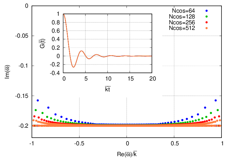
As we saw in the previous chapter the eigenvalues of the RTA should be two hydrodynamic poles and one cut located at $-i/\tau_{R}$. Additionally to the cut there are some aberrations at the edge of the cut that lean upwards in imaginary axis direction. To check if the deviations from the expected behavior are under control we analyze the effects of the discretization in the following. The increase of $N_{p}$ converges very quickly into a final solution with $N_{p}=64$ both in the time evolved Green’s function $G(t)$ and the eigenvalue picture in the complex frequency plane. Thus we will only discuss the influence of $N_{\cos\theta}$ by varying $N_{\cos\theta}$ and holding $N_{p}$ constant at $N_{p}=16$. The results are presented in Fig.3, where the eigenvalues for various discretizations are plotted in the complex frequency plane for $\bar{k}=1$. We can directly see that by increasing $N_{\cos\theta}$ we push the deviation of the eigenvalues at the edges of the cut down towards the cut, telling us that these deviations from the expected cut are purely discretization effects. We also have to look at the effects of $N_{\cos\theta}$ on the time dependent Green’s function $G(t)$. The results of this are found in the inset plot of Fig.3, where the same coloring as the eigenvalue plot is used to display different discretizations. For $N_{\cos\theta}=64$ the time evolution already reached its limit because further increase $N_{\cos\theta}$ does not change the function or at least only minimally for very late times. We conclude that discretization effects can be erased in the time evolved Green’s function entirely by using a feasible discretization. The eigenvalue picture however requires a high $N_{\cos\theta}$ to come close to the analytic cut expected in RTA, which is not numerically feasible under the consideration of also using $N_{p}=64$. The effects of the discretization are rather easy to discern from the physics here, thus we use a discretization of $N_{p}\times N_{\cos\theta}=64\times 64$ and keep in mind that the slight arcs of the cut are artificial.

Before we address the analytic structure of the Green’s functions at finite wave-number, the first result we should reproduce concerns the analytic structure of the Green’s function in the absence of gradients ($\bar{k}=0$). As already shown in Moore:2018mma the Green’s function for vanishing gradients exhibits a branch cut located on the imaginary axis.

In order to analyze this behavior, we investigate the spectrum of eigenvalues of the evolution operator, which in the absence of gradients only consists of the collision operator. Our results show three distinct zero modes which correspond to the conservation of energy, momentum and particle number in the sound channel. Other than that the spectrum only contains eigenvalues which are located on the imaginary frequency axis. In order to analyze whether this spectrum is discrete or continuous, one has to investigate how the eigenvalue density and their respective contribution to physical observables behaves in the continuum limit.
As objects to study these properties with we choose the eigenvalue density $\rho(\bar{\omega})$ and residue density $\rho_{\mu}(\bar{\omega})$. Since all eigenvalues have no real frequency $\text{Re}(\bar{\omega})$ the densities are calculated with respect to the imaginary frequency $\text{Im}(\bar{\omega})$. The eigenvalue density is calculated by counting all eigenvalues $\lambda_{i}$ in a frequency bin of size $\Delta\bar{\omega}$ with the help of the step function $\Theta_{j}(\bar{\omega}_{i},\bar{\omega})$ which is defined as

$\displaystyle\Theta_{j}(\bar{\omega}_{i},\bar{\omega})=\Theta\big(\Delta\bar{\omega}-2|\text{Im}(\bar{\omega})_{i}-(j+1/2)\Delta\bar{\omega}|\big)\Theta\big(\Delta\bar{\omega}-2|\text{Im}(\bar{\omega})-(j+1/2)\Delta\bar{\omega}|\big),$

(64)

where $\bar{\omega}_{i}$ is the frequency of each eigenvalue, as seen in Eq.(16). Normalizing this by the total number of eigenvalues, ignoring the three zero modes, we receive the eigenvalue density

$\displaystyle\rho(\bar{\omega})=\sum_{i=1}^{N_{tot}-3}\sum_{j=0}^{\infty}\frac{\Theta_{j}(\bar{\omega}_{i},\bar{\omega})}{(N_{tot}-3)\Delta\bar{\omega}}.$

(65)

In order to study a non-trivial residue density a suitable observable has to be chosen. All conserved charges have vanishing residue for $\bar{\omega}\neq 0$, hence a non conserved charge has to be used. As observable we consequently choose the momentum squared

$\displaystyle\vec{O}_{p^{2}}=\begin{pmatrix}p_{1_{p}}^{2}\\ p_{2_{p}}^{2}\\ \vdots\\ p_{Ntot_{p}}^{2}\end{pmatrix}.$

(66)

The residue $\mu_{i}$ of this observable per eigenvalue is given by Eq.(43). We have to sum this, analogously to the eigenvalue density, in a frequency bin $\Delta\bar{\omega}$ and normalize it. Here we don’t normalize by the total number of eigenvalues but the total residue of eigenvalues with $\bar{\omega}\neq 0$, which is subject to small variations due to the change in discretization²² 2 These variations are negligible and don’t change the physics but rather disturb the purpose of this analysis.. If we define this total non-conserved residue as

$\displaystyle\mu=\sum_{i=0}^{N_{tot}-3}\mu_{i},$

(67)

we can write the residue density of the non-conserved observable as

$\displaystyle\rho_{\mu}(\bar{\omega})=\sum_{i=1}^{N_{tot}-3}\sum_{j=0}^{\infty}\frac{\mu_{i}\Theta_{j}(\bar{\omega}_{i},\bar{\omega})}{\mu\Delta\bar{\omega}},$

(68)

where we also ignore the three zero modes in the sum. Since for our choice of initial condition (c.f Eq.(8)), the angular structure is trivial for $\bar{k}=0$, the discretization analysis is carried out by varying the number of momentum points $N_{p}$, which refines the discretization and the momentum cut-off $p_{max}$, which can be used to explore the addition of high momentum modes.
We illustrate the results in Fig.4 by plotting the eigenvalue density $\rho(\bar{\omega})$ in the bottom panel and the residue density $\rho_{\mu}(\omega)$ in the top panel. Each discretization is presented by a different color. The first thing to notice in the bottom panel is that the increase in $p_{max}$ corresponds to an addition of eigenvalues in the low frequency regime close to the origin, such that the number of eigenvalues decreases in higher frequency regions compared to discretizations with the same $N_{p}$. Vice versa when we fix $p_{max}$ and increase the number of momenta $N_{p}$ the density seems to approach a smooth continuum limit for each value of the momentum cut-off. Since the variation in $p_{max}$ induces strong changes in the eigenvalue density we have to check if this influences the physical properties of the system. For this see the top panel of Fig.4. Here we also see that additional low frequency eigenvalues get added when we increase $p_{max}$ but all of them have exponentially small residue, thus making them negligible for the linear response of the system. The increase in $N_{p}$ has the same influence on the residue density as on the eigenvalue density. By simultaneously increasing $p_{max}$ and $N_{p}$, the residue density seems to approach a genuine continuum limit with better and better discretization. We conclude that in the continuum limit $N_{p},p_{max}\rightarrow\infty$ the eigenvalues are continuously distributed along the negative imaginary frequency axis, representing a branch cut, which is in line with the prior works of Moore Moore:2018mma. While the branch cut terminates only at the real frequency axis, the contribution of points close to the real axis to physical observables is exponentially suppressed, as the dominant contribution originates from points with $\text{Im}(\bar{\omega})\sim 0.1$.

Now that we have established that the zero gradient spectrum is a branch cut we will discuss the effects of adding gradients to the Boltzmann equation. Before we discuss the results we should analyze how the discretization plays into it. We denote a certain discretization by $N_{p}\times N_{\cos\theta}$. For the results later in this work we choose a discretization of $64\times 64$ and $p_{max}/T=16$. In Fig.5 we present the results for three different discretizations for $\bar{k}=0.8$ in comparison with the final $64\times 64$ and $p_{max}/T=16$ discretization.

Eigenvalues of the evolution matrix are plotted in the top row and bottom left panel, with the hydrodynamic eigenvalues highlighted as big dots because they carry the largest individual residue for $\bar{k}=0.8$. By increasing the number of angles we see that we get a finer distribution of eigenvalues in the real range of frequencies, as seen in the top right panel. Equivalently we see a refinement in the imaginary frequencies by increasing the number of momenta, as seen in the bottom left panel. Although this yields more eigenvalues the overall picture of the complex plane stays the same, especially the positions of the hydrodynamic poles do not move. When we increase the maximum momentum cut-off, as in the top left panel, we see that we gather more eigenvalues closer to the real axis, as we have already seen for the case of $\bar{k}=0$. But again this does not change the position of hydrodynamic eigenvalues. Despite the various refinements in the complex frequency plane, the real time Green’s functions, plotted in the bottom right panel of Fig.5, shows the same behavior, where all curves of various discretizations lie on top of each other.
This discretization test shows that the discretization of $64\times 64$ with $p_{max}/T=16$ is well suited for the study of the complex structure of scalar theory. The further increase in discretization only added eigenvalues with small residues which did not change the complex structure at all and left the eigenvalues with the largest residues untouched. The physical description of observables, represented by the Green’s function, remains completely unchanged upon further refinement.

When one switches to non zero gradients the appearance of hydrodynamic modes is one of the first things happening for very small $\bar{k}$. The zero modes observed for $\bar{k}=0$, responsible for conservation laws, become hydrodynamic modes in the finite $\bar{k}$ case. All the other modes describe the non-hydrodynamic behavior.
Since in our calculation we only receive the location of eigenvalues $\lambda_{i}$ and their contribution $\mu_{i}$ to the Green’s function, we first need to come up with a definition for what we call hydrodynamic mode and how we isolate it in our data. We define the hydrodynamic modes, where possible (more on that later), as the complex conjugated pair of modes with the largest residue, which is obviously true for small $\bar{k}$. By identifying these modes for various $\bar{k}$, we can then obtain the dispersion relation $\bar{\omega}(\bar{k})$ of hydrodynamic sound modes, which is shown in Fig. 6 for both scalar theory and RTA as a comparison.

While at small $\bar{k}$, the dispersion relations for the real (left) and imaginary (right) part of the sound mode agree with second order viscous hydrodynamics, sizeable deviations start to occur for $\bar{k}\gtrsim 0.15$, and increase with increasing gradient strength, which is in line with the results reported in Du:2023bwi. Beyond $\bar{k}\approx 1.2$ the residue of the hydrodynamic mode extracted from scalar theory shrinks dramatically, as the mode disappears into a continuum of non-hydrodynamic excitations, and it is no longer meaningful to distinguish this mode from other excitations of the system, which is the reason that the curves in Fig. 6 terminate at this value of $\bar{k}$. Strikingly, a very similar behavior can also be seen in the Relaxation Time Approximation, where the hydrodynamic modes exhibit essentially the same dispersion relations up to $\bar{k}\sim 0.9$, where the hydrodynamic modes in RTA disappear behind the branch cut.
Now that we have established the behavior of the hydrodynamic sound mode, we continue to further analyze the behavior of the Green’s functions and in particular investigate the structure and impact of non-hydrodynamic excitations. In order to perform this analysis, we monitor the behavior of the Green’s functions in the real-time and real and complex frequency space, while varying the wave-number $\bar{k}$, which characterizes the magnitude of spatial gradients. Our results are compactly summarized in Figs. 7 and 8, where each row shows the behavior of the Green’s function for a fixed value of $\bar{k}$, with increasing $\bar{k}$ from top to bottom. In each row, the left most column shows the behavior of the real time Green’s functions $G(\bar{t})$ (see Eq.(42)), along with a decomposition into the contributions from the hydrodynamic sound mode (i.e. the complex conjugated pair of modes with the largest residue) and the non-hydrodynamic modes (i.e. all other), which can be reconstructed by summing only the contributions of the respective modes in Eq.(42). In the second column from the left, we depict the real and imaginary parts of the Green’s function $G(\bar{\omega})$ (see Eq.(44)) as a function of real frequencies $\bar{\omega}/\bar{k}$. The behavior in the complex frequency plane is elucidated in the third column of Figs. 7 and 8, where black circles show the location of individual eigenvalues calculated from the matrix, which are scaled in size by their contribution $\mu_{i}$ to the Green’s function, while the color code in these plots corresponds to the logarithm of the absolute square of the Green’s function.³³ 3 Note that one does not see every eigenvalue here because some have such a small contribution that their sizes are scaled to be invisible, so one only sees eigenvalues that have at least some influence on the Green’s function. Finally, the right most plot is a histogram showing the summed contributions $\rho_{\mu}(\bar{\omega})$ from non-hydrodynamic modes as defined in Eq.(68). Since there can be both positive and negative contributions, we distinguish them by a color coding, where positive contributions are plotted in red and negative contributions in blue. Contributions of the non-hydrodynamic modes are further compared to the contribution of the the hydrodynamic sound mode, which is indicated by a green bar.
When considering the behavior of the real-time Green’s function $G(t)$ (left column), we find that for small gradients $\bar{k}\ll 1$ the evolution is almost purely hydrodynamic, meaning that only the complex conjugated pair of modes with the largest residue play a significant role for the time evolution of the system. With increasing $\bar{k}$, the contribution of non-hydrodynamic modes becomes visible at early times, but exhibits a much faster decay than the hydrodynamic contribution. When $\bar{k}\sim 1$, the contributions from hydrodynamic and non-hydrodynamic modes become of comparable size, until for $\bar{k}\approx 1.2$ the contribution of the hydrodynamic mode begins to disappear as non-hydrodynamic modes start to dominate the behavior of the real-time Green’s function. By $\bar{k}=1.5$, corresponding to the largest value shown in Fig.8, it is then no longer possible to identify a clear signature of a hydrodynamic mode in the system.

Next we consider the Green’s function $G(\bar{w})$ as a function of real frequency $\bar{\omega}$ (second left column), which for small gradients $(\bar{k}\ll 1)$ features two distinct peaks in its real part and at the same position two steep inflection points in the imaginary part. Clearly, these features are a sign of the contribution of two very distinct regions in the complex frequency plane, in this case the hydrodynamic poles, which for $\bar{k}\ll 1$ are located close to real frequency axis. By increasing $\bar{k}$ the influence of the hydrodynamic poles diminishes, as their residues shrink and they move away from the real-frequency axis, leading to a broadening of peaks and inflections. Nevertheless, both the real-time and the real-frequency Green’s functions exhibit a remarkably smooth behavior with increasing $\bar{k}$, and do not immediately indicate a transition from a hydrodynamic to a non-hydrodynamic regime.

Now, if we consider the behavior of the Green’s function in the complex frequency plane (right two columns), for small $\bar{k}\ll 1$ we can clearly see the dominance of the hydrodynamic modes, which correspond to simple poles in the complex frequency plane with large residues. However, in addition to the hydrodynamic poles, additional singularities indicated by black circles appear throughout the region where $-\bar{k}<\text{Re}(\bar{\omega})<\bar{k}$ and $\text{Im}(\bar{\omega})<0$, which most likely signals the presence of an entire region of non-analyticity as discussed in Kurkela:2017xis for the momentum dependent relaxation time approximation. Despite the fact that the singularities cover a large region in the complex frequency plane, it appears that the dominant contribution to the Green’s function of the energy-momentum tensor seems to be located around $\text{Im}(\bar{\omega})\approx-0.2$, as can be seen from the residue density in the right most panel, which reminiscent of the $\bar{k}=0$ spectrum in Fig. 4 is also strongly peaked around a single imaginary part of the frequency. Hence, the typical time scale for the relaxation of contributions of non-hydrodynamic modes to the energy-momentum tensor is still given by the inverse of this characteristic frequency $\sim 1/\text{Im}(\bar{\omega})\approx 5$, which is in line with the value of the second order transport coefficient $\bar{\tau}_{\pi}\approx 6.1$ York:2008rr. Due to this rather strong peak in the residue density, the behavior of the Green’s function in scalar $\phi^{4}$ theory is actually not to different from the behavior in the conformal relaxation time approximation (see also  Du:2023bwi) where – instead of a spread out region in the complex frequency plane – the non-hydrodynamic contributions originates from a single branch-cut located at $\text{Im}(\bar{\omega})=-1/\bar{\tau}_{R}=0.2$.

References

- (1) ALICE collaboration, Multiparticle azimuthal correlations in p -Pb and Pb-Pb collisions at the CERN Large Hadron Collider, Phys. Rev. C 90 (2014) 054901 [1406.2474].
- (2) ATLAS collaboration, Measurement of multi-particle azimuthal correlations in , Pb and low-multiplicity PbPb collisions with the ATLAS detector, Eur. Phys. J. C 77 (2017) 428 [1705.04176].
- (3) CMS collaboration, Observation of Correlated Azimuthal Anisotropy Fourier Harmonics in and Collisions at the LHC, Phys. Rev. Lett. 120 (2018) 092301 [1709.09189].
- (4) J.L. Nagle and W.A. Zajc, Small System Collectivity in Relativistic Hadronic and Nuclear Collisions, Ann. Rev. Nucl. Part. Sci. 68 (2018) 211 [1801.03477].
- (5) R. Baier, P. Romatschke and U.A. Wiedemann, Dissipative hydrodynamics and heavy ion collisions, Phys. Rev. C 73 (2006) 064903 [hep-ph/0602249].
- (6) D.A. Teaney, Viscous Hydrodynamics and the Quark Gluon Plasma, in Quark-gluon plasma 4, R.C. Hwa and X.-N. Wang, eds., pp. 207–266 (2010), DOI [0905.2433].
- (7) H. Song, S.A. Bass, U. Heinz, T. Hirano and C. Shen, 200 A GeV Au+Au collisions serve a nearly perfect quark-gluon liquid, Phys. Rev. Lett. 106 (2011) 192301 [1011.2783].
- (8) R. Snellings, Elliptic Flow: A Brief Review, New J. Phys. 13 (2011) 055008 [1102.3010].
- (9) B. Schenke, S. Jeon and C. Gale, Elliptic and triangular flows in 3 + 1D viscous hydrodynamics with fluctuating initial conditions, J. Phys. G 38 (2011) 124169.
- (10) U. Heinz and R. Snellings, Collective flow and viscosity in relativistic heavy-ion collisions, Ann. Rev. Nucl. Part. Sci. 63 (2013) 123 [1301.2826].
- (11) M. Luzum and H. Petersen, Initial State Fluctuations and Final State Correlations in Relativistic Heavy-Ion Collisions, J. Phys. G 41 (2014) 063102 [1312.5503].
- (12) C. Gale, S. Jeon and B. Schenke, Hydrodynamic Modeling of Heavy-Ion Collisions, Int. J. Mod. Phys. A 28 (2013) 1340011 [1301.5893].
- (13) J. Berges, K. Boguslavski, S. Schlichting and R. Venugopalan, Universal attractor in a highly occupied non-Abelian plasma, Phys. Rev. D 89 (2014) 114007 [1311.3005].
- (14) P. Bozek, Collective flow in p-Pb and d-Pd collisions at TeV energies, Phys. Rev. C 85 (2012) 014911 [1112.0915].
- (15) V.E. Ambrus, S. Schlichting and C. Werthmann, Development of transverse flow at small and large opacities in conformal kinetic theory, Phys. Rev. D 105 (2022) 014031 [2109.03290].
- (16) V.E. Ambrus, S. Schlichting and C. Werthmann, Establishing the Range of Applicability of Hydrodynamics in High-Energy Collisions, Phys. Rev. Lett. 130 (2023) 152301 [2211.14356].
- (17) B. Schenke, S. Schlichting and P. Singh, Tracing the Emergence of Collectivity Phenomena in Small Systems, Acta Phys. Polon. Supp. 16 (2023) 79 [2212.02278].
- (18) G.S. Denicol, T. Koide and D.H. Rischke, Dissipative relativistic fluid dynamics: a new way to derive the equations of motion from kinetic theory, Phys. Rev. Lett. 105 (2010) 162501 [1004.5013].
- (19) P. Kovtun, Lectures on hydrodynamic fluctuations in relativistic theories, J. Phys. A 45 (2012) 473001 [1205.5040].
- (20) P. Romatschke and U. Romatschke, Relativistic Fluid Dynamics In and Out of Equilibrium, Cambridge Monographs on Mathematical Physics, Cambridge University Press (5, 2019), 10.1017/9781108651998, [1712.05815].
- (21) J. Casalderrey-Solana, N.I. Gushterov and B. Meiring, Resurgence and Hydrodynamic Attractors in Gauss-Bonnet Holography, JHEP 04 (2018) 042 [1712.02772].
- (22) J.-P. Blaizot and L. Yan, Emergence of hydrodynamical behavior in expanding ultra-relativistic plasmas, Annals Phys. 412 (2020) 167993 [1904.08677].
- (23) J. Casalderrey-Solana, H. Liu, D. Mateos, K. Rajagopal and U.A. Wiedemann, Gauge/String Duality, Hot QCD and Heavy Ion Collisions, Cambridge University Press (2014), 10.1017/CBO9781139136747, [1101.0618].
- (24) M.P. Heller, D. Mateos, W. van der Schee and M. Triana, Holographic isotropization linearized, JHEP 09 (2013) 026 [1304.5172].
- (25) G.S. Denicol, U.W. Heinz, M. Martinez, J. Noronha and M. Strickland, New Exact Solution of the Relativistic Boltzmann Equation and its Hydrodynamic Limit, Phys. Rev. Lett. 113 (2014) 202301 [1408.5646].
- (26) M.P. Heller and M. Spalinski, Hydrodynamics Beyond the Gradient Expansion: Resurgence and Resummation, Phys. Rev. Lett. 115 (2015) 072501 [1503.07514].
- (27) A. Kurkela and Y. Zhu, Isotropization and hydrodynamization in weakly coupled heavy-ion collisions, Phys. Rev. Lett. 115 (2015) 182301 [1506.06647].
- (28) P. Romatschke, Do nuclear collisions create a locally equilibrated quark–gluon plasma?, Eur. Phys. J. C 77 (2017) 21 [1609.02820].
- (29) P. Romatschke, Relativistic Fluid Dynamics Far From Local Equilibrium, Phys. Rev. Lett. 120 (2018) 012301 [1704.08699].
- (30) J. Berges, M.P. Heller, A. Mazeliauskas and R. Venugopalan, QCD thermalization: Ab initio approaches and interdisciplinary connections, Rev. Mod. Phys. 93 (2021) 035003 [2005.12299].
- (31) P. Romatschke, Retarded correlators in kinetic theory: branch cuts, poles and hydrodynamic onset transitions, Eur. Phys. J. C 76 (2016) 352 [1512.02641].
- (32) S. Grozdanov and A.O. Starinets, Second-order transport, quasinormal modes and zero-viscosity limit in the Gauss-Bonnet holographic fluid, JHEP 03 (2017) 166 [1611.07053].
- (33) A. Kurkela and U.A. Wiedemann, Analytic structure of nonhydrodynamic modes in kinetic theory, Eur. Phys. J. C 79 (2019) 776 [1712.04376].
- (34) G.D. Moore, Stress-stress correlator in theory: poles or a cut?, JHEP 05 (2018) 084 [1803.00736].
- (35) A. Soloviev, Hydrodynamic attractors in heavy ion collisions: a review, Eur. Phys. J. C 82 (2022) 319 [2109.15081].
- (36) J. Brewer, W. Ke, L. Yan and Y. Yin, Far-from-equilibrium slow modes and momentum anisotropy in expanding plasma, 2212.00820.
- (37) W. Ke and Y. Yin, Does a Quark-Gluon Plasma Feature an Extended Hydrodynamic Regime?, Phys. Rev. Lett. 130 (2023) 212303 [2208.01046].
- (38) X. Du, S. Ochsenfeld and S. Schlichting, Universality of energy-momentum response in kinetic theories, 2306.09094.
- (39) I. Muller, Zum Paradoxon der Warmeleitungstheorie, Z. Phys. 198 (1967) 329.
- (40) W. Israel and J.M. Stewart, Transient relativistic thermodynamics and kinetic theory, Annals Phys. 118 (1979) 341.
- (41) R. Baier, P. Romatschke, D.T. Son, A.O. Starinets and M.A. Stephanov, Relativistic viscous hydrodynamics, conformal invariance, and holography, JHEP 04 (2008) 100 [0712.2451].
- (42) P. Romatschke, New Developments in Relativistic Viscous Hydrodynamics, Int. J. Mod. Phys. E 19 (2010) 1 [0902.3663].
- (43) G.S. Denicol, H. Niemi, E. Molnar and D.H. Rischke, Derivation of transient relativistic fluid dynamics from the Boltzmann equation, Phys. Rev. D 85 (2012) 114047 [1202.4551].
- (44) P.B. Arnold, G.D. Moore and L.G. Yaffe, Effective kinetic theory for high temperature gauge theories, JHEP 01 (2003) 030 [hep-ph/0209353].
- (45) A. Kurkela and E. Lu, Approach to Equilibrium in Weakly Coupled Non-Abelian Plasmas, Phys. Rev. Lett. 113 (2014) 182301 [1405.6318].
- (46) J.-P. Blaizot, B. Wu and L. Yan, Quark production, Bose–Einstein condensates and thermalization of the quark–gluon plasma, Nucl. Phys. A 930 (2014) 139 [1402.5049].
- (47) Z. Xu, K. Zhou, P. Zhuang and C. Greiner, Thermalization of gluons with Bose-Einstein condensation, Phys. Rev. Lett. 114 (2015) 182301 [1410.5616].
- (48) F. Scardina, D. Perricone, S. Plumari, M. Ruggieri and V. Greco, Relativistic Boltzmann transport approach with Bose-Einstein statistics and the onset of gluon condensation, Phys. Rev. C 90 (2014) 054904 [1408.1313].
- (49) A. Kurkela, A. Mazeliauskas, J.-F. Paquet, S. Schlichting and D. Teaney, Matching the Nonequilibrium Initial Stage of Heavy Ion Collisions to Hydrodynamics with QCD Kinetic Theory, Phys. Rev. Lett. 122 (2019) 122302 [1805.01604].
- (50) A. Kurkela and A. Mazeliauskas, Chemical equilibration in weakly coupled QCD, Phys. Rev. D 99 (2019) 054018 [1811.03068].
- (51) P. Carzon, M. Martinez, J. Noronha-Hostler, P. Plaschke, S. Schlichting and M. Sievert, Pre-Equilibrium Evolution of Conserved Charges with ICCING Initial Conditions, 2301.04572.
- (52) A. Muronga, Relativistic Dynamics of Non-ideal Fluids: Viscous and heat-conducting fluids. II. Transport properties and microscopic description of relativistic nuclear matter, Phys. Rev. C 76 (2007) 014910 [nucl-th/0611091].
- (53) B. Betz, D. Henkel and D.H. Rischke, Complete second-order dissipative fluid dynamics, J. Phys. G 36 (2009) 064029.
- (54) G.D. Moore, Next-to-Leading Order Shear Viscosity in lambda phi**4 Theory, Phys. Rev. D 76 (2007) 107702 [0706.3692].
- (55) M.A. York and G.D. Moore, Second order hydrodynamic coefficients from kinetic theory, Phys. Rev. D 79 (2009) 054011 [0811.0729].
- (56) M.C. Abraao York, A. Kurkela, E. Lu and G.D. Moore, UV cascade in classical Yang-Mills theory via kinetic theory, Phys. Rev. D 89 (2014) 074036 [1401.3751].
- (57) X. Du and S. Schlichting, Equilibration of weakly coupled QCD plasmas, Phys. Rev. D 104 (2021) 054011 [2012.09079].
- (58) N. Mullins, G.S. Denicol and J. Noronha, Far-from-equilibrium kinetic dynamics of 4 theory in an expanding universe, Phys. Rev. D 106 (2022) 056024 [2207.07786].
- (59) I. Soudi, Energy loss and equilibration of a highly energetic parton in QCD plasmas, Ph.D. thesis, Bielefeld U., 2021. 10.4119/unibi/2958574.
- (60) G.S. Rocha, M.N. Ferreira, G.S. Denicol and J. Noronha, Transport coefficients of quasiparticle models within a new relaxation time approximation of the Boltzmann equation, Phys. Rev. D 106 (2022) 036022 [2203.15571].
- (61) S. Jeon and L.G. Yaffe, From quantum field theory to hydrodynamics: Transport coefficients and effective kinetic theory, Phys. Rev. D 53 (1996) 5799 [hep-ph/9512263].
- (62) J. Berges and S. Borsanyi, Range of validity of transport equations, Phys. Rev. D 74 (2006) 045022 [hep-ph/0512155].
- (63) S. Weinstock, Boltzmann collision term, Phys. Rev. D 73 (2006) 025005 [hep-ph/0510417].
- (64) J. Berges, Introduction to nonequilibrium quantum field theory, AIP Conf. Proc. 739 (2004) 3 [hep-ph/0409233].