Converting long-range entanglement into mixture: tensor-network approach to local equilibration
Abstract
In the out-of-equilibrium evolution induced by a quench, fast degrees of freedom generate long-range entanglement that is hard to encode with standard tensor networks. However, local observables only sense such long-range correlations through their contribution to the reduced local state as a mixture. We present a tensor network method that identifies such long-range entanglement and efficiently transforms it into mixture, much easier to represent. In this way, we obtain an effective description of the time-evolved state as a density matrix that captures the long-time behavior of local operators with finite computational resources.

Reconciling the time-reversal invariant unitary evolution of closed quantum many-body systems with the emergence of statistical mechanics and its well defined arrow of time is still an open question, hindered by the exponential complexity of simulating this problem in the generic case.
In contrast to the dynamical scenario, the equilibrium wave functions of a large class of physically relevant systems live in a small corner of the exponentially large Hilbert space. Such corner is characterized by a bounded amount of entanglement Eisert et al. 2010 and states therein admit an efficient approximation as a tensor network (TN) Cirac et al. 2021. This property implies we can perform very precise numerical simulations with only polynomial resources Verstraete et al. 2008; Schollwöck 2011; Orús 2014; Silvi et al. 2019; Ran et al. 2020; Okunishi et al. 2021; Bañuls 2023. The most notable example of successful TN simulations are those in one-dimension performed with matrix product states (MPS) Fannes et al. 1992; White 1992; Östlund and Rommer 1995; Pérez-García et al. 2007; Schollwöck 2011.
Out of equilibrium, instead, initially localized correlations can propagate over arbitrarily large distances. As a result, the entanglement in the system increases rapidly with time Calabrese and Cardy 2005; Osborne 2006; Schuch et al. 2008; Läuchli and Kollath 2008; Rossini et al. 2010; Van Acoleyen et al. 2013 and simple TN ansatzes such as MPS have limited applicability. The exponential complexity of the full quantum state evolution originates from an extremely non-local pattern of correlations, and might be circumvented by focusing instead on a local description of the state. Significant simplifications using this approach have already been observed Bañuls et al. 2009; Leviatan et al. 2017; White et al. 2018; Hallam et al. 2019; Krumnow et al. 2019; Pastori et al. 2019; Surace et al. 2019; Rams and Zwolak 2020; Rakovszky et al. 2022; Kvorning et al. 2022; Frías-Pérez and Bañuls 2022.
Here we develop this idea and propose a new algorithm that explicitly identifies long-range entanglement in the system and trades it for mixture (see also Surace et al. 2019). In particular, our method focuses on separating fast and slow propagating degrees of freedom. Already from an early time we here observe that the fast degrees of freedom mediate non-local correlations whose effect on local observables is similar to that of a statistical mixture.
By trading such correlations for the corresponding mixture we devise a TN algorithm that allows to simulate the evolution of local observables for considerably longer times than what was achievable before, with finite computational resources. In fact, our algorithm provides an effective description of the time-evolved state as a density matrix, represented by a matrix product operator (MPO) with bounded bond dimension, that accurately captures the long-time behavior of local operators.
We support these claims by providing benchmark numerical results for quenches in the transverse field Ising model and its non-integrable generalization. We find that our algorithm predicts accurately the long-time values of local observables as dictated by, respectively, the analytical solutions and the prediction of the diagonal ensemble Srednicki 1994; Gogolin and Eisert 2016; Vidmar and Rigol 2016.


Quenches and quasiparticles.
We focus on the out-of-equilibrium dynamics induced by quantum quenches Calabrese and Cardy 2005; Mitra 2018, in which a one-dimensional system in the thermodynamic limit is prepared at in a product state , and later evolved with an entangling Hamiltonian . Our aim is to compute the time-dependent expectation value of a local observable .
The initial state has a finite energy density above the ground state, and thus a large occupation of excited states, often described as quasiparticles states (QP). The subsequent dynamics can be described as the radiation of entangled pairs of QPs Calabrese and Cardy 2005. In translational invariant systems indeed QPs possess a well-defined energy-momentum dispersion relation , and a QP wave-packet centered at propagates with group velocity , while momentum conservation enforces equal occupation of and states that propagate in opposite directions.
Identifying long-distance entanglement.
In order to identify the long-distance contributions to the entanglement we need to focus on a subsystem of neighboring spins, and label and the remaining left and right regions of the system (see Fig. 1). Entanglement across a bipartition (e.g. vs ) is created by correlated pairs of QPs with support on both sides of the cut. We define as long-distance entanglement the contribution to the entanglement generated by any QP pair supported on and , but not on .
We can visualize this in the cartoon of Fig. 1(a), where we consider a quench that excites a single pair of entangled QPs, initially located inside , that later travel with opposite velocities . 11 1 This kind of simple dynamics is actually realized in a toy model of local unitaries Bañuls et al. 2009; Müller-Hermes et al. 2012 and in some concrete physical realizations such as the split quenches studied in Zamora et al. 2014; Chen and Vidal 2014. . In this simple example, becomes entangled with the rest when one member of the pair leaves the region, but when both QPs have left, after , is again in a product state with respect to . At this stage we can factorize the total state into the product of an entangled state of and a state of .
In a more general scenario such complete factorization is not possible, since and might contain other sources of entanglement. The simplest generalization depicted in Fig. 1(b) involves two pairs of QPs, one fast (orange) and one slow (blue). When the former has left the latter is still partially in . At that stage, it is still possible to disentangle a part of and from . We can indeed identify a factorization of the Hilbert spaces, and , such that the subsystem is not entangled with . In the simple scenario presented above, is defined by the degrees of freedom that describe the fast pair, and we can factorize the state as , where the second factor captures the pair of fast modes.
Trading long-distance entanglement for mixture.
In a translationally invariant system, we can repeat the cartoon picture above for each block of sites. When computing the expectation value of a local observable, we need to trace out all the degrees of freedom but the ones where the observable is defined. Given that fast constituents of entangled pairs of QP are separated by at least sites, one of the two partners will always be traced out in this procedure leaving the other in a mixed state.
Thus, when focusing on local observables, we can describe the system as a mixed state, originated by having discarded the coherence between each pair of fast QP. Their joint pure entangled state is substituted by a mixed state built as the product of the two mixed states obtained by tracing out the partner in the pair,
| (1) |
where are the reduced density matrices of each QP. This provides a more efficient local description in terms of entanglement, as the long-distance components have been removed.
From the QP intuition to a TN algorithm.
We can use the above observation in an actual TN algorithm. Standard MPS algorithms for this setup attempt to represent the time-evolved state as a MPS, parametrized by one or few tensors of small size , where is the physical dimension of the chain sites and the bond dimension Vidal 2007a; Haegeman et al. 2011; Vanderstraeten et al. 2019a. Since the half-chain entropy of the MPS is upper-bounded by Perez-Garcia et al. 2007; Schollwöck 2011; Evenbly and Vidal 2011, the typical linear growth in time of entropy after a quench Calabrese and Cardy 2005; Schuch et al. 2008 requires an exponential increase of the tensors dimensions to maintains a constant precision. As a result, given finite computational resources, standard TN algorithms Paeckel et al. 2019 only give reliable predictions for relatively short times (typically of the order with the relevant energy scale).
Translating the QP intuition above to the TN setting we can however obtain a more efficient TN description for the local observables. Let us, for simplicity, assume that each MPS tensor represents precisely sites 22 2 This can be always obtained by blocking together tensors of the original systems to yield a single tensor.. Singling out one subsystem, the whole state can thus be written as
| (2) |
where the sum is over orthonormal bases of the block and its left and right environments , meaning that we use the gauge in which the tensor for the subsystem is the orthogonality center of the MPS Vidal 2007a; Pérez-García et al. 2007; Vanderstraeten et al. 2019b; Evenbly 2022.
If there are long-range entangled degrees of freedom that decouple from , the state will have a product structure, with one component completely disentangled from the physical degrees of freedom. There will thus exist basis transformations (disentanglers Vidal 2007b; Evenbly and Vidal 2009) on and identifying the decomposition and , such that
| (3) |
as depicted in Fig. 2(I.a). Assuming such and exist, they need to be determined variationally, for example by minimizing the Euclidean distance between the left and right-hand side of (3). Namely, given the evolved state in the form (2), and for fixed dimension of the long-range component, we iteratively optimize each of the disentanglers and and the vectors and until we reach the minimal possible Euclidean distance among the right and left hand sides of Eq. (3) Kraft et al. 2018. Since the dimension of the fast factors and is not known, the procedure needs to be repeated for different trial values.
Assuming the above procedure is successful, we now can transform the identified long-range entanglement into mixture by applying the substitution (1) to each consecutive subsystem in the chain. As schematically shown in Fig. 2(I.b), this exchanges the pure MPS description of the system by a mixed (purified) MPO with smaller bond dimension , at the expense of additional (purification) indices.
When the decomposition (3) is exact, this mixed state has the property that the reduced density matrices for (resp. ) are unchanged SM. As a consequence, also the reduced density matrix for two adjacent blocks, and thus all observables with support on up to sites are preserved. We can then continue the evolution with the original Hamiltonian acting on the physical indices. Fast degrees of freedom will continue propagating entanglement through the subsystem . Thus, the step of finding and mixing the long-range entangled components is repeated periodically.
An improved TN algorithm.
In practice, the optimal decomposition we are able to identify using the strategy just outlined still retains some residual entropy between fast and slow degrees of freedom . We apply the truncation when this entropy falls below a given threshold . This results into small errors when building the mixed state that reflect in the evolution of local observables [see Fig. 4(a)]. Therefore we introduce an improved heuristic TN algorithm, in which, after solving (3), if the residual entropy falls below we directly propose an effective purification ansatz, described by three rank-3 tensors with fixed dimensions , and , where is a chosen dimension for the purification index and [see Fig. 2(c)].
The purification tensors are found variationally by minimizing the distance between the reduced density matrices (and ) obtained from the original state (2) and from the purification. As initial guess we use the tensors obtained from solving (3), and we use gradient descent for the minimization problem (see SM) .
Notice that the number of purification legs increases after each mixing step. To handle this in practice, we group together all the purification indices between two physical sites and apply a cutoff to the total purification dimension 33 3 We apply the simplest cutoff, which uses a SVD of the purification vs. the virtual legs. Notice that other schemes would be possible to try and optimize the purification sites, for instance, in the spirit of the optimal purification of Hauschild et al. 2018. .
Numerical results.
We benchmark the algorithm using the transverse field Ising model with an additional integrability-breaking next-to-nearest neighbor interaction,
| (4) |
Initially in a product state , corresponding to the ground state deep in the paramagnetic phase (), the system is quenched to a finite value of the transverse field (and potentially ).
To explore systematically the structure of the time-evolved MPS, we simulate accurately the short-time evolution using the infinite time-evolving block decimation (iTEBD) algorithm Vidal 2007a with a large enough bond dimension. We then probe the disentangling of fast and slow degrees of freedom at different times solving (3) for a subsystem of sites for several quenches.
As shown in Fig. 3, after a certain time we can identify subsystems of and that practically disentangle from the local region and carry long-range entanglement between the environments, measured by the logarithmic negativity Vidal and Werner 2002 of the reduced density matrix for the fast degrees of freedom . For all quenches, the residual entanglement entropy between the fast degrees of freedom and the rest decays fast with time, at a slower rate when the quench is into the ordered phase 44 4 This is consistent with the distribution of momentum excitations in the initial state, computed in the exact free-fermionic formulation, which is peaked at finite velocities when the quench is within the same phase, and at zero velocity otherwise (see the supplementary material SM).. Also as expected, the time at which fast degrees of freedom start decoupling from the local system depends linearly on its size , as illustrated in the inset of Fig. 3(a)].
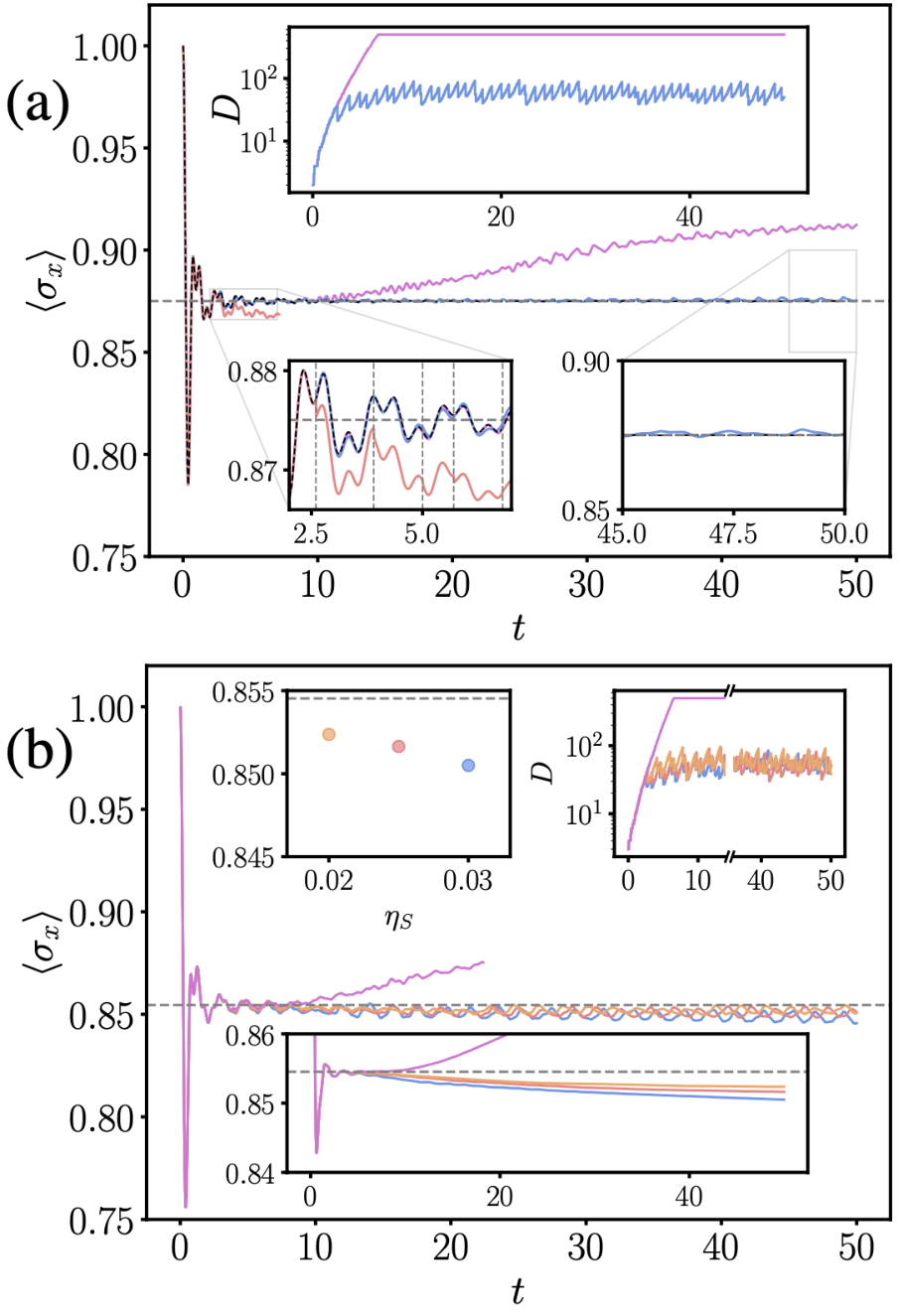
We now use the TN algorithm described above and check its performance simulating the long-time evolution of local observables. Fig. 4(b) shows the results for the integrable quench , and the only non-vanishing (due to the symmetry) single-site observable . Solving (3) and trading entanglement by mixture captures the qualitatively correct dynamics, but introduces discontinuous jumps (orange line and lower-left inset) that we attribute to the decomposition not being exact. The improved heuristic algorithm achieves much better results (blue line and lower-right inset). While the approximation induces some residual oscillations, these are very small and close to the exact equilibration results even after considerably long times. In contrast, the iTEBD results with a maximal bond dimension (pink line) start to severely deviate from the exact solution at around .
Our algorithm uses instead a much smaller bond dimension: during the time evolution steps, the required bond dimension of the purified MPS grows exponentially, but each time we trade some of the entanglement for mixture, the bond dimension gets halved 55 5 We use for our ansatz. As we iterate the procedure, the maximum required bond dimension tends to a constant (upper inset).
In Fig. 4(b) we repeat a similar analysis for the non-integrable quench , . The different colors show the results for different thresholds for the residual entropy . Smaller values require longer evolution between mixing steps, and thus larger bond dimension, but improve the results systematically.
Our results systematically approach the long-time limit predicted by the diagonal ensemble 66 6 Extrapolated from exact finite size results.. Even for the largest threshold, the relative error in the time-averaged value after is below (). Also the time-averaged magnetization exhibits a similar precision, as shown in the lower inset. Also in this case the largest bond dimension saturates with (upper right inset).
In the supplementary material, we also repeat the calculations in the integrable case directly using the free-fermionic formalism where we can track the coherence we discard in our simulation and confirm it does not play a relevant role in the long-time dynamics of local observables SM.
Discussion.
By identifying the long-range entanglement produced in the out-of-equilibrium dynamics after a quantum quench and converting it into mixture, we have proposed an explicit approach to avoid the entanglement barrier and simulate the out-of-equilibrium dynamics of an infinite quantum chain with MPS using finite computational resources.
Our approach is inspired by the intuitive understanding of entanglement dynamics in terms of the radiation of QP. It relies on the hypothesis that fast degrees of freedom propagate correlations to steadily growing distances, contributing to the linear growth of entanglement across the system, but only as statistical mixture to sufficiently local observables. Our numerical results for the Ising chain show that the intuition is accurate in the free-fermionic case, which best fits the QP picture.
We have generalized our intuition to a heuristic algorithm that goes beyond the QP picture and also performs well in non-integrable regimes of the model. It is thus important to pursue further characterization of the algorithm in order to chart its potential and limitations.
Acknowledgements.
LT would like to thank Jacopo Surace who has contributed to developing the original ideas that have motivated this work. This work was partially supported by the Deutsche Forschungsgemeinschaft (DFG, German Research Foundation) under Germany’s Excellence Strategy – EXC-2111 – 390814868; 499180199 and and by the EU-QUANTERA project TNiSQ (BA 6059/1-1). LT acknowledges support from the Proyecto Sinérgico CAM 2020 Y2020/TCS-6545 (NanoQuCo-CM), the CSIC Research Platform on Quantum Technologies PTI-001 and from Spanish projects PID2021-127968NB-I00 and TED2021-130552B-C22 funded by MCIN/AEI/10.13039/501100011033/FEDER, UE and MCIN/AEI/10.13039/501100011033, respectively.References
- Eisert et al. (2010) J. Eisert, M. Cramer, and M. B. Plenio, Rev. Mod. Phys. 82, 277 (2010).
- Cirac et al. (2021) J. I. Cirac, D. Pérez-García, N. Schuch, and F. Verstraete, Rev. Mod. Phys. 93, 045003 (2021).
- Verstraete et al. (2008) F. Verstraete, V. Murg, and J. Cirac, Adv. Phys. 57, 143 (2008).
- Schollwöck (2011) U. Schollwöck, Ann. Phys. 326, 96 (2011), january 2011 Special Issue.
- Orús (2014) R. Orús, Annals Phys. 349, 117 (2014).
- Silvi et al. (2019) P. Silvi, F. Tschirsich, M. Gerster, J. Jünemann, D. Jaschke, M. Rizzi, and S. Montangero, SciPost Phys. Lect. Notes , 8 (2019).
- Ran et al. (2020) S.-J. Ran, E. Tirrito, C. Peng, X. Chen, L. Tagliacozzo, G. Su, and M. Lewenstein, Tensor Network Contractions, Lecture Notes in Physics (Springer International Publishing, 2020).
- Okunishi et al. (2021) K. Okunishi, T. Nishino, and H. Ueda, (2021), arXiv:2111.12223 [cond-mat.stat-mech] .
- Bañuls (2023) M. C. Bañuls, Annual Review of Condensed Matter Physics 14, null (2023), https://doi.org/10.1146/annurev-conmatphys-040721-022705 .
- Fannes et al. (1992) M. Fannes, B. Nachtergaele, and R. F. Werner, Commun. Math. Phys. 144, 443 (1992).
- White (1992) S. R. White, Phys. Rev. Lett. 69, 2863 (1992).
- Östlund and Rommer (1995) S. Östlund and S. Rommer, Phys. Rev. Lett. 75, 3537 (1995).
- Pérez-García et al. (2007) D. Pérez-García, F. Verstraete, M. M. Wolf, and J. I. Cirac, Quantum Inf. Comput. 7, 401 (2007).
- Calabrese and Cardy (2005) P. Calabrese and J. Cardy, Journal of Statistical Mechanics: Theory and Experiment 2005, P04010 (2005).
- Osborne (2006) T. J. Osborne, Phys. Rev. Lett. 97, 157202 (2006).
- Schuch et al. (2008) N. Schuch, M. M. Wolf, K. G. H. Vollbrecht, and J. I. Cirac, New Journal of Physics 10, 033032 (2008).
- Läuchli and Kollath (2008) A. M. Läuchli and C. Kollath, Journal of Statistical Mechanics: Theory and Experiment 2008, P05018 (2008).
- Rossini et al. (2010) D. Rossini, S. Suzuki, G. Mussardo, G. E. Santoro, and A. Silva, Physical Review B 82, 144302 (2010).
- Van Acoleyen et al. (2013) K. Van Acoleyen, M. Mariën, and F. Verstraete, Phys. Rev. Lett. 111, 170501 (2013).
- Bañuls et al. (2009) M. C. Bañuls, M. B. Hastings, F. Verstraete, and J. I. Cirac, Phys. Rev. Lett. 102, 240603 (2009).
- Leviatan et al. (2017) E. Leviatan, F. Pollmann, J. H. Bardarson, D. A. Huse, and E. Altman, “Quantum thermalization dynamics with matrix-product states,” (2017), arXiv:1702.08894 [cond-mat.stat-mech] .
- White et al. (2018) C. D. White, M. Zaletel, R. S. K. Mong, and G. Refael, Phys. Rev. B 97, 035127 (2018).
- Hallam et al. (2019) A. Hallam, J. G. Morley, and A. G. Green, Nature Communications 10, 2708 (2019).
- Krumnow et al. (2019) C. Krumnow, J. Eisert, and Ö. Legeza, “Towards overcoming the entanglement barrier when simulating long-time evolution,” (2019), arXiv:1904.11999 [cond-mat.stat-mech] .
- Pastori et al. (2019) L. Pastori, M. Heyl, and J. C. Budich, Phys. Rev. Research 1, 012007 (2019).
- Surace et al. (2019) J. Surace, M. Piani, and L. Tagliacozzo, Phys. Rev. B 99, 235115 (2019).
- Rams and Zwolak (2020) M. M. Rams and M. Zwolak, Phys. Rev. Lett. 124, 137701 (2020).
- Rakovszky et al. (2022) T. Rakovszky, C. W. von Keyserlingk, and F. Pollmann, Phys. Rev. B 105, 075131 (2022).
- Kvorning et al. (2022) T. K. Kvorning, L. Herviou, and J. H. Bardarson, SciPost Phys. 13, 080 (2022).
- Frías-Pérez and Bañuls (2022) M. Frías-Pérez and M. C. Bañuls, Phys. Rev. B 106, 115117 (2022).
- Srednicki (1994) M. Srednicki, Phys. Rev. E 50, 888 (1994).
- Gogolin and Eisert (2016) C. Gogolin and J. Eisert, Reports on Progress in Physics 79, 056001 (2016).
- Vidmar and Rigol (2016) L. Vidmar and M. Rigol, Journal of Statistical Mechanics: Theory and Experiment 2016, 64007 (2016).
- Vidal and Werner (2002) G. Vidal and R. F. Werner, Phys. Rev. A 65, 032314 (2002).
- Mitra (2018) A. Mitra, Annual Review of Condensed Matter Physics 9, 245 (2018).
- (36) This kind of simple dynamics is actually realized in a toy model of local unitaries Bañuls et al. 2009; Müller-Hermes et al. 2012 and in some concrete physical realizations such as the split quenches studied in Zamora et al. 2014; Chen and Vidal 2014.
- Vidal (2007a) G. Vidal, Phys. Rev. Lett. 98, 070201 (2007a).
- Haegeman et al. (2011) J. Haegeman, J. I. Cirac, T. J. Osborne, I. Pižorn, H. Verschelde, and F. Verstraete, Phys. Rev. Lett. 107, 070601 (2011).
- Vanderstraeten et al. (2019a) L. Vanderstraeten, J. Haegeman, and F. Verstraete, SciPost Phys. Lect. Notes , 7 (2019a).
- Perez-Garcia et al. (2007) D. Perez-Garcia, F. Verstraete, M. M. Wolf, and J. I. Cirac, Quantum Info. Comput. 7, 401 (2007).
- Evenbly and Vidal (2011) G. Evenbly and G. Vidal, Journal of Statistical Physics 145, 891 (2011), arxiv:1106.1082 [quant-ph] .
- Paeckel et al. (2019) S. Paeckel, T. Köhler, A. Swoboda, S. R. Manmana, U. Schollwöck, and C. Hubig, Annals Phys. 411, 167998 (2019).
- (43) This can be always obtained by blocking together tensors of the original systems to yield a single tensor.
- Vanderstraeten et al. (2019b) L. Vanderstraeten, J. Haegeman, and F. Verstraete, SciPost Phys. Lect. Notes , 7 (2019b).
- Evenbly (2022) G. Evenbly, (2022), 10.48550/ARXIV.2202.02138.
- Vidal (2007b) G. Vidal, Physical review letters 99, 220405 (2007b).
- Evenbly and Vidal (2009) G. Evenbly and G. Vidal, Physical Review B 79, 144108 (2009).
- Kraft et al. (2018) T. Kraft, C. Ritz, N. Brunner, M. Huber, and O. Gühne, Phys. Rev. Lett. 120, 060502 (2018).
- (49) See Supplementary Material for more details.
- (50) We apply the simplest cutoff, which uses a SVD of the purification vs. the virtual legs. Notice that other schemes would be possible to try and optimize the purification sites, for instance, in the spirit of the optimal purification of Hauschild et al. 2018.
- (51) This is consistent with the distribution of momentum excitations in the initial state, computed in the exact free-fermionic formulation, which is peaked at finite velocities when the quench is within the same phase, and at zero velocity otherwise (see the supplementary material SM).
- (52) We use for our ansatz.
- (53) Extrapolated from exact finite size results.
- Müller-Hermes et al. (2012) A. Müller-Hermes, J. I. Cirac, and M. C. Bañuls, New Journal of Physics 14, 075003 (2012).
- Zamora et al. (2014) A. Zamora, J. Rodríguez-Laguna, M. Lewenstein, and L. Tagliacozzo, Journal of Statistical Mechanics: Theory and Experiment 2014, P09035 (2014).
- Chen and Vidal (2014) Y. Chen and G. Vidal, J. Stat. Mech. 2014, P10011 (2014), arxiv:1406.1471 [cond-mat, physics:quant-ph] .
- Hauschild et al. (2018) J. Hauschild, E. Leviatan, J. H. Bardarson, E. Altman, M. P. Zaletel, and F. Pollmann, Phys. Rev. B 98, 235163 (2018).