A Dual Cox Model Theory And Its Applications In Oncology
Given the prominence of targeted therapy and immunotherapy in cancer treatment, it becomes imperative to consider heterogeneity in patients’ responses to treatments, which contributes greatly to the widely used proportional hazard assumption invalidated as observed in several clinical trials. To address the challenge in the data analysis in oncology clinical trials, we develop a Dual Cox model theory including a Dual Cox model and a fitting algorithm.
As one of the finite mixture models, the proposed Dual Cox model consists of two independent Cox models based on patients’ responses to one designated treatment (usually the experimental one) in the clinical trial. Responses of patients in the designated treatment arm can be observed and hence those patients are known responders or non-responders. From the perspective of subgroup classification, such a phenomenon renders the proposed model as a semi-supervised problem, compared to the typical finite mixture model where the subgroup classification is usually unsupervised.
A specialized expectation-maximization algorithm is utilized for model fitting, where the initial parameter values are estimated from the patients in the designated treatment arm and then the iteratively reweighted least squares (IRLS) is applied. Under mild assumptions, the consistency and asymptotic normality of its estimators of effect parameters in each Cox model are established.
In addition to strong theoretical properties, simulations demonstrate that our theory can provide a good approximation to a wide variety of survival models, is relatively robust to the change of censoring rate and response rate, and has a high prediction accuracy and stability in subgroup classification while it has a fast convergence rate. Finally, we apply our theory to two clinical trials with cross-overed KM plots and identify the subgroups where the subjects benefit from the treatment or not.
Keywords Oncology; Clinical trial; Cox model; Finite mixture model; EM algorithm; Response; Subgroup.
1 Introduction
1.1 Medical Research Background
Cancer surgical treatment is an operation or procedure by removing the tumors and possibly some adjacent tissues. As one of the oldest cancer treatments, it still performs well in treating many types of cancer today[1]. With the invention of anesthesia in 1846 [2]and the introduction of aseptic procedures in 1867[3], surgical treatment was revolutionized and became an acceptable and widely used medical intervention[1][4]. The postoperative mortality and morbidity of all types of tumors are significantly lower today than they were 50 years ago[1]. However, surgical removal of the tumors and some adjacent tissues may cause certain damage to the nearby normal tissues, so as to some complications.
The era of radiotherapy began in 1895 when Roentgen first reported his discovery of X-rays[4]. After the discovery of X-rays by Roentgen, radiation therapy developed rapidly, although the methods were immature compared to today’s standards[5]. Radiotherapy is a kind of treatment that uses high-energy rays or radioactive substances to destroy tumor cells and prevent their growth and division. This treatment can damage DNA or other important cellular molecules directly (most commonly as a result of particulate radiation, such as particles, protons, or electrons) or as a result of indirect cell damage following the generation of free radicals (such as X-rays or -rays)[6]. Unfortunately, normal cells, especially those that divide frequently, may also be damaged and killed during radiotherapy[6].
Prior to the 1960s, surgery, and radiotherapy dominated cancer treatment. Because individuals were not aware of the risk of cancer metastasis, the cure rate after several surgeries and radiotherapy could only be around 33. The advent and development of chemotherapy have opened the era of combining chemotherapy with surgery or radiotherapy to treat cancer[7]. The origins of modern chemotherapy can be traced to the discovery of nitrogen mustard, a drug that proved to be an effective treatment for cancer[5]. Chemotherapy is the use of chemically synthesized drugs, mainly by interfering with DNA, RNA, or protein synthesis, to inhibit cell proliferation and tumor propagation. Most chemotherapeutic agents show activity in rapidly proliferating cells and thus may cause effects on rapidly proliferating cells. However, the use of chemotherapy drugs is inevitably accompanied by certain adverse reactions. Because most chemotherapeutic agents are metabolized and excreted through the liver or kidneys, some chemotherapeutic agents can produce toxic stimuli to the liver or kidneys. In this case, toxic substances can accumulate in these organs, leading to disorders in organ functions[8].
The history of targeted therapy can be dated back to 1975 when Kohler and Milstein discovered monoclonal antibody technology that made it possible to make large quantities of the same antibodies against specific antigens[9], and in the mid-1990s they were shown to be clinically effective [7]. Targeted therapy aims to achieve precise treatment of disease sites by delivering drugs to specific genes or proteins in specific cancer cells or the tissue environment that promotes tumor growth, with as few side effects on normal tissues as possible[10]. At present, targeted therapy mainly includes monoclonal antibodies and small molecule drugs, which can kill cancer cells by blocking signals that promote cancer cell growth, interfering with the regulation of cell cycles, and inducing apoptosis of cancer cells[10]. In addition, these agents are able to activate the immune system by targeting components in cancer cells and their microenvironment, thereby further enhancing the therapeutic effect. These drugs have the effect of hindering tumor growth and invasion, or in adjuvant chemotherapy can make the tumors resistant to other therapeutic agents to re-sensitize. Compared to traditional chemotherapy, molecular targeted therapy has the advantages of higher specificity and less toxicity[11]. However, the usage of molecularly targeted therapies to combat cancer carries some inevitable side effects[11]. Because human tumors of different tissue types are genetically diverse, each patient is heterogeneous, and their responses to drugs varies with only a small proportion of patients responding to a new drug[12]. Many patients fail to achieve a complete response or show only a partial response and eventually develop complete resistance after a period of time. This may be related to the complexity of oncogenic pathway interactions with multiple mutations or the inability of some drugs to detect mutations due to low specificity[11].
Immunotherapy dates back to 1893 when American surgeon William Coley observed that a patient with sarcoma experienced a considerable shrinkage of tissue tumors after developing lupus erythematosus, and there was no recurrence. However, the method was not widely accepted by the scientific community at the time because Coley was unable to elucidate the intrinsic mechanism. In the following years, despite the advent of effective anticancer treatments such as chemotherapy and radiotherapy, the majority of patients with metastatic diseases cannot be cured, and there is an urgent need for innovative and more effective treatments [13]. During the past 30 years, due to an improved understanding of the basic principles of tumor biology and immunology, there have been major advances in cancer immunotherapy, and immunotherapy has become the star of cancer treatment, such as one known currently: Chimeric antigen receptor T cells (CAR-T cells), in which T cells are genetically engineered to express a specific CAR that allows them to recognize a specific cancer antigen to attack the tumors[14], The therapeutic effect of CAR-T has been remarkably successful. For example, the cure rate in patients with leukemia can reach 90[15]. The goal of immunotherapy is to effectively activate anti-tumor responses by targeting antigens produced by cancer cells and thereby stimulating the patient’s immune system to recognize and react to cancer mechanisms[13][16]. There are many approaches to elicit antitumor immune responses, involving techniques such as therapeutic cancer vaccines, myeloablative T-cell therapies, monoclonal antibodies, and immune checkpoint inhibitors[17]. The most exciting of these were immune checkpoints, discovered in the 1990s and followed by major breakthroughs in the 2010s. Immune checkpoints normally function to control excessive immune activation, but they are also a means for tumors to evade the immune system. For example, Programmed cell death 1 ligand 1(PD-L1) in cancer cells can evade the immune system through Programmed cell death protein 1(PD-1) in T cells. Therefore, immune checkpoint inhibitors can activate T cells to inhibit PD-1, allowing the immune system to destroy the tumors[18]. In addition, combining these approaches with other therapies, such as cytotoxic chemotherapy, radiotherapy, or molecularly targeted therapies, among others, may be the key to reach the true potentials of immunotherapy in the future management of cancer patients[17]. Immune checkpoint inhibitors, ATC metastatic therapies, and cancer vaccines are far more effective than the most effective chemotherapeutic agents that can currently be found in clinical trials of hard-to-treat tumors. Although immune-related adverse effects are common, these innovative immune-targeted therapies are better tolerated than traditional chemotherapeutic agents[19].

1.2 Statistical Analysis Technique
With the rapid development of targeted therapy and immunotherapy, we have entered a new era. In this era, we no longer only look at the patient’s tumor and its treatment from the perspective of fixed organ location and pathology, such as traditional surgery, radiotherapy, and chemotherapy. Instead, we will study a patient’s tumor from the perspective of more potentially dynamic genomics, proteomics, transcriptomics, and immune abnormalities, and even focus on features that may be specifically targeted by new drugs[21]. In addition, there are recognized inter-and intra-patient heterogeneity in any given tumor type. This heterogeneity is well established not only by molecular changes in space (such as primary tumor to metastasis) but also in time (such as the order of therapy)[22].
The heterogeneity of new cancer treatments poses a great challenge to our traditional models of survival analysis. In the study of time-to-event endpoints, we often assume that any factor will bear the same hazard ratio over time (the proportional hazards assumption). This assumption is reasonable in the context of traditional cancer treatment: as treatment progresses, the risk of different factors to the patient decreases proportionally. However, the presence of heterogeneity may cause the proportional hazards assumption to no longer hold. Furthermore, in immunotherapy, long-term survival and delayed clinical effects arise. Long-term survivors result in patients remaining alive or disease-free after long-term follow-up, as shown in Figure 2(B), a phenomenon usually observed in Kaplan-Meier[23] curves with tail nonzero probability. As shown in Figure 2(C), the delayed clinical effect can lead to a delayed separation or multiple crossings of the Kaplan-Meier survival curve at the beginning, that is, the immune function has not played a role at the beginning, and the risk of the treatment group and the control group is not different at the beginning. These results will reduce the power of some traditional statistical techniques such as log-rank test[24] and partial likelihood method based on Cox model [25][16][26].

The existence of heterogeneity, long-term survival, and delayed clinical effects leads to the inapplicability of traditional statistical models and poses significant challenges to medical research. In particular, patients with some specific characteristics may respond differently to treatment. Therefore, the development of a statistical model that can distinguish different characteristics in a population will help to better understand the efficacy of new drugs, which will have profound clinical significance. Researchers have proposed various models. Kalbfleisch and Prentice (1981) [27]considered a piecewise proportional hazards model, which uses time segments to allow proportional hazards when the proportional hazards assumption does not hold over the whole time. Boag (1949)[28] and Yakovlev et al.(1996)[29] proposed the mixture cure model and promotion time cure model, respectively, which can be used to study heterogeneity between cancer patients who are long-term survivors and those who are not long-term survivors.
The finite mixture model[30][31] can well describe heterogeneous data consisting of multiple different subgroups. Therefore, in the field of survival analysis, a variety of mixture models have been proposed. The finite mixture model can choose different distributions to describe the risk characteristics of different subgroups, such as the Log-normal distribution, the Weibull distribution, and the gamma distribution[32][30]. Liao et al. (2019)[26] used the mixture Weibull model to divide subgroups and estimate survival and hazard functions, and the fitted curve has the same flexibility as the Kaplan-Meier curve and can predict future events, survival probabilities, and hazard functions. It can also be used to estimate the baseline hazard of the Cox proportional hazards model[33]. Subsequently, Liao et al. (2021)[34] extended the mixture Weibull model to add the adaptive LASSO penalty term for variable selection, and the mixing probability of the latent subgroup was modeled by the multinomial distribution depending on the baseline covariates. Finally, they successfully proved the theoretical convergence property of the estimator. Wang (2014)[35] extended the exponential tilt mixture model[36][37] to right-censored, time-event data, which can estimate the mixing probabilities and treatment effects, and evaluate the survival probabilities of people who are responders and those who are not responders at a time point. However, due to the non-parametric characteristics of the Cox proportional hazards model, it is difficult to establish a finite mixture Cox model. Rosen and Tanner(1999)[38] proposed a mixture model that combines the usual Cox proportional hazards model with a class of features called the mixture of experts. Wu et al. (2016)[39] similarly proposed the Logistic-Cox mixed model, which can also be regarded as a kind of mixture of experts. Eng and Hanlon (2014)[40] used the EM algorithm [41]to propose a Cox-assisted clustering algorithm to fit a finite mixture Cox model, which effectively clustered different subgroups of the data. You et al. (2018)[42] extended it by adding a penalty term for the adaptive LASSO, providing the asymptotic nature of the theory, stating that it has an oracle property and the estimator has a convergence rate of . Although their theories may perform well for the classification of subgroups and the analysis of treatment effects, the extension of the finite mixture Cox model in the semi-supervised scenario is still lacking. Because in specific clinical trials, targeted therapy or immunotherapy is usually used as the experimental group, while traditional treatment is used as the control group. Due to the properties of targeted therapy or immunotherapy, we can observe the response conditions of patients to these drugs. In addition, the mechanism and principle of drug use in the experimental group are different from that in the control group and there is a lack of criteria to evaluate objective response rates in both groups simultaneously. Therefore, in this context, we have the pioneering to propose a semi-supervised mixture Cox model, and set the number of subgroups as 2, respectively, for the responders’ group and the non-responders’ group, and call this model the Dual Cox model.
1.3 Paper Structure And Section Arrangement
Emerging cancer therapeutics present difficulties for statistical modeling and mechanisms that can produce semi-supervised scenarios, as was previously noted. In this paper, we propose a new model, which extends the work of Eng and Hanlon (2014)[40] and You et al. (2018)[42], and can classify subgroups. And fit the model algorithm to obtain estimates of the parameters. The theoretical properties of the model are guaranteed, and a large number of experiments are carried out in real data analysis and simulations, and finally, the validity of the model is verified. The subsequent sections will be in the following order:
In Section 2, the commonly used statistical models of cancer clinical trials, including the Kapla-Meier curve, Cox proportional hazards model, and piecewise proportional hazards model, etc., are described. Subsequently, the application of various mixture models in cancer clinical trials is illustrated. Finally, the motivation of the Dual Cox model and the fitting algorithm of the corresponding model are presented.
In Section 3, the theoretical properties of the Dual Cox model fitting algorithm are shown, and the consistency and asymptotic normality of the estimators are proven.
In Section 4, we focus on evaluating the performance of the Dual Cox model theory, and simulation experiments are used to evaluated the performance of the fitting algorithm. These simulations setting are designed to explore the impact of different sample sizes and different censoring rates on estimators’ consistency and stability. We fit the Dual Cox model to these simulated datasets, evaluate how close the model fit results are to the true setting, and analyze their convergence properties.
In Section 5, the PRIME and PACCE cancer clinical trials are selected as cases to clarify the application of the Dual Cox model theory in cancer clinical data analysis. In this context, firstly, the objetives, design, analysis results, and baseline covariates of the selected cancer clinical data are briefly introduced. Then, the Dual Cox model is fitted to the dataset, and the fitting results are comprehensively evaluated and analyzed. Finally, diagnostic models are developed, aiming to evaluate the performance of the Dual Cox model theory.
In Section 6, the conclusion and discussion are given. In the conclusion subsection, the motivation of this study, the implementation of the model algorithm, the guarantee of the asymptotic nature of the theory, the results and conclusions of the numerical simulation experiments, and the results of the real data analysis will be summarized. In the discussion subsection, the advantages and disadvantages of the Dual Cox model are pointed out, and possible future work is discussed.
2 A Dual Cox Model Theory
2.1 Literature Review
2.1.1 Kaplan-Meier Curve
A common question when performing survival analysis is how many individuals have already experienced the event of interest, such as death or disease recurrence, before a particular moment. However, since some individuals may still be alive during the observation period, we cannot determine whether they will experience the event at some point in the future. Therefore, we usually use a non-parametric method, the Kaplan-Meier estimator[23], to calculate the proportion of individuals who survive the observation period, and the survival rate. This method was first proposed by Edward L. Kaplan and Paul Meier in a paper in 1958 and has been widely used in the fields of medicine and biostatistics since then, becoming one of the basic tools in survival analysis research.
We assume that there are individuals in the sample, where the observed individual event occurred or was censored at a time of . We sort k nonrepeated time points of occurrence events to obtain a sequence .
Next, we define the proportion of individuals surviving after time as the survival rate, denoted as , denotes the number of individuals having an event at time , and denotes the number of individuals still alive up to time plus the number of right-censored individuals at time . Therefore, the statistical form of the Kaplan-Meier curve can be expressed as follows:
For the survival probability () after surviving to the moment
where is the estimated survival probability after time .
Finally, the Kaplan-Meier curves were generated by line plotting the estimated rates of survival. The characteristics of this curve are that it is applicable to right-censored data, does not require assumptions about the distribution of the data, and enables simultaneous comparisons of survival across multiple sets of data. However, Kaplan-Meier curves do not have the power to incorporate covariates and predict survival that Cox’s proportional hazards model [25] do. In addition, the estimation results of this curve may not be stable enough for small sample studies.
2.1.2 Cox Proportional Hazards Model
The Cox proportional hazards model [25](Cox model) was introduced by the British statistician David Cox in 1972. A widely used model for survival analysis, it can be used to study the impact of multiple covariates on survival time. The model is based on the assumption of proportional hazards, which states that the hazard ratio between individuals is constant and does not change over time.
Let denotes the survival time of the i-th individual, denotes the censoring time of the i-th individual, and denotes the covariate of the i-th individual, the Cox model is of the form
where represents the risk of the -th individual at time , represents the baseline hazard, and represents the effect of covariates.
The Cox model’s partial likelihood function does not model the baseline hazard function , so the model is a semiparametric model.
For n observations , where is a censoring indicator variable, means that the survival time is observed, and means that is censored. The partial likelihood function for the Cox model is as follows.
where denotes the set of individuals that are still in the risk set at time . In the partial likelihood function, the numerator represents the contribution of the hazard function of individual , and the denominator represents the sum of the hazard functions of all individuals who are still alive.
The log-partial likelihood function is
The Cox proportional hazards model can be used to estimate the value of by maximum partial likelihood. Maximizing the logarithm of the partial similarity function can be achieved by numerical optimization algorithms such as Gradient descent, Newton Raphson, etc. Andersen and Gill[43] proved asymptotic properties of the maximum partial likelihood estimator.
The Cox proportional hazards model has good interpretability and can estimate the impact of multiple risk factors, and these effects can be used to predict the survival time of a specific individual. It is important to note that in Cox proportional hazards model, the hazard ratio does not change over time. However, in some cases, such as delayed clinical effects of immunotherapy, the hazard ratio may change over time. Therefore, the Kaplan-Meier curve in Figure 3 shows that the curves intersect multiple times, indicating that the assumption of proportional hazards is invalid, and the power of the model may be reduced.

2.1.3 Piecewise Proportional Hazards Model
Kalbfleisch and Prentice(1981)[27] considered the use of piecewise proportional hazards model to fit data where Cox proportional hazards do not hold.
Zhou(2001)[44] gives the following general form of the piecewise proportional hazards model:
where , is the covariate has nothing to do with the time, is -th observation point of division.
It can be seen that this model is a type of time-dependent Cox model[45], which can restrict the assumption of proportional hazards to different time intervals. The maximum partial likelihood function for this model can be solved by an algorithm proposed by Therneau (1999)[46]. After that, Wong et al. (2017)[47] proposed another simpler algorithm, however, the likelihood function of this algorithm is not concave, so the initial value will have a great impact on the final convergence result. But they provide methods for initial value estimation that increase the chance of convergence to the correct solution and prove that the parameter estimates are consistent. However, due to the lack of a clear time division standard of the piecewise proportional hazards model, it is difficult to accurately explain the model, and the way of modeling each time period separately will make the fitting error of the model large.
2.1.4 Cure Model
The cure model was first proposed by Boag(1949)[28] and Berkson Gage (1952)[48]. At present, there are mainly two types: the first one is the promotion time cure model[29] , which defines that the cumulative hazard will asymptote to the cure hazard and can be regarded as a special case of proportional hazards. The second is a mixture cure model, which assumes that a subset of patients has been cured and their death rate is the same as that of the cancer-free population. The remaining fraction is uncured, and these subjects will eventually encounter relevant events, so their survival function will tend to zero[49]. The assumptions of the mixture cure model can be well applied to novel cancer treatments. Because the treatment response and survival patterns of immunotherapy and targeted therapies differ from those of chemotherapy, which are often associated with the likelihood of long-term survival for some patients, these patients are considered ”statistically cured” and no longer susceptible to disease[50]. Therefore, it is reasonable to assume that some patients have been cured in the mixture cure model, which aligns with practical applications. In the following, we will briefly introduce the promotion time cure model and then introduce the mixture cure model in detail.
For the promotion time cure model[49], the all-cause survival function is
where is the cure rate of the population, can be a distribution function commonly used for survival functions such as Weibull or Log-normal. is the survival function of the cured population, called the background survival function, i.e., in cured patients, cancer no longer negatively affects the survival rate, so the survival rate is equal to that of a population in the same age, sex, etc. The survival rate is therefore equal to the ”background” level of the cancer-free population with the same age and sex factors. Therefore, the background survival function is generally estimated from populations in countries or large regions, and we generally assume that it is known. In addition, the promotion time cure model can be modeled with covariates in as well as in [49][51].
In the mixture cure model [49], the all-cause survival function is
where is the cure rate of the population, is the background survival function, and is the survival time of the uncured population, which can be expressed using some parametric distribution such as Weibull or Gompertz distribution[49][51].
The hazard function can then be written as
Suppose there are a total of n independent samples and the observed data are shaped as , is the observed event occurrence time or censored time if is not censored 1 otherwise it is 0, then the log-likelihood function can be written as
The mixture cure model also allows flexibility in estimating the effect of covariates on cure rate and latency, i.e., including different covariates in the incidence () and latency () components, as well as including the same covariate. This is important because some factors may affect a patient’s risk of having an event but not the timing of the event. For example, surgical factors may affect whether a patient is cured or not, and their effect on the time to event may be insignificant [52]. The following is an example of the method proposed by Sy and Taylor [53]:
Within the curing framework, two components were jointly modeled. The first component estimates the probability of not being cured (1-cure rate) through a logistic regression model.
where it is assumed that there are m covariates to be considered and the binary outcome indicator indicates whether the patient is uncured, uncured and cured = 0.
The second component restricts to uncured patients i.e. , which models the latency period, i.e. uncured patients are at risk
Then the two components are fitted together and can be used to estimate the effect of covariates on incidence and latency.
Assuming a total of n independent samples with observations shaped as , is the observed event occurrence time or censoring time, and if is not censored 1 otherwise it is 0, the likelihood function can be written as
where , is the cumulative hazard function from 0 to .
Sy and Taylor fitted this model using the EM algorithm with consistent and asymptotic normality in the estimation of the model coefficients and confirmed the validity of the model by simulation experiments. However, modeling incidence and latency simultaneously may be overly dependent on parametric assumptions, leading to overparameterization of the model.
2.1.5 Finite Mixture Model And The EM Algorithm
Finite Mixture Model [30][31], which decompositions the population into components, each with its own parameters and weights. The weighted sum of these components constitutes the distribution of the population. The finite mixture model can be used to solve the situation where there are multiple groups, subgroups, patterns, etc., in the data, and it is a very powerful analysis tool. Parameter estimation of finite mixture models can be done using maximum likelihood estimation or Bayesian methods. The EM algorithm [41] is usually used for maximum likelihood estimation.
•
Unsupervised situation
For the unsupervised learning case, suppose there are observations , where follows one of the distributions. The mixing probability is , then the likelihood function of the finite mixture model is
where
The above likelihood function is not directly maximizable because the identity of the mixture components is unknown. To solve this problem, parameter estimation can be performed using the EM algorithm, which is an iterative algorithm for solving the maximum likelihood estimates of the parameters of probabilistic models containing latent variables. It consists of two steps: the E step and the M step. In the E step (Expectation Step), for each data point, the probability that it belongs to each component is calculated; in the M step (Maximization Step), the probabilities calculated in the E step are used to update the model parameters. The parameter values are estimated after several iterations until the likelihood function converges.
Complete Likelihood Function
where is an indicator variable that represents the probability that the -th observation belongs to the th component, i.e., means that the -th observation belongs to the th component and = 0 means that it does not.
- •
E step: In the mth iteration, the probability that each observation belongs to each component, i.e., the posterior probability of , is calculated
- •
step: In the mth iteration, the parameter values are re-estimated using the posterior probabilities obtained in the step
Dempster et al. (1977)[41] proved that the functions and do not decrease after EM iterations, i.e
•
Semi-supervised situation
For the case of semi-supervised learning, the finite mixture model can also be solved by the EM algorithm. In this case, the likelihood function of the model consists of two parts: the part with known labels and the part with unknown labels. Suppose we have samples, of which samples have labels and samples have no labels. Let the observation of the -th sample be and the corresponding label be , then the likelihood function of the finite mixture model can be expressed as
where is the model parameters, is the number of mixture components, is the prior probability of mixture probability , is the conditional probability density function of mixture component , and is the indicator function that takes the value of when and otherwise.
Complete Likelihood Function
Similarly, in the case of semi-supervised learning, the EM algorithm can be used for solving the problem. In both unsupervised and semi-supervised cases, the EM algorithm is sensitive to the initial values and tends to converge to a locally optimal solution instead of a globally optimal one, and the convergence of the likelihood function does not guarantee the convergence of the parameters [54]. In the unsupervised case, we also encounter the arbitrary setting of the number of mixture components, which is less interpretable.
In survival analysis, the distributions selected in the finite mixture model can be selected from various common parametric distributions in survival analysis, such as Log-normal distribution, Weibull distribution, Gamma distribution, etc. [32][30], which can describe different subgroups of risk characteristics.
2.1.6 Exponential Tilt Mixture Model
The Exponential Tilt Mixture Model (ETMM) was first proposed by Qin[36] and Zou[37], after which Wang[35] extended their results to censored, time-to-event data, and gave their theoretical asymptotic properties, using the EM algorithm to iteratively obtain the density function of survival time for the control group, and then using the Newton-Raphson method to estimate the mixing probability and treatment effect, which can be assessed at a time point for the responders and non-responders. The probability of survival for responders and non-responders at a given time point can be assessed. For the placebo group, . is the distribution of survival time in the placebo group. For the treatment group, the distribution of survival time for the non-responder population after treatment is the same as the distribution of survival time for the placebo group. To describe the different treatment effects in the responding and non-responder populations, we assume that the survival times in the treatment group follow a mixture distribution:
where is the proportion of the responder population and . is the distribution of survival time after treatment for the responder population.
We assume that , and is a pre specified parametric equation. Because is completely unspecified, this model is semi-parametric. ETMM can be viewed as a semi-parametric generalization of the parametric mixture model. Survival time and censoring time are assumed to be independent, and censoring time is further assumed to be discrete. For the placebo group the censoring times are and for the treatment group the censoring times are . Let . Assume that the observations consist of uncensored independent observations , where the first observation is from the placebo group with probability density , comes from the treatment group with probability density , we assume the presence of a treatment effect, i.e., the need for . The data also include independent, censored observations from the placebo group, and independent, censored observations from the treatment group, where observations are at moments . Let and be the number of observations in the two groups and be the total number of observations. Now consider the discrete distribution at the point in time when the observed event occurs only, and let The non-parametric log-likelihood function [55] is the
where the constraint . Let , and define the profile log-likelihood (profile log-likelihood) of as , . The nonparametric great likelihood estimation (NPMLE) of is obtained by maximizing , i.e., . can be obtained by the EM algorithm, and can be obtained by the Newton-Raphson method, i.e., the mixing probability and the treatment effect can be obtained.
To evaluate the survival probability of the responder and non-responder populations at time point , naturally, we can obtain:
where , represent the survival functions in the responder and non-responder populations in the treatment group, respectively.
ETMM has the advantage of studying the heterogeneity of treatment effects in randomized clinical trials. However, ETMM assumes a sufficiently long follow-up period. A shorter follow-up period would affect the efficacy of the model. Another limitation of the model is the assumption that the censoring time is discrete. Due to the technical complexity of studying the asymptotic nature of the model parameters, it is challenging to extend the approach to continuous censoring times[35].
2.1.7 Mixture Weibull Model
Liao et al.[26][34] propose to extend the mixture Weibull model by modeling the mixing probabilities of potential subgroups depending on covariates and using a Bayesian information criterion to select the number of potential subgroups. In addition, they consider the inclusion of an adaptive LASSO penalty term for variable selection and demonstrate that the estimator has oracle properties.
Weibull distribution of the k-th subgroup , where is the shape parameter and is the scale parameter.
Assume is the survival time and is the baseline covariance (the first column of X is constant at 1), introducing a potential subgroup . Assume that
, where and are unknown parameters.
Suppose we have independently and identically distributed right-censored samples, denoted as:
where is the censoring time. Assuming that the survival time is independent of the censoring time for a given , and the censoring time is also independent of the potential subgroup , we can obtain the observed log-likelihood function as
where , and .
By EM algorithm in E-step, we can get the posterior probability of the i-th sample in the k-th subgroup
In the M-step, and are computed by the Newton-Raphson method. Denote . Denote and . Then the (t+1)th iteration Newton-Raphson update is
increases at each iteration of the M-step until converges to the end of the iteration of the algorithm. For the setting of the number of potential subgroups, the Bayesian information criterion (BIC) can be used to select the number of potential subgroups.
After adding the adaptive LASSO penalty term, the objective function becomes
where is the number set in advance to be greater than 0. It is usually set to ,, is the maximum likelihood estimate and is not used as a penalty term.
To obtain the estimate of the adaptive LASSO, a two-step minimization of the objective function is used. The first step uses to compute the maximum likelihood estimate by the Newton-Raphson method. The second step is performed by the coordinate descent algorithm to obtain the that minimizes the objective function.
This model can come to detect potential subgroups of individuals with different survival characteristics and identify important covariates associated with the assignment of potential subgroup members. And the estimators are consistent and oracle in nature. Data with a high number of covariates can be well handled by a penalized objective function. The method may serve as an exploratory step in clinical trials before conducting subgroup analyses to study treatment effects. The important covariates selected may help to clearly identify subgroups and to discover how patients in different subgroups respond differently to the treatment. Specific treatments may then be developed for specific patient groups.
2.1.8 Logistic-Cox Mixture Model
Wu et al. (2016)[39] proposed a statistical method based on a semiparametric Logistic-Cox mixed model for analyzing right-censored, time-to-event data. Assuming n samples receive one of the two treatments, suppose is the event time of interest, is an unobservable subgroup indicator variable, is a dimensionally observable covariate related to subgroup effects, is a -dimensional observable covariate related to subgroup classification. Suppose is given and as a conditional hazard function.
where the conditional hazard function satisfies is the baseline hazard function and is the unknown regression coefficient.
Assume
where is the unknown parameter. The first element of is set to 1 , and the first element of is the oscillatory variable indicating whether or not to receive treatment. For each patient , let be the right censoring time, given conditionally independent of . When right-censored data exist, we can only observe and , where is the indicator function. The observed data are then . Let ,
Denote
Then the likelihood function of the observed data is a mixture of two subgroups
Notice that involves the non-parameter . To solve it we discretize it. Specifically, restrict to be a step function with non-negative jumps only on ’s, . Replace and by and . So the unknown parameters can be summarized as . The authors use the EM algorithm. Let be the initial value of .
E-step
M-step
Given , we maximize to obtain an estimate of and constrain . For the estimate then the profile likelihood function can be maximized by fixing , so that can be obtained:
Substituting this expression back into reduces the problem to maximization
For the estimate of , it can be considered as the log-partial likelihood of the weighted Cox model, then the estimate of can be easily obtained.
The Logistic-Cox mixture model is an extension of the Logistic-normal mixture model proposed by Shen and He (2015)[56] from a parametric model to a semi-parametric model, and the theoretical properties have been proven to be effective. In addition, in order to adjust the bias caused by right-censored data and improve the performance of the model in limited samples, Wu et al. (2016)[39] designed a bootstrap method for adjustment. Simulation experiments show that the method is feasible at the finite sample size.
2.1.9 Finite Mixture Cox Model and its Fitting Algorithm
Although the Cox proportional hazards model has been the most commonly used regression model for censored data, its nonparametric nature makes the finite mixture Cox model more difficult to be built. Eng and Hanlon (2014)[40] proposed a Cox-assisted clustering algorithm using the EM algorithm to fit a finite mixture Cox model, which efficiently clusters different groups for censored data. You et al. (2018)[42] extended it by adding the penalty term of the adaptive LASSO and provided the asymptotic nature of the theory, indicating that it has oracle properties and noting that the estimator has a convergence rate of .
Suppose is the survival time or censoring time of a person, and is a baseline covariate of dimension p. Denote whether T is censored by or 1. Suppose there are subgroups , and the corresponding mixing probability is , satisfying the condition . Then the joint density function of can be written as , where is the density function of the -th subgroup, .
Let each subgroup satisfy the proportional hazard assumption, and the hazard of the th subgroup is , is the baseline hazard function for the -th subgroup, and is the effect parameter corresponding to in the -th subgroup. Then
Given independent samples , , , , . The log-likelihood function is then
To facilitate the computation, the EM algorithm can be used for iteration. Depending on whether the -th sample is from the -th subgroup, let be denoted as the latent indicator variable, and let .
The complete log-likelihood function is then
For the Eth step of the mth iteration, calculate the posterior probability
For the mth iteration of the Mth step update
denote According to Breslow[57], the update formula for the baseline hazard function can be obtained by deriving :
Finally, the update of for the k-th subgroup can be obtained by fitting a weighted Cox model using common software such as the ”survivor” package in R.
When the assumption of proportional hazard does not hold, the finite mixture Cox model is able to relax the assumption of proportional hazard for each component, thus solving the heterogeneity problem. The theoretical properties of this model have been proven and its excellent performance has been verified by a large number of simulation experiments. However, as with the finite mixture model, the setting of the number of groups remains a challenging issue, while the selection of initial values may have an impact on the convergence of the model.
2.2 A Dual Cox Model And SPIRLS-EM Algorithm
2.2.1 Motivation
Traditionally, chemotherapeutic agents have been evaluated using WHO[58] or RECIST guidelines [59][60], which assume that the drugs inhibits early tumor growth and recommend discontinuation of the therapy when tumor progression is detected. Although RECIST provides a practical approach to tumor response assessment and the method is widely accepted as a standardized measure, its limitations in targeted therapeutic agents are well recognized. The major limitations that commonly affect the assessment results regardless of tumor type or pathogen include variability in tumor size measurement and tumor heterogeneity. To accurately evaluate the efficacy of various tumor-targeted therapeutic agents, guidelines for the evaluation of targeted therapies have been proposed successively, including the mRECIST criteria[61], Choi criteria [62], SACT criteria [63], etc. Research in immuno-oncology in recent years has shown that immunotherapy may have clinical benefits that differ from those of cytotoxic drugs and that, in some cases, it may be inappropriate to stop immunotherapy as soon as disease progression is seen. A new set of evaluation criteria has been proposed, called irRC[64], which considers measurable total tumor load and allows for the possibility of delayed benefit and durable stable disease[16]. Although different oncology treatment guidelines have different criteria for response, they all classify treatment outcomes into four levels: complete response, partial response, stable disease, and progressive disease. In clinical practice, the objective response rate is usually used as the main criterion to assess the treatment effect and is calculated as (complete response + partial response)/total number of patients treated.
Although targeted therapies and immunotherapies have different mechanisms of action, they share a common feather that there are different efficacy profiles for different people. With targeted therapies, only a subset of patients will respond to any particular new drug because of the genetic diversity of human tumors across tissue types and the heterogeneity of each patient. For immunotherapy, immunotherapeutic drugs may not stimulate the patient’s immune system to recognize cancer cells, and the patient may not respond well to the drug. In specific clinical trials, targeted therapy or immunotherapy is often used as the experimental group, while conventional treatment modalities serve as the control group. However, because the mechanism and principle of action of the experimental group are different from that of the control group, there is a lack of criteria to assess objective response rates in both groups simultaneously. In this issue, the individual response can be observed in the experimental group but not in the control group. To address this issue, appropriate semi-supervised statistical models are needed to reduce the sample size and time required to complete clinical trials, thereby reducing development costs and increasing development speed.
As discussed in Section 1, the challenges posed by targeted and immunotherapy include heterogeneity among and within patients, long-term survival, and delayed clinical effects. Multiple statistical modeling approaches have been developed to address these challenges. The nonparametric Kaplan-Meier curve does not need to make assumptions about the distribution of data and can compare the survival of multiple groups of data at the same time. However, Kaplan-Meier curves cannot incorporate covariates and predict survival as the Cox proportional hazards model does. In addition, the estimation results of this curve may not be stable enough for small sample studies. The Cox proportional hazards model has good interpretability and can estimate the impact of multiple risk factors, and these effects can be used to predict the survival time of a specific individual. However, when the assumption of proportional hazards does not hold, such as in the case of crossing Kaplan-Meier curves, the predictive power of the model may be reduced. The piecewise proportional hazards model is able to restrict the proportional hazards assumption to different time intervals, thus adapting to situations when the proportional hazards assumption does not hold. However, the piecewise proportional hazards model lacks a clear time division standard, which makes it challenging to accurately interpret the model, and the way of modeling each time period separately makes the fitting error of the model large. The cure model can be used to analyze long-term survivors but may rely too heavily on parametric assumptions for the way incidence and latency are modeled separately. Multiple different mixture models work well to cluster different subgroups and study the efficacy of treatments. However, there is still a lack of research on the mixture model in the semi-supervised learning scenario in the field of survival analysis. Therefore, a semi-supervised finite mixture Cox model is proposed in this paper, and the number of subgroups is set to two, which we call the Dual Cox model. The Dual Cox model relaxes the assumption of proportional hazards to the responder and non-responder populations, which has an excellent biological interpretation. The EM algorithm is used to predict and classify the patients who have not been observed to respond to the drug so as to find the best population division. After dividing the population, the Dual Cox model can analyze the drug efficacy of the responder and non-responder populations, which is of great clinical significance. It can better evaluate the difference in drug efficacy and provide practical guidance for the optimization of treatment plans.
The basic form of the Dual Cox model is as follows
where is the objective response rate, and are the survival functions corresponding to responders and non-responders, respectively.
It is noted that in a clinical trial, disease progression and patient’s responses to the treatment are always recorded. Therefore, there is no missing data issue for such subgroup division based on patient’s response profiles.
2.2.2 A Dual Cox Model
•
Assumptions and Notations
Let T denote the survival or censoring time of an individual with p-dimensional covariates , and let =0, 1 be an indicator function indicating whether T is censored, with 0 being censored and 1 is not censored. We denote the vector of survival times, censoring indicators, and covariate vectors as . There are K=2 subgroups with the first subgroup being the responders, and the second subgroup being the non-responsders. The mixing probability satisfying , where represents the objective response rate and represents the objective non-response rate. Let the joint density function of be , where denotes the density function of the k-th subgroup, k=1, 2. Assume that the proportional hazards assumption is satisfied in each subgroup. The hazard of the -th group is then , where is the baseline hazard function for the -th subgroup, and is the effect parameter corresponding to in the -th subgroup. Let the vector of regression coefficients, the vector of baseline hazards, be ,
In our medical context, the experimental group samples have been observed whether they respond to the drug or not (labeled), while the control group is not observed (unlabeled). Suppose that are independently and identically distributed right-censored samples, and that and are independent of each other given . Denote the set of the experimental group (labeled) samples is experiment group and the set of the control group (unlabeled) samples is control group . Denote , as the number of samples in the experimental group and the control group respectively, and the total number of samples is .
•
SPIRLS-EM Algorithm
Denote the Cox proportional hazards density function belonging to the k-th subgroup (k=1 is response group and k=2 is non-response group) as
Because the experimental group has been labeled, we can write the density function for the experimental group known to be in the k-th subgroup as and the density function for the control group can be written as Assume that is based on whether the experimental group sample is from the k-th subgroup and is 1 if yes, otherwise 0, where .
So the log-likelihood function based on the observed data is then
| (1) |
Depending on whether the -th sample is from the -th subgroup, let be denoted as the latent indicator variable, , k=1, 2. Let , then the complete log-likelihood function is
The (m + 1)-th iteration of the E-step, , k=1,2, we can obtain by calculating the posterior probability that
| (2) | ||||
Let the Q-function of the (m + 1)-th iteration be , and substitute (3) into the Q-function to obtain
| (3) | ||||
The M-step is derived for in the function , where is the Lagrange multiplier. By taking the derivative with respect to , we can get
| (4) |
Next, we derive the updated formula for the following parameters
Since the update of only requires the last two items of (4) to be considered, we denote that
Assuming that is not tied (all values are not the same), define , , , where , . . For the nonparametric part , we denote at time as and when , first we rewrite and then according to Breslow[57] to calculate
Thus, is then updated by
| (5) |
| (6) |
For the update of , the profile likelihood can be obtained by taking back to , which gives
where if then , and if then .
Removing the terms unrelated to , it is known that is the log-partial likelihood. Therefore, the update of can be regarded as a weighted Cox proportional hazards model, i.e., can be obtained by the iteratively reweighted least squares (IRLS). As iterations proceed in the EM algorithm, the observed log-likelihood function is greater than or equal to the value of the previous iteration each time [41], meaning , is a better estimate than , .
•
Convergence criteria
Finally, the algorithm ends the iterations according to the following two criteria that hold simultaneously:
- •
Absolute convergence criterion: The EM algorithm is considered to have converged if the difference between the current log-likelihood function value and the log-likelihood function value of the previous iteration is less than some threshold ,
(7) - •
Relative convergence criterion: The EM algorithm is considered to have converged if the difference between the log-likelihood function value and the log-likelihood function value of the previous iteration divided by the log-likelihood function value is less than some threshold ,
(8)
•
Classification Rule
Denote the values of the final convergence of the parameters as and . For sample , . The sample belongs to which subgroup is determined by
where
•
Initial Values
One of the main advantages of the EM algorithm is that it always converges. However, the disadvantage is that depending on the initial values, the algorithm may converge to a local maximum rather than a global one [65]. In addition, McLachlan and Peel (2000)[31] mention that when the initial values are chosen close to the boundary, there may be no way to make the parameters converge, as will be verified in the numerical simulations in Section 4. Therefore, the initial value setting is very important for our algorithm.
Eng and Hanlon (2014)[40] contribute to the topic in the finite mixture Cox model by stating that in order to attain the global optimum as much as feasible, their algorithm randomly selects as the initial values and then estimates and . In practice, they run multiple experiments with random initial values and choose the one that maximizes the value of the log-likelihood function.
Under semi-supervised learning, since can be estimated from the labeled data (experimental group), is used to estimate , and then the probability of can be taken as the prior information of each unlabeled sample, i.e., , and finally estimate , so that the information of the labeled data (experimental group) can be maximally utilized. Besides, we can also use to estimate , and then randomly select different initial values of for multiple experiments, and the final result is chosen as the initial values corresponding to the maximum likelihood estimators. In the simulation experiments in Section 4, our results illustrate that both methods can achieve relatively high values for the log-likelihood function.
•
SPIRLS-EM Algorithm
Following the IRLS-EM algorithm in [42], our fitting algorithm, called as SPIRLS-EM, is summarized as follows.
M-step: Use and to compute (4) to update ;
for k=1,2 do 3
Update according to (5) and (6); end for 4
3 Theoretical Properties
3.1 Regularity Conditions
Anderson and Gill (1982) [43] proved the theoretical asymptotic properties of partial likelihood estimators in the Cox proportional hazards model, and You et al. (2018) [42] proved the theoretical asymptotic properties of IRSL algorithm in the finite mixture Cox model, and we combine their work to give consistency and asymptotic normality of SPRIRL-EM estimators in the Dual Cox model.
As described in Section 2, subsection 2, the mixing probability vector is the corresponding effect parameter of in the -th subgroup, and . Let be the true value of , and be the true value of , where k=1, 2. Without loss of generality, we assume that .
To ensure the consistency and asymptotic normality of estimators in the Dual Cox model, we consider the following regularity conditions:
- A.
For , we have .
- B.
Denote The process is left-continuous with right-hand limits, and ;
- C.
For , there exists a neighborhood of such that
is an indicator variable for whether the sample is from the k-th component, whose follows the Bernoulli distribution with probability . is a labeled value, indicating whether the experimental group samples come from the k-th component;
- D.
Let , and , where , and are continuous in , uniformly in , , and are bounded on , and is bounded away from zero on . The matrix
is finite positive definite;
- E.
Let , and where , and are continuous in , uniformly in , , and are bounded on , and is bounded away from zero on . The matrix
is finite positive definite.
Regularity condition A guarantees that the baseline cumulative hazard is finite, and regularity condition B ensures that the law of large numbers can be satisfied. The regularity conditions A-E ensure that the local asymptotic quadratic (LAQ) property holds for the partial likelihood function, allowing the asymptotic normality of the maximum partial likelihood estimates to be valid[43].
3.2 Consistency and Asymptotic Normality
For the sake of concise description and proof, let Z be the random variable of the sample labels in the experimental group, Z=1 for the responders, and Z=2 for the non-responders. The sample () is generated from , and is a labeled sample if the value of Z is known, or an unlabeled sample if the value of Z is unknown. For the density function with labels then it can be written as . For the density function without labels then it can be written as .
Then we can rewrite the likelihood function based on the observed data as
| (9) |
To investigate the asymptotic behavior of the estimator that maximizes (3.1), assume that the number of samples for the labeled data (experimental group) and unlabeled data (control group) are and , respectively, and assume that when , is the probability of a sample belonging to a labeled sample and is a known constant independent of the sample. We know that, for sufficiently large n, we can approximate that for labeled samples and for unlabeled samples . In this way, the asymptotic properties of the maximum likelihood estimator in (10) can be obtained[66].
To
Lemma 1.
Cozman and Cohen (2003) Assume that are independently and identically distributed, and are conditionally independent given , and suppose is the probability of belonging to a labeled sample and is constant, then the maximum likelihood estimate on in (3.1) is equivalent to obtaining
| (10) |
Lemma 1 was proposed by Cozman and Cohen (2003)[67], and the resulting expression (11) is the objective function we need, demonstrating that semi-supervised learning may be seen as a ”convex” combination of unsupervised learning and supervised learning . The asymptotic behavior of the labeled samples can be ensured by the work of Andersen and Gill (1982)[43]. The unlabeled samples, on the other hand, can be guaranteed by the work of You et al. (2018)[42]. When the asymptotic behavior of the labeled and unlabeled samples is guaranteed, the asymptotic nature of the finite mixture Cox model estimators then extends well to the semi-supervised case [66].
Proof:.
Denote as Z ”plus” the random variable of the unlabeled sample, i.e., is a random variable with three values, where represents the value represented by the unlabeled samples (control group), represents the subgroup represented by the labeled samples ( responders group and non-responders group). Then , .
Thus
The estimates of are
As does not depend on , which is equivalent to maximizing
where the second equal sign is because
∎
Lemma 2.
Let be an open convex subset of , and let be a sequence of random concave functions on such that , as where is some real function on , and has a unique maximum at . Let maximize . Then as
Lemma 2 is important because it ensures that can hold. The details and proof can be found in Appendix II of Anderson and Gill (1982)[43].
Theorem 1 (Consistency).
Under the conditions of Lemma 1 and the regularity conditions , then .
Proof:.
From Section2, subsection 2, it can be obtained that
Since we only consider , then by removing the first two terms we can obtain
where
From the Lemma 1 we get
For , it follows from the proof of Theorem I of You et al. (2018)[42] that, under the regularity conditions A-D, it is sufficient to show that when is sufficiently large, for any given , there exists a constant such that
where for unlabeled data, there exists an estimator in the ball of that make the partial likelihood function locally maximal.
Similarly for , the proof of Lemma 3.1 of Andersen and Gill (1982)[43] yields, under the regularity conditions A, B, C, E, it is sufficient to show that when is large enough, for any given , there exists a constant such that
where for the labeled data, there exists an estimator in the ball of that make the partial likelihood function locally maximal.
Then there exists a constant M ¿ 0 such that
So, there exists a constant for any given such that
This means that there exists an estimate in the ball of such that is a local maximum.
Let , ,
Let
Let
Let ,
where is the Fisher information matrix from the k-th subgroup of unlabeled data, is the Fisher information matrix from the k-th subgroup of labeled data, k=1,2.
When n is large, we can obtain
The second-order Taylor expansion gives
From the regularity conditions D, E, we can get that is a finite positive definite matrix, and is a semi-positive
definite matrix. Then we have . Therefore
, and when n is large enough,
converges in probability to . These mean
has a unique maximum value at =. In addition,
is the estimator that maximize in the ball of , which follows from the Lemma 2, we can obtain
.
∎
Theorem 2 (Asymptotic Normality).
Proof:.
Let , and
Let
Let
For , . From the second order Taylor expansion we get
Since is at the maximum point, we have and
And since can be obtained from Theorem 1, we have , and is a continuous function, then we can get
Let
where represents whether the i-th sample belongs to the labeled data and follows the Bernoulli distribution with probability . and denote their corresponding i-th samples, respectively.
Denote , . According to Anderson and Gill (1982)[43] Theorem 3.2 and You et al. (2018)[42] Theorem II, from the central limit theorem converges to a normal distribution, where the expectation and variance are
By Slutsky’s theorem, we can obtain
∎
4 Simulations
4.1 Simulation Methods
4.1.1 Simulation Data Generation
Suppose there are n independent samples, and samples in the responders’ group, samples in the non-responders’ group, and the mixing probability is =(0.3,0.7). The samples were randomly selected as the labeled data (experimental group), and the rest were unlabeled data (control group). The covariate matrix is a matrix of , where two covariates are independently generated from the standard normal distribution , and the remaining two covariates are also independently generated from the binomial distribution with probability 0.5. The is the true value of the regression coefficients, and the true values of the regression coefficients for the responders’ and responders’ groups are = and =.
Generating survival and censoring times are based on the method used by You et al. (2018)[42]. is the survival time of the i-th sample, where U follows from the uniform distribution . The uniform distribution generates the censoring time , where c is a given constant. Thus, the observed survival time is . For example, given c=9.5, 6.5, 3.8, conducting multiple experiments yields censoring rates around 5, 20, 45.
| Parameter | Responders | Non-Responders |
|---|---|---|
| 0.3 | 0.7 | |
4.1.2 Model Evaluation Metrics
Suppose we have unlabeled samples to classify, where the number of correct predictions is , then the classification accuracy can be expressed by
For the evaluation of estimators, we consider bias and relative bias:
where denotes the expectation, and in the experiment we use the mean of experiments as the estimate of . denotes the estimated coefficient of the -th baseline covariate, and denotes the true coefficient.
For the stability of the prediction accuracy, consider calculating the standard deviation of the results of experiments
where represents the number of experiments.
Similarly, for the estimate of , we calculate its standard deviation.
At last, for the estimate of mixing probability , we calculate its bias and standard deviation.
4.1.3 Model Evaluation Methods
To verify the reliability of the Dual Cox model theory, the following points of the theory were considered: classification accuracy and its standard deviation, unbiasedness and standard deviation of the estimators, the convergence of the parameter estimators, and the effect of sample size and censoring rate on the model performance.
- •
1. For the accuracy and stability of classification prediction: The average classification accuracy and standard deviation were calculated by repeating the simulation experiment 1000 times.
- •
2. Unbiasedness and robustness of model parameter estimators: bias, relative bias, and standard deviation of the parameters were calculated by repeating the simulation experiment 1000 times.
- •
3. Convergence of the fits: whether the model parameter estimates converge to the true values and whether the likelihood function converges to the global maximum.
- •
4. Effect of censoring rate: Three different censoring rates (5,20, 45) were considered to observe their impacts over the fitting.
- •
5. Effect of sample size: Given n=1000, 700, and 300 to observe how different sample sizes affect the fitting.
The selection of initial values will be discussed in Section 4.1.3, which is based on 1000 replicate experiments with n=1000, c=6.5, resulting in a censoring rate of 18.1. For the simulation experiments in Section 4.2 with 1000 replications, we are aiming to investigate the potential effects of sample size and censoring rate on model fitting performance. In those experiments, we select values of 1000, 700, and 300 for the sample size n, and set c at 9.5, 6.5, and 3.8, respestively, for the censoring rate to investigate its effect around 5 respectively. In total, we conducted 3x3=9 experiments.
4.1.4 Initial Values
Although the theoretical properties of Section 3 have illustrated the reasonability of the estimate, the strict concavity of the likelihood function is assumed by the regularity conditions. Moreover, as mentioned in Section 2, subsection 2, the EM algorithm may cause the likelihood function to converge to a local maximum rather than a global maximum. Therefore, the following will consider three types of initial values of and investigate numerically whether they converge to a local maximum.
- Method 1.
Initial values are at bounds: For each unlabeled data follows Bernoulli distribution with probability 0.5, , and the obtained values are 0/1 sequences.
- Method 2.
Random assignment of initial values: For each unlabeled data following a uniform distribution ,
- Method 3.
as a priori information: the initial value is derived from the maximum likelihood estimation of the labeled data, and let =, =
In order to compare the effects of the three initial values on the model fitting results under the same survival data, experiments with the above three assigned initial values are conducted with a sample size of n=1000 and a censoring rate of 18.1, and the survival data is generated by the method described in Section 4,. Specifically, the experiments are conducted 1000 times using each of the three methods of assigning initial values, and the convergence results are compared (Note: Method 3 is fitted with the same results for 1000 repetitions because the initial values are the same).
4.2 Experimental Results
In this section, a total of 9 experiments were conducted, each with 1000 replications, to investigate the effects of different sample sizes and censoring rates on the precision and stability of the Dual Cox model fitting algorithm.
4.2.1 Effect of Censoring Rate
From the tables 2, 3, 4, with the same sample size and different censoring rates, we can see that for the relative bias of the estimated , the classification accuracy and the estimated mixing probability, the convergence results of the Dual Cox model algorithm are close to the true values, and the model algorithm fitting results can all reach a certain level of accuracy, and the consistency of the estimators, which is proved in Section 3, are verified. However, as the censoring rate increases, the standard deviation increases significantly, and the standard deviation is greatest when the censoring rate is high. As shown in Tables 2, 3, and 4, for n=1000, the classification accuracy is 0.89 for low censoring rate, the estimated mixing probability is 0.31, and the estimated ( to ) have relative bias between 2 and 7. For moderate censoring, the classification accuracy is 0.89, the estimated mixing probability is 0.31, and the relative bias of estimated range from 1 to 8, while for high censoring, the classification accuracy is 0.87, the estimated mixing probability is 0.31, and the relative bias of estimated range from 0 to 11. Thus, convergence results of do not change significantly with different censoring rates, and they are close to the true value. The results can reach a certain precision. For the standard deviation, it can be found that the standard deviation of all estimated are lower at low censoring rates than at medium censoring rates. The standard deviation of all estimated is lower at medium censoring rates than at high censoring rates, which shows that the stability in parameter estimation decreases as the censoring rate increases. This is in line with the conventional wisdom that the performance of the model algorithm fit decreases as the data becomes more incomplete. In addition, the standard deviations obtained for all three censoring rates are relatively small at n=1000, and there is no significant difference, which indicates that the sample size is sufficient to maintain the stability of the Dual Cox model algorithm fitting results even at high censoring rates.
4.2.2 Effect of Sample Size
From the tables 2, 3, 4, we can see that the convergence results of the Dual Cox model algorithm are close to the true values for the same censoring rate and different sample sizes, for the relative bias of the estimated , the classification accuracy and the mixing probability estimates. All of them are close to the true values, the models can reach a certain precision, and the consistency of the estimators is verified. As the sample size decreases, the standard deviation increases significantly. For the case of medium censoring rate and n=1000 of table 2, the classification accuracy is 0.89, the estimated mixing probability is 0.31, and the relative bias of the estimated is between 2 and 7. For n=700, the classification accuracy is 0.89, and the estimated mixing probability is 0.31. The relative bias of the estimated range from 0 to 7. For n=300, the classification accuracy is 0.88, the estimated mixing probability is 0.31, and the relative bias of the estimated range from 3 to 8. It can be found that there is no significant change in the convergence results of the estimates in the three sample sizes, which are all close to the true values, and the consistency of the estimators is verified. For the standard deviation, it can be found that for n=1000, the standard deviation of all estimated is lower than n=700, and when n=700 the standard deviation of all estimated is lower than n=300, and the standard deviation is largest for n=300. Besides, for most parameters n=300 has twice the standard deviation of n=1000, i.e., n=300 has the worst stability. It can be seen that the stability of the parameters increases as the sample size increases. This is consistent with the theoretical proof in Section 3 and the conventional knowledge that the variance decreases when n increases.
4.2.3 Convergence of the Fit
The above discussions on sample size and censoring rate both illustrate that the parameter estimates are close to the true values, the classification accuracy is high, and the fitting algorithm possesses good convergence. In addition, by discussing the selection of initial values in 4.1.3, it is also shown that the model can converge to a relatively high likelihood function by randomly selecting any initial values except the boundary values, which shows that the model is not so sensitive to the initial values. This may be because of our semi-supervised case, the condition of fixed K=2 in the mixture model, and the fact that the proportion of clinical experimentally labeled data (experimental group) to the total sample is not too low, which can make our model much more stable.
When setting up the algorithm, the log-likelihood function must converge, but the convergence of the log-likelihood function does not mean that the parameters converge. In the following, we will show whether converges to the true value as the algorithm iterates, whether converges to the true value as theoretically proven, and how the classification accuracy changes during the iterations.
The sample size is set to n=1000, the censoring rate is 18.1, and the convergence condition of the log-likelihood function is that the difference between two iterations is less than =. As shown in Figure 4, the likelihood function converges, and the classification accuracy and mixing probability also stabilize. For the regression coefficients, it can also be found that the regression coefficients are estimated closer and closer to the true value of the model as the number of iterations increases. It is noteworthy that the classification accuracy is highest at the seventh iteration because the log-likelihood function has reached a relatively high value and the mixing probability is close to the true value of 0.3, which gives rise to this phenomenon.
where the criterion for determining the convergence of : is considered to have converged if is less than some threshold :
where denotes the norm and t represents the t-th iteration.
| Mean | SD | BIAS | Relative Bias | |
| -1.02 | 0.17 | -0.02 | 0.02 | |
| 0.53 | 0.15 | 0.03 | 0.06 | |
| 3.12 | 0.19 | 0.12 | 0.04 | |
| 0.83 | 0.08 | 0.03 | 0.04 | |
| 2.14 | 0.12 | 0.14 | 0.07 | |
| -0.11 | 0.09 | -0.01 | 0.06 | |
| -3.18 | 0.12 | -0.18 | 0.06 | |
| 0.21 | 0.01 | 0.05 | 0.06 | |
| 0.31 | 0.01 | 0.01 | ||
| Classification Accuracy | 0.89 | 0.01 | ||
| -1.04 | 0.20 | -0.04 | 0.04 | |
| 0.53 | 0.17 | 0.03 | 0.05 | |
| 3.13 | 0.24 | 0.13 | 0.04 | |
| 0.84 | 0.11 | 0.04 | 0.05 | |
| 2.15 | 0.13 | 0.15 | 0.07 | |
| -0.10 | 0.11 | 0.00 | 0 | |
| -3.19 | 0.14 | -0.19 | 0.06 | |
| 0.21 | 0.05 | 0.01 | 0.05 | |
| 0.31 | 0.01 | 0.01 | ||
| Classification Accuracy | 0.89 | 0.02 | ||
| -1.04 | 0.33 | -0.04 | 0.04 | |
| 0.52 | 0.32 | 0.02 | 0.03 | |
| 3.22 | 0.39 | 0.22 | 0.07 | |
| 0.85 | 0.18 | 0.05 | 0.07 | |
| 2.17 | 0.21 | 0.17 | 0.08 | |
| -0.11 | 0.17 | -0.01 | 0.07 | |
| -3.23 | 0.23 | -0.23 | 0.07 | |
| 0.21 | 0.08 | 0.01 | 0.06 | |
| 0.31 | 0.01 | 0.01 | ||
| Classification Accuracy | 0.89 | 0.03 |
| Mean | SD | BIAS | Relative Bias | |
| -0.99 | 0.19 | 0.01 | -0.01 | |
| 0.53 | 0.17 | 0.03 | 0.06 | |
| 3.12 | 0.21 | 0.12 | 0.04 | |
| 0.84 | 0.09 | 0.04 | 0.05 | |
| 2.16 | 0.12 | 0.16 | 0.08 | |
| -0.11 | 0.10 | -0.01 | 0.06 | |
| -3.20 | 0.12 | -0.20 | 0.07 | |
| 0.21 | 0.05 | 0.01 | 0.06 | |
| 0.31 | 0.01 | 0.01 | ||
| Classification Accuracy | 0.89 | 0.01 | ||
| -1.01 | 0.23 | -0.01 | 0.01 | |
| 0.53 | 0.20 | 0.03 | 0.05 | |
| 3.13 | 0.28 | 0.13 | 0.04 | |
| 0.84 | 0.12 | 0.04 | 0.05 | |
| 2.17 | 0.14 | 0.17 | 0.08 | |
| -0.10 | 0.12 | 0.00 | 0 | |
| -3.21 | 0.15 | -0.21 | 0.07 | |
| 0.21 | 0.06 | 0.01 | 0.06 | |
| 0.31 | 0.01 | 0.01 | ||
| Classification Accuracy | 0.89 | 0.02 | ||
| -1.01 | 0.4 | -0.01 | 0.01 | |
| 0.51 | 0.37 | 0.01 | 0.02 | |
| 3.22 | 0.45 | 0.22 | 0.07 | |
| 0.86 | 0.21 | 0.06 | 0.07 | |
| 2.19 | 0.23 | 0.19 | 0.10 | |
| -0.10 | 0.18 | -0.01 | 0.05 | |
| -3.26 | 0.24 | -0.26 | 0.09 | |
| 0.21 | 0.09 | 0.01 | 0.07 | |
| 0.31 | 0.01 | 0.01 | ||
| Classification Accuracy | 0.88 | 0.03 |
| Mean | SD | BIAS | Relative Bias | |
| -0.95 | 0.25 | 0.05 | -0.05 | |
| 0.51 | 0.22 | 0.01 | 0.02 | |
| 3.08 | 0.27 | 0.08 | 0.03 | |
| 0.80 | 0.13 | 0 | 0 | |
| 2.18 | 0.15 | 0.18 | 0.09 | |
| -0.11 | 0.12 | -0.01 | 0.11 | |
| -3.20 | 0.14 | -0.20 | 0.07 | |
| 0.20 | 0.06 | 0 | 0.01 | |
| 0.31 | 0.01 | 0.01 | ||
| Classification Accuracy | 0.87 | 0.02 | ||
| -0.97 | 0.30 | -0.03 | -0.03 | |
| 0.51 | 0.27 | 0.01 | 0.02 | |
| 3.10 | 0.35 | 0.10 | 0.03 | |
| 0.80 | 0.16 | 0 | 0 | |
| 2.19 | 0.17 | 0.19 | 0.09 | |
| -0.10 | 0.14 | 0 | 0.02 | |
| -3.21 | 0.16 | -0.21 | 0.07 | |
| 0.20 | 0.07 | 0 | 0.02 | |
| 0.31 | 0.01 | 0.01 | ||
| Classification Accuracy | 0.87 | 0.02 | ||
| -0.96 | 0.51 | 0.04 | -0.04 | |
| 0.50 | 0.50 | 0 | 0 | |
| 3.19 | 0.58 | 0.19 | 0.06 | |
| 0.82 | 0.27 | 0.02 | 0.02 | |
| 2.23 | 0.28 | 0.23 | 0.11 | |
| -0.10 | 0.21 | -0 | 0.05 | |
| -3.27 | 0.27 | -0.27 | 0.09 | |
| 0.20 | 0.11 | 0 | 0.02 | |
| 0.31 | 0.01 | 0.01 | ||
| Classification Accuracy | 0.87 | 0.03 |

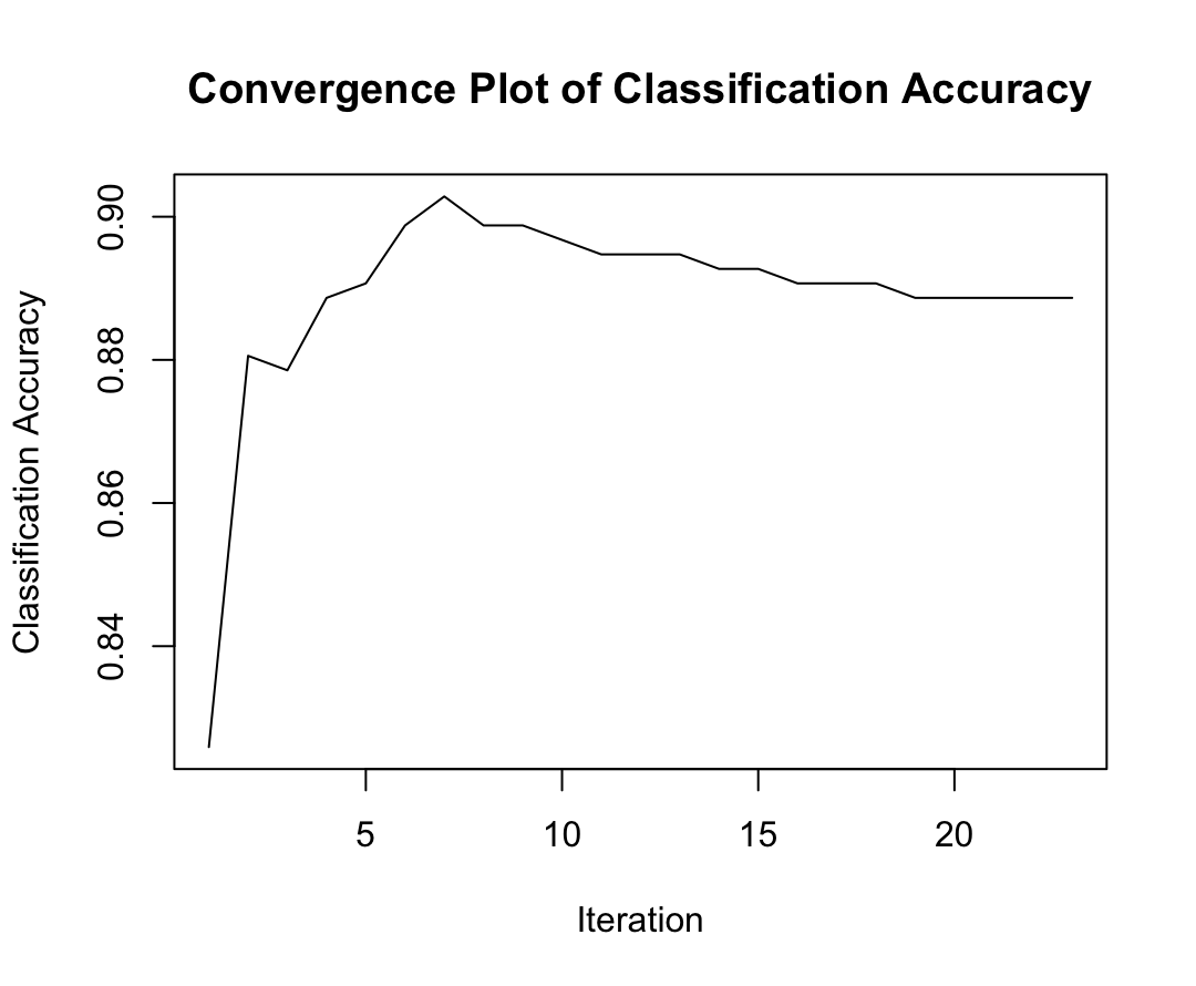


4.2.4 Initial Values
According to the results in Figure 5, it can be found that the observed log-likelihood function is small when using Method 1 as the initial values method, and there is a large difference in the convergence results for each of the 1000 experiments. In contrast, when using Method 2 as the initial values method, although the values obtained in each experiment are slightly different, the difference between the values is not large, the convergence of the model fit is more stable, and the observed log-likelihood function can converge to a higher value. And when using Method 3, the values of the observed log-likelihood function obtained are higher than most of the experimental results of Method 2. This is because by using as a priori, the model can obtain as much information as possible from the labeled data at the very beginning.
From Table 5, it can be seen that the classification accuracy using Method 1 is significantly lower, with an average of 0.64, and the relative bias of the estimators is also higher, with a rate of change between 22.9 and 132. The standard deviation is also much higher compared to Method 2. For Method 2 and Method 3, both methods can obtain high classification accuracy with a mean value of 0.87, and the relative deviations of the estimated coefficients for both are also relatively small, ranging from 0.6 to 11.2 and 2.8 to 11.3, respectively. In terms of relative bias and classification accuracy, there is no significant difference between these two methods. In addition, for Method 1, the number of iterations is only 46, while for Methods 2 and 3, 1424 and 17 iterations can be obtained. This indicates that the initial values selection of Method 1 can quickly fall into a local optimum.
Therefore, it is suggested that the choice of using as a priori in the selection of the initial value of , or using multiple initial values and selecting from them the initial values that make the maximum of the likelihood function, are to try to avoid the influence of local maxima.

| Method 1 | Mean | SD | BIAS | Relative Bias |
|---|---|---|---|---|
| 0.32 | 0.093 | 1.32 | -1.320 | |
| 0.26 | 0.097 | -0.24 | -0.485 | |
| 0.44 | 0.082 | -2.56 | -0.855 | |
| 0.14 | 0.044 | -0.66 | -0.824 | |
| 1.54 | 0.050 | -0.46 | -0.229 | |
| 0.03 | 0.056 | 0.13 | -1.259 | |
| -1.70 | 0.058 | 1.31 | -0.435 | |
| 0.04 | 0.031 | -0.16 | -0.777 | |
| 0.315 | 0.010 | 0.015 | ||
| Classification Accuracy | 0.64 | 0.020 | ||
| Method 2 | Mean | SD | BIAS | Relative Bias |
| -0.96 | 0.018 | 0.04 | -0.042 | |
| 0.50 | 0.014 | 0 | 0.006 | |
| 3.04 | 0.021 | 0.04 | 0.013 | |
| 0.76 | 0.010 | -0.04 | -0.049 | |
| 2.20 | 0.010 | 0.20 | 0.101 | |
| -0.11 | 0.006 | -0.009 | 0.091 | |
| -3.29 | 0.007 | -0.29 | 0.096 | |
| 0.22 | 0.003 | 0.022 | 0.112 | |
| 0.309 | 0.001 | 0.009 | ||
| Classification Accuracy | 0.87 | 0.004 | ||
| Method 3 | Mean | SD | BIAS | Relative Bias |
| -0.95 | – | 0.05 | -0.049 | |
| 0.51 | – | 0.01 | 0.028 | |
| 3.09 | – | 0.09 | -0.030 | |
| 0.77 | – | -0.03 | -0.037 | |
| 2.18 | – | 0.18 | 0.092 | |
| -0.11 | – | -0.01 | 0.091 | |
| -3.27 | – | -0.27 | 0.090 | |
| 0.22 | – | 0.02 | 0.113 | |
| 0.308 | – | 0.08 | ||
| Classification Accuracy | 0.87 | – |
5 Real Data Analyses
5.1 PRIME Trial
PRIME[68][69][70] is a randomized, multicenter Phase III trial, The objective of this study is to evaluate the efficacy and safety of the targeted agent panitumumab (a monoclonal antibody against epidermal growth factor receptor) in combination with chemotherapy agent FOLFOX4 (folinic acid, 5-fluorouracil, and oxaliplatin) in patients with metastatic colorectal cancer (mCRC).
The trial was conducted between 2006 and 2013 and enrolled 1183 previously untreated mCRC patients. As shown in Figure 6, 593 patients in the experimental group received panitumumab plus FOLFOX4, and 590 patients in the control group received FOLFOX4 alone. The trial also included an analysis of the relationship between treatment outcomes in two subgroups of patients with wild-type KRAS tumors and patients with KRAS-mutated tumors, respectively.KRAS is a gene that encodes a KRAS protein, which KRAS mutations are common in various types of cancer, including colorectal cancer. KRAS mutations and wild-type refer to the status of the KRAS gene in tumor cells of patients with metastatic colorectal cancer. KRAS mutations are genetic alterations that result in changes in the DNA sequence of the KRAS gene, resulting in the production of abnormal KRAS proteins. In contrast, wild-type KRAS refers to the normal, unaltered form of the KRAS gene. The primary endpoint of the trial is progression-free survival (PFS), with secondary endpoints including overall survival (OS), objective response rate (ORR), duration of response (DOR), and safety.
As shown in Figures 7,8 and tables 6 (Note: The public data set contains only of subjects, and the results are slightly different from those in the original paper), the results of the test taking KRAS status into account show that, progression-free survival is improved with the addition of panitumumab to chemotherapy versus chemotherapy alone in patients with wild-type KRAS tumors. Specifically, median progression-free survival is 9.73 months ( CI 9.33 to 11.37) in the group receiving panitumumab plus chemotherapy versus 9.33 months (95 confidence interval (CI) 7.80 to 11.10) in the group receiving chemotherapy alone. The hazard ratio (HR) is 0.84 (95 CI 0.69-1.02, p=0.07) with a log-rank test p-value of 0.06. However, the addition of panitumumab to chemotherapy does not significantly improve progression-free survival, as compared with chemotherapy alone, in patients with KRAS-mutated tumors. Median PFS is 7.47 months (95 CI 6.40 to 8.47) in the group receiving panitumumab plus chemotherapy versus 9.1 months (95 CI 7.80 to 10.03) in the group receiving chemotherapy alone, with a hazard ratio (HR) of 1.19 (95 CI 0.95 to 1.50, p=0.13), log-rank test p-value is 0.075. Thus, the difference between KRAS mutant and wild-type in the PRIME trial is related to the difference in response to panitumumab plus chemotherapy between the two groups. Patients with KRAS wild-type tumors have an improved risk with the addition of panitumumab, whereas patients with KRAS mutant tumors have an increased risk.
In summary, this trial helps establish panitumumab as an effective treatment option for patients with metastatic colorectal cancer, especially for patients with KRAS wild-type tumors, highlighting the potential benefit of targeted therapy in this patient population and that KRAS status may be a useful biomarker for predicting response to panitumumab in patients with metastatic colorectal cancer. Next, we, therefore, will consider 514 patients only with wild-type KRAS.
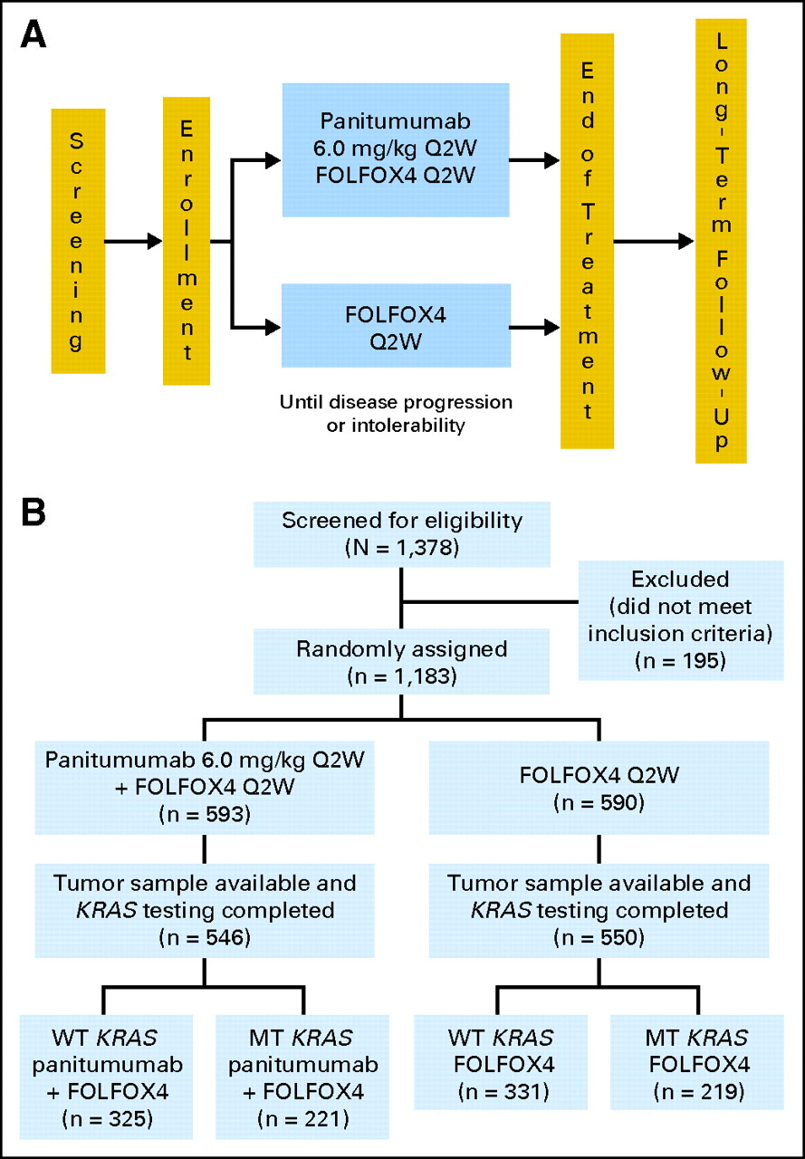


| Treatment | PFS | 95% CI Lower | 95% CI Upper |
|---|---|---|---|
| FOLFOX4 | 9.33 | 7.80 | 11.10 |
| Panitumumab–FOLFOX4 | 9.73 | 9.33 | 11.37 |
| Treatment | PFS | 95% CI Lower | 95% CI Upper |
|---|---|---|---|
| FOLFOX4 | 9.10 | 7.80 | 10.03 |
| Panitumumab–FOLFOX4 | 7.47 | 6.40 | 8.47 |
As shown in Table 8, the names, meanings, and taking values of baseline covariates after preprocessing of 514 cases of wild-type KRAS are given. To assess the impact of various baseline covariates on patient risk, a total of 9 baseline covariates were included: ATRT, ECOG, , SEX, , , DIAGTYPE, LIVERMET, LDH. The details are described below:
- 1.
Treatment modality (ATRT): Panitumumab + FOLFOX4 in the experimental group and FOLFOX4 in the control group.
- 2.
ECOG performance status (ECOG): The Eastern Cooperative Oncology Group (ECOG) performance status was used to assess the functional status of patients. Patients scoring 0-2 were included in the trial.ECOG performance status is a measure of a patient’s functional status and ability to perform daily activities.
- 3.
Metastatic burden (): The number of metastatic sites was analyzed as a potential prognostic factor.
- 4.
Gender (SEX): The patient’s gender was recorded in the study entry.
- 5.
Age (): The patient’s age was recorded at the time of study entry.
- 6.
Race (): The patient’s race was recorded at the time of study entry.
- 7.
Primary tumor location (DIAGTYPE): The location of the primary tumor in the colon or rectum was recorded.
- 8.
Presence or absence of metastasis to the liver at study entry (LIVERMET): The presence of liver metastasis is an important baseline covariate because it is a known prognostic factor in metastatic colorectal cancer and can affect treatment outcome.
- 9.
Baseline LDH (LDH): As a marker of tumor burden and prognosis. High LDH levels are associated with poorer prognosis in patients with metastatic colorectal cancer.
| Baseline covariates name | Meaning | Value ( percentage ) |
| 1=Panitumumab + FOLFOX4 | ||
| ATRT | experimental/control group | (experimental group 50.58) |
| 0=FOLFOX4(control group) | ||
| 1=Less than 50 of time in bed () | ||
| ECOG | Baseline ECOG status | 0=Fully active or |
| Symptomatic but movable people | ||
| SITESNUMSTRATA | Metastasis sites | 1=metastasis sites 3(44.16),0=others |
| SEX | Gender | 1=Male(64.01),0=Female |
| Age | 1=Age 65 (41.8),0= others | |
| White or not | 1= White or Caucasian(93.39),0=others | |
| DIAGTYPE | Primary tumor type | 1=Rectal(36.38), 0=Colon |
| LIVERMET | initial metastasis to the liver | 1=Yes(),0=NO |
| 1=LDH | ||
| LDH | Lactate dehydrogenase levels | 2ULN(29.18) |
| 0=LDH¡2ULN |
•
Model Algorithm Fitting
In the PRIME trial, the response of patients in the experimental group to the drugs was assessed according to the RECIST 1.1 criteria [60], and in the experimental group, we can estimate an objective response rate at . For the control group, we can not observe the drug’s response conditions in the control group because of the different mechanisms of action of the targeted drugs and chemotherapy, so in this subsection, we fit the Dual Cox model algorithm to 514 wild-type KRAS patients to classify the control group and explore the difference in the efficacy of panitumumab plus FOLFOX4 and FOLFOX4 alone on patients in different subgroups.
According to the Dual Cox model described in Section2, subsection 2, we randomly choose 1000 different initial values to fit the Dual Cox model, from which we select the initial values that make the maximum value of the log-likelihood function.
Finally, we obtain the form of the Dual Cox model as
the hazard function in the response group
the hazard function in the non-response group
where
•
Subgroup Classification
The Dual Cox model divides the unobserved population into the response and non-response groups, and the results are shown in Table 9. Among them, the response group contains 302 individuals with a censoring rate of 16.6, and the non-response group contains 212 individuals with a censoring rate of 18.4. The mean values of individual convergence probabilities in different populations are 0.95 and 0.98, respectively, which are close to 1, [[[indicating that the model can well converge individuals into the same subgroup, and there is little difference between individuals within the group]]]. In addition, as shown in Figure 9, the Dual Cox model algorithm is able to group the non-censored data well, and the maximum posterior probability is 1 for all non-censored data for the unobserved control population. However, for the censored data, the model has some uncertainty, but the certainty of classification increases with increasing progression-free survival, indicating that our algorithm has difficulty in classifying patients with censored, short progression-free survival, which is consistent with the conclusion of Eng and Hanlo[40]’s discussion about the unsupervised case. Based on the results of the subgroup classification, we can obtain an estimate of the objective response rate, which is 0.51 in the control group, compared to an estimated response rate of 0.61 in the experimental group, and the convergence results were in line with the real situation, that is, panitumumab plus FOLFOX4 can improve the objective response rate of patients in wild-type KRAS patients.
| Total Patients | Censored Rate() | Mean of | |
|---|---|---|---|
| Responders | 302 | 16.6 | 0.95 |
| Non-Responders | 212 | 18.4 | 0.98 |
| Overall Population | 514 | 17.3 | – |

•
Parameter Estimation
We fit the Cox proportional hazards model to the overall population and compare the results with the results of the Dual Cox Model. As shown in Table 10 and Figure 10, the estimated coefficients for the overall population, response, and non-response groups are all of the same sign for the eight baseline covariates except for treatment efficacy ATRT, which illustrates the homogeneity of the response and non-response groups for the eight baseline covariates except for ATRT and the heterogeneity for treatment efficacy ATRT.
For the overall population, ATRT is not significant at the level of 0.05 (p=0.07), and in the response group HR=0.1 with p-value ¡0.05, indicating better efficacy in the experimental group than in the control group for patients who have responded. In contrast, HR=3.52 with p-value¡0.05 in the non-response group, indicating better efficacy in the control group than in the experimental group for non-response patients; also, the estimated coefficients of baseline covariates ECOG and SITESNUMSTRATA, which are significant in both the responder group and overall population, show ECOG=1 (less than 50 of time in bed) and metastatic site3 have a significantly higher risk, but do not raise risk in the non-response group; also, for patients with age65 in the response group, the risk is significantly higher for age65, indicating that age65 has a higher risk for the response group, but not for the overall population, non-response group. For the overall population, non-responders group, there is no significant increase in risk. For the covariate LDH, LDH=1 shows a significantly higher risk than LDH=0 for the overall population, responders, and non-responders groups.
| Responders | Non-Responders | Overall Population | |||||||
|---|---|---|---|---|---|---|---|---|---|
| Covariates | HR | p-values | HR | p-values | HR | p-values | |||
| ATRT | -2.27 | 0.10 | 1.26 | 3.52 | -0.18 | 0.84 | 0.07 | ||
| ECOG | 0.99 | 2.68 | 0.53 | 1.69 | 0.16 | 0.50 | 1.64 | 0.02 | |
| SITES | 0.38 | 1.50 | 0.004 | 0.13 | 1.14 | 0.45 | 0.27 | 1.31 | 0.007 |
| SEX | -0.18 | 0.83 | 0.15 | -0.41 | 0.66 | 0.01 | -0.09 | 0.91 | 0.39 |
| AGE_65 | 0.34 | 1.40 | 0.01 | 0.06 | 1.06 | 0.74 | 0.11 | 1.11 | 0.30 |
| IS_WHITE | 0.06 | 1.06 | 0.81 | 0.30 | 1.35 | 0.31 | 0.08 | 1.08 | 0.70 |
| DIAGTYPE | -0.21 | 0.81 | 0.11 | -0.43 | 0.65 | 0.03 | -0.03 | 0.97 | 0.75 |
| LIVERMET | -0.54 | 0.58 | 0.004 | -0.29 | 0.75 | 0.19 | -0.24 | 0.78 | 0.12 |
| LDH | 0.53 | 1.70 | 0.53 | 1.70 | 0.004 | 0.34 | 1.40 | 0.001 | |
- 1
is indicated here by SITES
- 2
p-values below the significance level of 0.05 are indicated in bold

•
Diagnostics
After subgroup classifying, we fit Cox proportional hazards model in the response and non-response groups, respectively. After that, time-dependent ROC curve analysis is performed on the two subgroups and the overall population. Time-dependent ROC curve analysis is widely used in biomedical research to assess the performance of models [71].
Various definitions and estimation methods have been proposed in several literatures on time-dependent ROC curves [71][72]. Here, based on the method proposed by Heagerty and Zheng(2005)[73], sensitivity is extended to incident sensitivity and specificity is extended to dynamic specificity, and then ROC curves are drawn. Incident sensitivity refers to the probability that an individual has a marker value greater than c among individuals experiencing an event at time t. Dynamic specificity refers to the probability that an individual has a marker value less than or equal to c among individuals without an event at time t. It is generally accepted that higher marker values are more indicative of disease. The performance of markers is assessed by the area under the ROC curve (AUC); the higher the AUC value, the better the model performance.
At each time point t, each individual is categorized as a case or control. For each patient , let be the time of disease event and be the marker value ( under the Cox proportional hazards model). The observed survival time is , , where is the censoring time, and let be the censoring indicator variable that takes the value 1 when the event (disease) occurs and 0 otherwise.
Therefore, the sensitivity, specificity, and the resulting are defined as
Denote the risk set as . , is the size of S(t). Hagerty and Zheng[73] proposed to make the following estimates under the assumption of proportional hazards.
Depending on the value of different c, the sensitivity, and specificity sequences at the same time point can be obtained, then the ROC curve can be drawn. Xu and O’Quigley [74] proved the consistency of sensitivity estimation. Since the specificity is an empirical distribution on S(t), the specificity is also consistent if the sample is unbiased [73].
From Figure 11, it can be seen that from 0 to 1000 days, for the response group, the AUC is approximately between 0.8 and 0.6. For the non-response group, the AUC is between 0.7 and 0.65, and for the overall population, it is consistently below 0.6. These illustrate that the Cox model fitted for both the response and non-response groups performs better than the Cox model without classifying the subgroup. Similarly, as seen in Figure 12, the AUC at day 100 was 0.8 for the response group, 0.7 for the non-response group, and 0.58 for the overall population, showing that our model can successfully split the population into two subgroups. In this dataset, the Dual Cox model outperforms the Cox proportional hazards model.
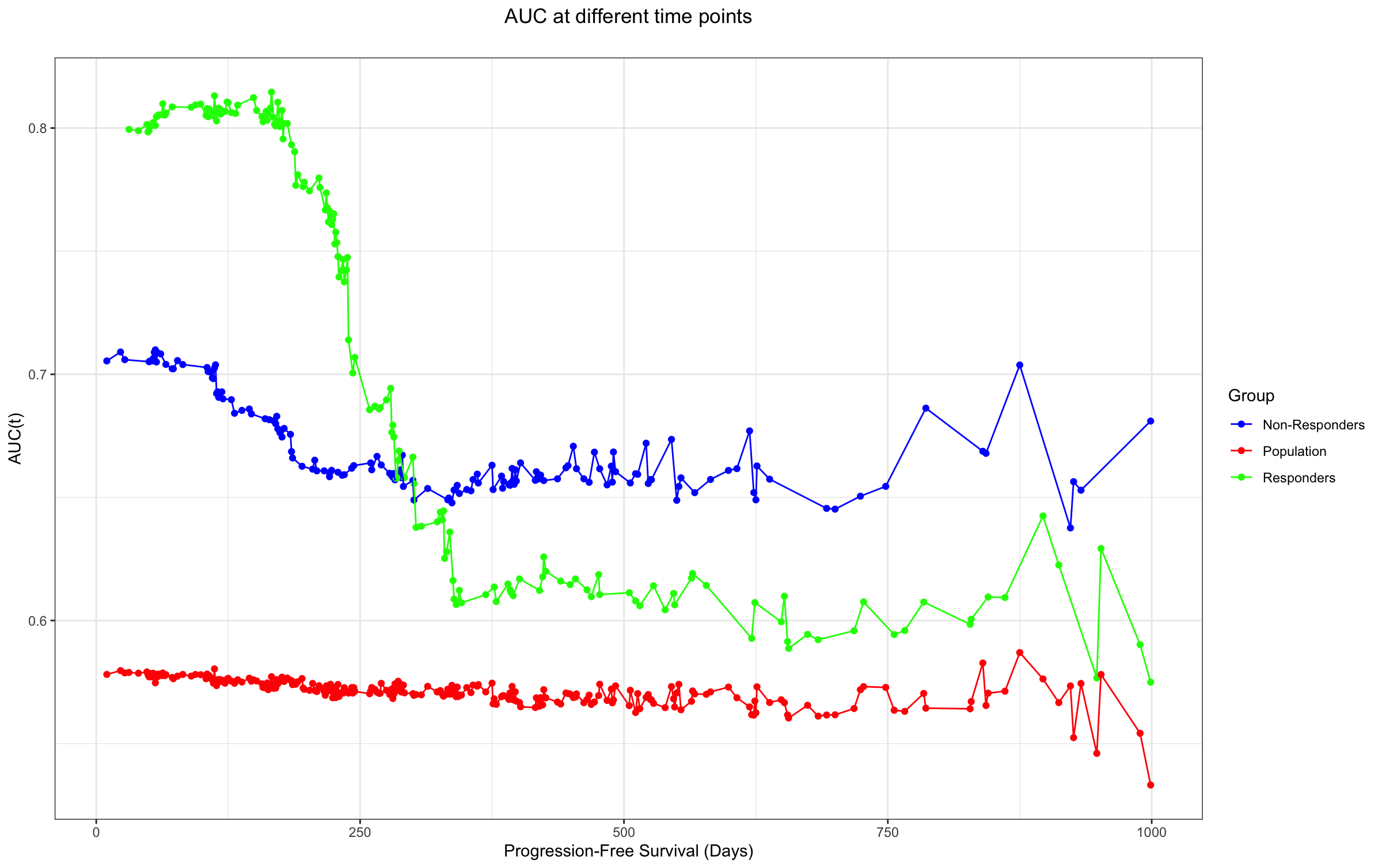
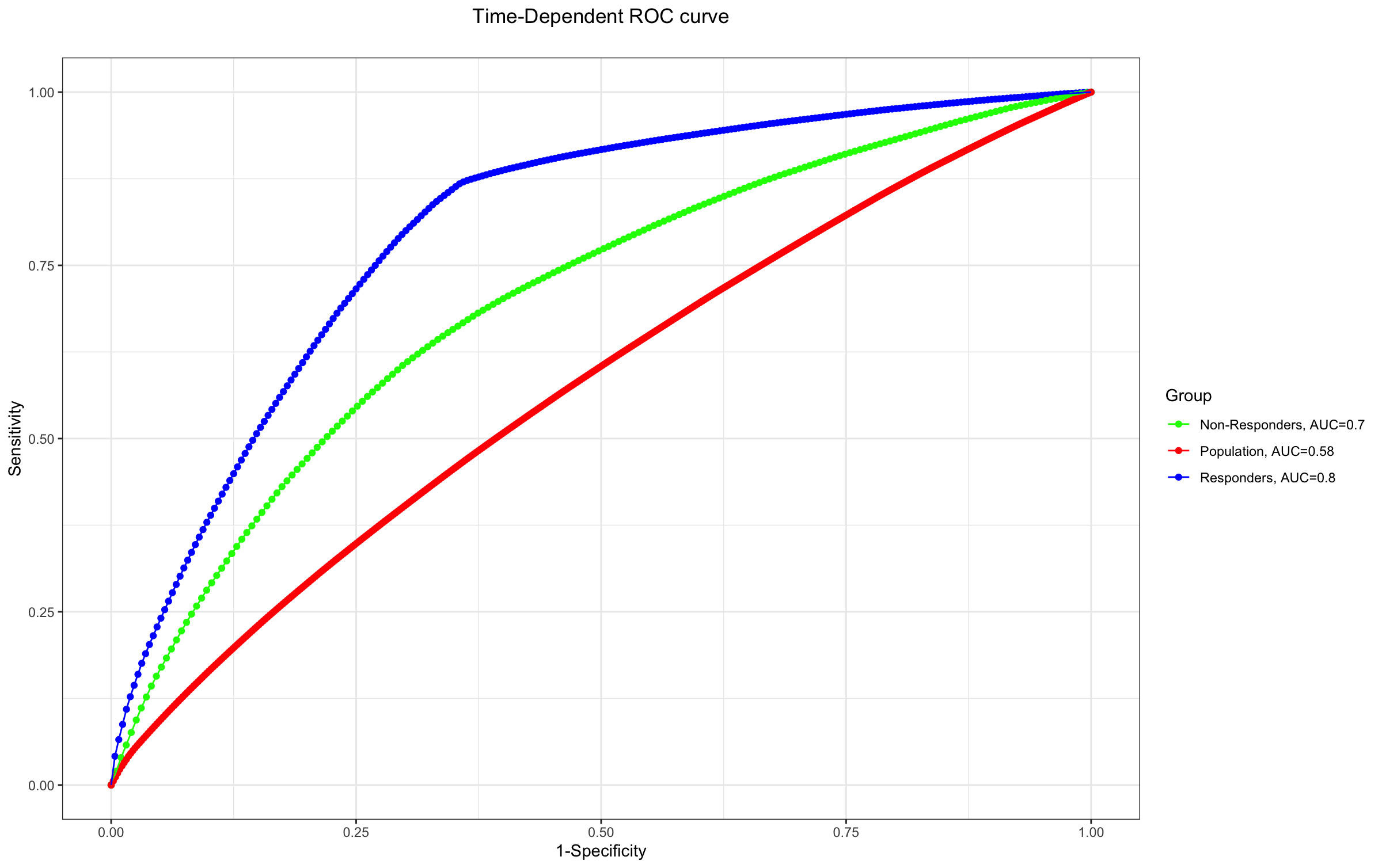
5.2 PACCE Trial
PACCE[75] is a randomized, open-label, multicenter phase IIIB clinical trial designed to evaluate the efficacy and safety of combining chemotherapy, bevacizumab (a humanized monoclonal antibody against tumor angiogenesis) and panitumumab (a monoclonal antibody against the epidermal growth factor receptor) and chemotherapy in combination with bevacizumab for the treatment of patients with metastatic colorectal cancer (mCRC). Based on investigator selection, patients were enrolled in one of two cohorts: a fluorouracil, folinic acid, and oxaliplatin-based chemotherapy (Ox-CT) cohort or a fluorouracil, folinic acid, and irinotecan-based chemotherapy (Iri-CT) cohort.
The study was conducted between 2005 and 2007, and as shown in Figure 13, 1053 patients were randomized to the study at 200 centers in the U.S. 823 were enrolled in the Ox-CT cohort and 230 were enrolled in the Iri-CT cohort. In both cohorts, patients were assigned in a 1:1 ratio to the experimental (bevacizumab and panitumumab) and control (bevacizumab) groups. The primary endpoint is progression-free survival (PFS), and secondary endpoints included overall survival (OS), objective response rate (ORR), and safety.
As shown in Figures 14, 15 and Tables 11, 12 (Note: The public data set contains only 80 of subjects, and the results are slightly different from those in the original paper), the trial results in the Ox-CT cohort shows that, compare to bevacizumab plus panitumumab, the use of bevacizumab alone improves progression-free survival in patients who receives bevacizumab compares to bevacizumab plus panitumumab.
Specifically, median progression-free survival is 10.93 months (95 CI 9.23-11.83) in the group receiving bevacizumab plus panitumumab compared with 12.10 months (95 CI 11.10-13.37) in the group receiving bevacizumab, with a hazard ratio (HR) of 1.18 (95 CI 0.99-1.40. P=0.07), log-rank test p-value of 0.096. However, the trial results at Iri-CT show no significant improvement in progression-free survival in patients on bevacizumab alone compared with bevacizumab added to panitumumab. The median progression-free survival is 12.43 months (95 CI 10.10-14.47) in the group receiving bevacizumab added to panitumumab compared to 11.87 months (95 CI 10.33-16.23) in the group receiving bevacizumab, with a hazard ratio (HR) of 1.09 (95 CI 0.74-1.61, p=0.66). The log-rank test p-value is 0.48. Thus, the difference between the Ox-CT cohort and the Iri-CT in the PACCE trial is related to the difference in response to the addition of panitumumab between the two groups. Patients with tumors in the Iri-CT cohort have no improvement in risk with the addition of panitumumab, whereas patients with tumors in the Ox-CT cohort have an increased risk.
In summary, the trial does not support the use of panitumumab in combination with bevacizumab and oxaliplatin or irinotecan-based chemotherapy for the treatment of metastatic colorectal cancer. There is no difference between the panitumumab in combination with bevacizumab group and the bevacizumab group in the Iri-CT cohort, and patients with panitumumab in combination with bevacizumab in the Ox-CT cohort perform worse in terms of progression-free survival. We therefore next consider only 653 patients in the Ox-CT cohort.

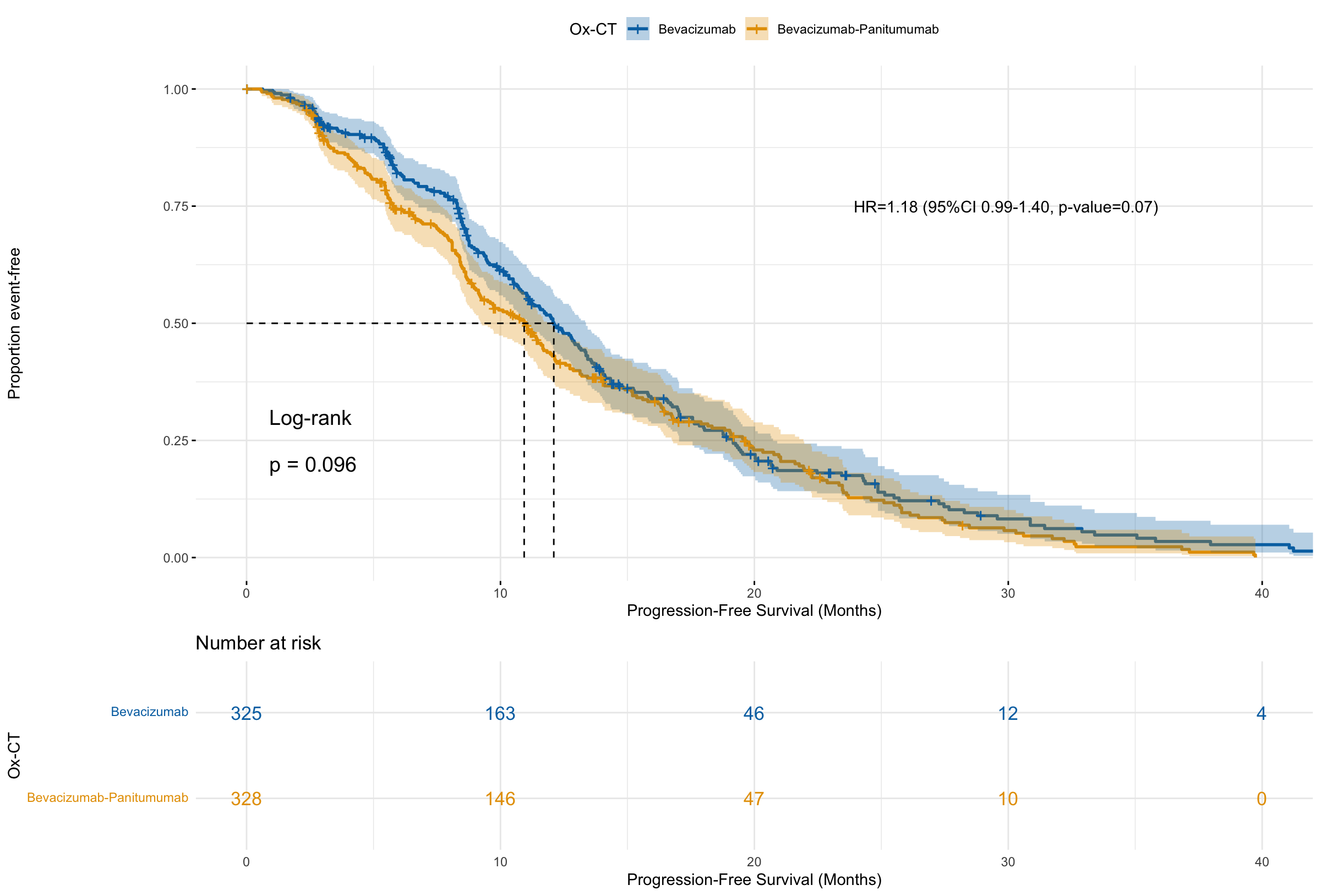
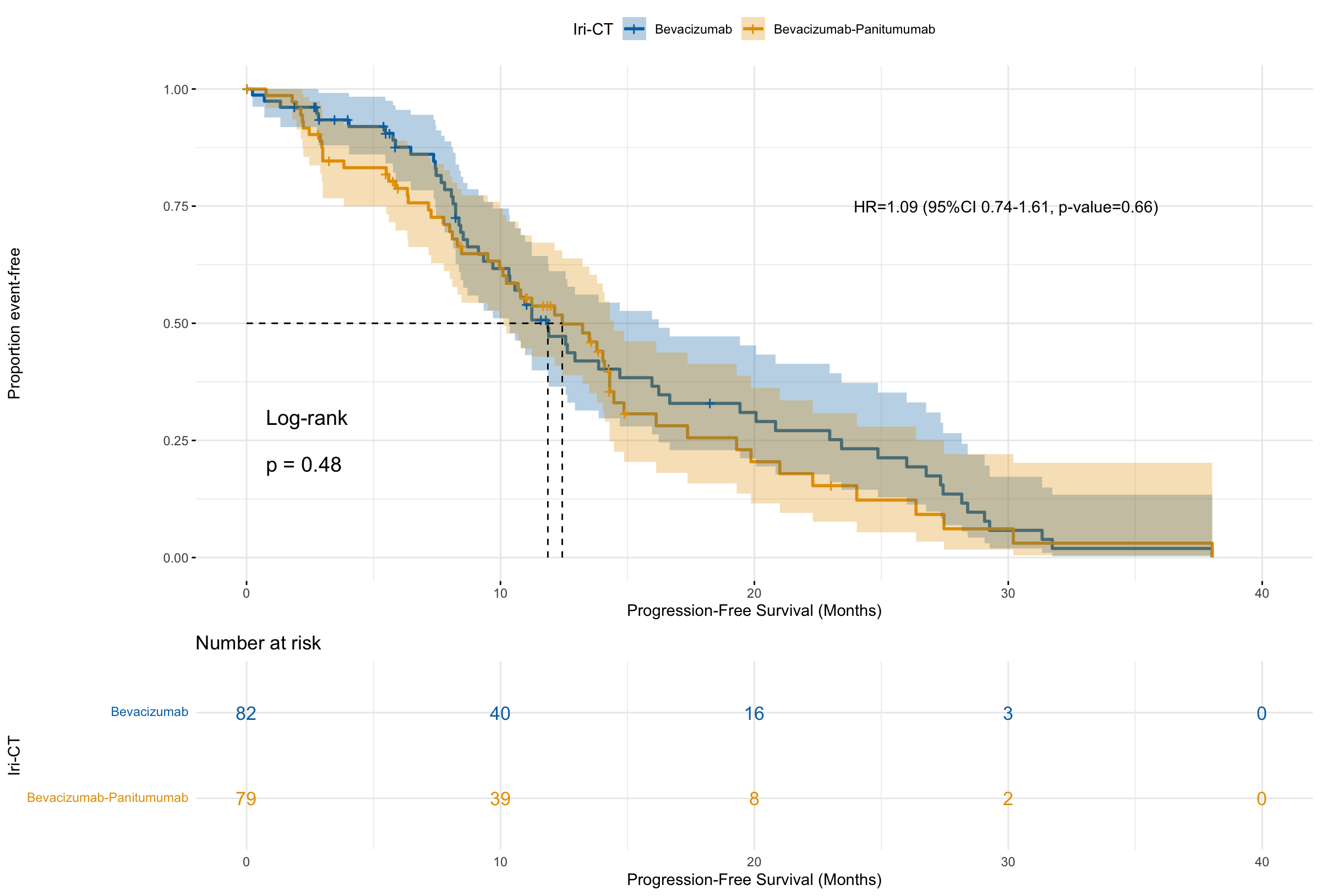
| Treatment | Progression-free Survival | 95% CI Lower | 95% CI Upper |
|---|---|---|---|
| Bevacizumab | 12.10 | 11.10 | 13.37 |
| Bevacizumab-Panitumumab | 10.93 | 9.23 | 11.83 |
| Treatment | Progression-free Survival | 95% CI Lower | 95% CI Upper |
|---|---|---|---|
| Bevacizumab | 11.87 | 10.33 | 16.23 |
| Bevacizumab-Panitumumab | 12.43 | 10.10 | 14.47 |
As shown in Table 13, the names, meanings, and values of the baseline covariates after preprocessing are given for 653 patients in the Ox-CT cohort. To assess the impact of various baseline covariates on patient risk, a total of 10 baseline covariates were included: ,, SEX, , , DIAGTYPE, LDH, KRASCD, and PRADJYN. The details are described below:
- 1.
Treatment modality (ATRT): Bevacizumab + FOLFOX4 in the experimental group and bevacizumab in the control group.
- 2.
ECOG performance status (ECOG): The Eastern Cooperative Oncology Group (ECOG) performance status was used to assess the functional status of patients. Patients scoring 0-2 were included in the trial. ECOG performance status is a measure of a patient’s functional status and ability to perform daily activities.
- 3.
Metastatic burden (): The number of metastatic sites was analyzed as a potential prognostic factor.
- 4.
Gender (SEX): The patient’s gender was recorded in the study entry.
- 5.
Age (): The patient’s age was recorded at the time of study entry.
- 6.
Race (): The patient’s race was recorded at the time of study entry.
- 7.
Primary tumor location (DIAGTYPE): The location of the primary tumor in the colon or rectum was recorded.
- 8.
Baseline LDH (LDH): As a marker of tumor burden and prognosis. High LDH levels are associated with poorer prognosis in patients with metastatic colorectal cancer.
- 9.
KRAS gene (KRASCD): KRAS gene is a useful biomarker for predicting response to panitumumab.
- 10.
Adjuvant therapy (PRADJYN): Records whether the patient has had adjuvant therapy.
| Baseline covariates name | Meaning | Value ( percentage ) |
| 1 = Bevacizumab +Panitumumab | ||
| ATRT | Experimental/control group | (experimental group 49) |
| 0=FOLFOX4(control group) | ||
| 1=Less than 50 of time in bed () | ||
| ECOG | Baseline ECOG status | 0=Fully active or |
| Symptomatic but movable people | ||
| SITESNUMSTRATA | Metastasis sites | 1=metastasis sites 3(21.7),0=others |
| SEX | Gender | 1=Male(55.3),0=Female |
| Age | 1=Age 65 (34.8),0= others | |
| White or not | 1= White or Caucasian(72.7),0=others | |
| DIAGTYPE | Primary tumor type | 1=Rectal(21.7), 0=Colon |
| 1=LDH | ||
| LDH | Lactate dehydrogenase levels | 1.5ULN(18.6) |
| 0=LDH¡1.5ULN | ||
| 1=Wild type() | ||
| KRASCD | KRAS Gene Results | 2=Mutant type() |
| 88=Failure | ||
| PRADJYN | Adjuvant treatment | 1=Yes(),0=NO |
•
Model Fitting
In the PACCE trial, we estimate an objective response rate of 0.45 in the experimental group, which was assessed according to mRECIST criteria [61]. In this subsection, we fit the Dual Cox model to the 672 patients in the Ox-CT cohort, classified the control population in the Ox-CT cohort, and investigated the effect of panitumumab plus Bevacizumab as compared with Bevacizumab alone.
Similar to the previous subsection 5.1.1 for the PRIME dataset, we randomly choose 1000 different initial values to fit the Dual Cox model algorithm, from which we select the initial value that make the maximum value of the log-likelihood function.
Finally, we obtain the form of the the Dual Cox model as
the hazard function in the response group
the hazard function in the non-response group
where
•
Subgroup Classification
The Dual Cox model divides the unobserved population into two groups, responders and non-responders, and the results are shown in Table 14. The response group contains 348 individuals with a censoring rate of 17.0, and the non-response group contains 305 individuals with a censoring rate of 31.8. The mean values of individual convergence probabilities in different subgroups are 0.96 and 0.96, respectively, which are close to 1, indicating that the model can well converge individuals into the same subgroup, and there is little difference between individuals within the group. In addition, as shown in Figure 16, the Dual Cox model can classify the non-censored data well, and the maximum posterior probability is 1 for all non-censored data for the unobserved control group. However, for the censored data, the model has some uncertainty in classifying patients, but the certainty of classification increases as the progression-free survival increases, suggesting that our algorithm has difficulty classifying patients with censored and short progression-free survival. These conclusions for the convergence results are consistent with those of the previous subsection for the PRIME dataset. Based on the subgroup classification results, the objective response rate of 0.61 is estimated for the control group, compared to an estimated response rate of 0.45 in the experimental group, and the convergence results are consistent with the true situation, i.e., the response rate of patients with panitumumab combined with bevacizumab in the Ox-CT cohort is worse than that of bevacizumab.
| Total Patients | Censored Rate() | Mean of | |
|---|---|---|---|
| Responders | 348 | 17.0 | 0.96 |
| Non-Responders | 305 | 31.8 | 0.96 |
| Overall Population | 653 | 23.9 | – |

•
Parameter Estimation
We fit the Cox proportional hazards model to the overall population and compare the results with those based on the Dual Cox Model. As shown in Table 15 and Figure 17, for the overall, response, and non-response groups on treatment efficacy ATRT, the hazard ratio is 0.21 for the response group and 5.26 for the non-response group, and the p-values for both response and non-response groups are less than the significance level of 0.05, indicating the responding and non-responding populations on treatment efficacy heterogeneity in ATRT; some of the baseline covariates have the same effect on the population in the overall, responder, and non-responder groups, e.g., the estimated regression coefficients signs of the six baseline covariates ECOG, SITES, SEX, DIAGTYPE, LDH, and KRASCD are the same. For the baseline covariate ECOG (1=less than 50 of time in bed, 0=fully active or symptomatic but mobile), it is significant in all three groups and has the same sign in all three groups, showing that ECOG=1 had a significantly higher risk than ECOG=0, which is in line with our perception that bedridden people are at greater risk; also, for example, for age 65 years old or with metastatic site number 3 or primary tumor type of rectum, the risk is significantly higher in the response and overall groups, but not in the non-response group, suggesting that age 65 years old, metastatic site number 3 or primary tumor type of rectum in the non-response group does not raise the risk of patients. For the effect of the covariate SEX, it can be found that only the response group has an effect on risk, while in the overall and non-response groups, there is no effect on patients’ progression-free survival; for KRASCD, PRADJYN, LDH, and , they are non-significant in all three groups, which means that in all three groups, these baseline covariates do not have an impact on patient risk in any of the three groups.
| Responders | Non-Responders | Overall Population | |||||||
| Covariates | HR | p-values | HR | p-values | HR | p-values | |||
| ATRT | -1.58 | 0.21 | 1.66 | 5.26 | 0.16 | 1.18 | 0.07 | ||
| ECOG | 0.73 | 2.07 | 0.61 | 1.85 | 0.31 | 1.37 | |||
| SITES | 0.47 | 1.60 | 0.004 | 0.07 | 1.08 | 0.71 | 0.30 | 1.35 | 0.01 |
| SEX | -0.54 | 0.58 | -0.10 | 0.91 | 0.51 | -0.04 | 0.96 | 0.64 | |
| AGE_65 | 0.32 | 1.38 | 0.01 | -0.01 | 0.99 | 0.95 | 0.21 | 1.23 | 0.02 |
| IS_WHITE | -0.11 | 0.89 | 0.81 | 0.30 | 1.35 | 0.14 | 0.10 | 1.10 | 0.45 |
| DIAGTYPE | 0.30 | 1.35 | 0.05 | 0.14 | 1.15 | 0.43 | 0.24 | 1.27 | 0.03 |
| LDH | 0.22 | 1.25 | 0.15 | 0.18 | 1.20 | 0.29 | 0.03 | 1.03 | 0.81 |
| KRASCD | 0 | 1.00 | 0.98 | 0 | 1.00 | 0.16 | 0 | 1.00 | 0.33 |
| PRADJYN | 0.10 | 1.11 | 0.58 | -0.14 | 0.87 | 0.44 | 0.06 | 1.06 | 0.63 |
- 1
is indicated here by SITES
- 2
p-values below the significance level of 0.05 are indicated in bold

•
Diagnostics
As in section 5.1.1 for the PRIME data, to assess the performance of the model, after classifying the subgroup, we fit three separate Cox proportional hazards models for the responders, non-responders, and the overall population, after which time-dependent ROC curves are analyzed.
From Figure 18, it can be seen that from 0 to 900 days, for the response group, the AUC is approximately between 0.75 and 0.55. For the non-response group, the AUC is between 0.75 and 0.68, and for the overall population it is consistently below 0.6. These illustrate that the Cox model fitted for both the response and non-response groups performs better than the unclassified population, meaning that the Dual Cox model is better. In addition, it can be found that for the response group, the AUC decreases gradually after 250 days. To better illustrate that our model performs better than fitting the Cox proportional hazards model alone, we give the ROC curves for the three populations at day 100, and from Figure 19, we can see that the AUC at day 100 is 0.73 for the response group, 0.72 for the non-response group, and 0.57 overall, all of which indicate that our model can effectively classify the subgroup, and the Dual Cox model fitted to the corresponding group have higher model performance compared to the overall population.
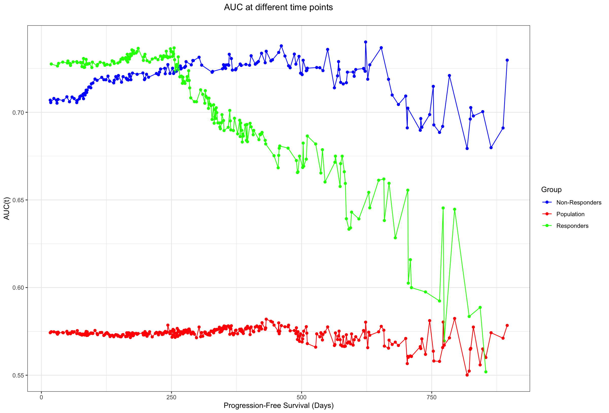
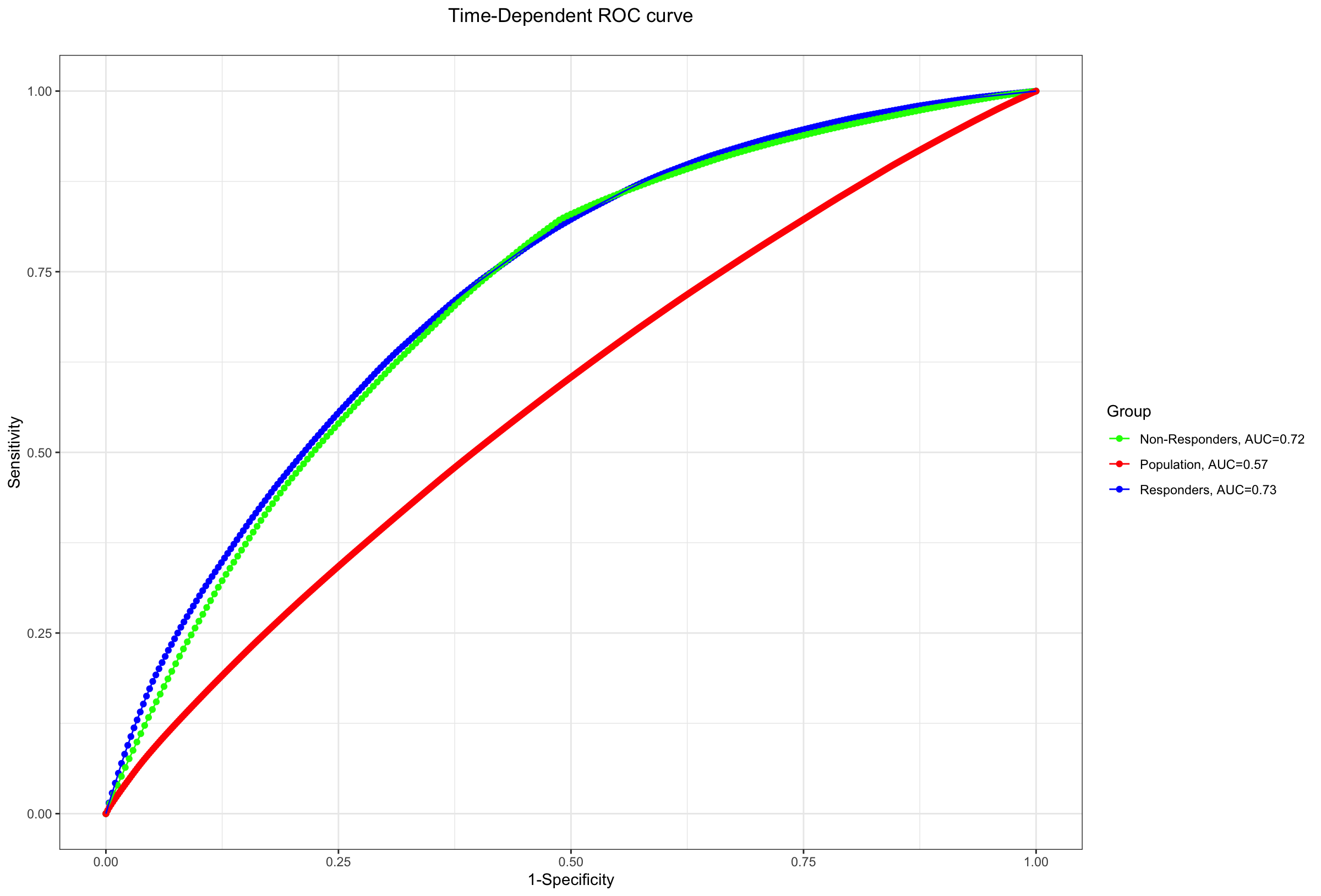
6 Conclusion and Discussion
6.1 Conclusion
Targeted therapy and immunotherapy differ significantly from conventional cancer treatment. Cox proportional hazards models may not be as effective when long-term survival and delayed clinical effects occur due to individual differences in drug response. Since the innovative cancer treatment and the control treatment have such distinct mechanisms of action, we can only observe responses in the experimental group. These considerations prompt us to investigate a semi-supervised model that would classify patients in the control group into responders and non-responders, thereby reducing the number of samples and time required to complete clinical trials and lowering research and development expenses. In other words, we can predict how the control population will respond to the medicine and restrict the assumption of proportional hazards to just the responders and non-responders. Finally, we analyzed the drug’s effectiveness by modeling both the responders and the non-responders simultaneously. The Dual Cox Model is therefore what we advocate for.
For the fitting of the Dual Cox model, as with the general finite mixture model, the semi-supervised mixture Cox model uses the EM algorithm to calculate the posterior probabilities of individuals belonging to the response and non-response groups by the E step, updates the mixing probabilities by the M step, and estimates the regression coefficients by maximizing partial likelihood function in the weighted Cox proportional hazards model. The algorithm iterates until the log-likelihood function converges by successive iterations.
This paper expands on the work of Anderson and Gill (1982)[43] and You et al. (2018)[42] to further show that our model has estimators with consistency and asymptotic normality, proving the validity of the Dual Cox model with large samples. A series of simulation tests are carried out in this study to confirm the validity of the model fit further once the theoretical properties are guaranteed. We first investigate the impact of various initial values selections on the model’s convergence outcomes. The results of the experiments demonstrate that the method will converge to a local maximum if the initial values are chosen on the boundary, thus leading to unguaranteed convergence. In contrast, the initial values chosen away from the boundary can produce better convergence outcomes. The impact of various sample sizes and censoring rates on the efficacy of the model is then covered. The experimental findings demonstrate that our approach has high classification accuracy and can guarantee unbiased parameter estimation. The stability is assured with 1000 repetitions of an experiment with minor variance.
To demonstrate the utility of the Dual Cox model theory in oncology clinical trials, we select the PRIME and PACCE trial datasets. For the subgroup classification problem, the Dual Cox model shows good ability to classify non-censored data accurately, but there is some uncertainty for the classification of censored data. However, the certainty of classification gradually improves with increasing progression-free survival. In estimating the objective response rate in the control group, the model can better reflect the actual situation. In addition, the model can effectively demonstrate heterogeneity in the drug’s efficacy in estimating regression coefficients and are consistent with our knowledge of the homogeneity of other baseline covariates. Finally, we use the diagnostics to demonstrate that the Dual Cox model outperforms the Cox proportional hazards model adapted to the overall population at various time points.
6.2 Discussion
Finite mixture models usually assume that each subgroup has a separate distribution to deal with heterogeneity among subgroups. Although the Cox proportional hazards model has become the most popular regression model applicable to censored time, its non-parametric properties make the construction of a Cox model with a finite mixture more challenging[42]. Therefore, Eng and Hanlon (2014)[40] proposed an algorithm to fit a finite mixture Cox model. Our proposed Dual Cox model serves as an extension of the finite mixture Cox model, whose main concern is to classify patients into responders’ and non-responders’ groups, thus fixing the number of subgroups to 2. In addition, a semi-supervised mixture Cox model is necessary to take into account some of the patients for whom a medication response has been observed. The distributions selected in the finite mixture model can be those used in common survival analyses in addition to the Cox proportional hazards model to characterize different subgroups of hazards, including Log-normal distribution, Weibull distribution, Gamma distribution, etc.[32][30]. Similar to our work, a mixture model based on these distributions can be extended to the semi-supervised case and compared with the Dual Cox model, which can help us better to assess the merits of the Dual Cox model.
The setting of the number of subgroups of the finite mixture Cox model generally needs to be set in advance, and the number of subgroups and the selection of initial values may lead to unstable convergence results of the EM algorithm, thus posing a challenge to the analysis. Compared with this, the advantage of the Dual Cox model is that the number of fixed groups is two, which are the responses’ group and the non-responders’ group, and the convergence result of its algorithm is more stable than that of the mixture Cox model with multiple groups.
The reasonableness of the estimation has been shown in Section 3, but the strict concavity of the likelihood function is based on the assumption of regularity conditions. Therefore, after fitting using the EM algorithm, there is no guarantee that the likelihood function of the Dual Cox model necessarily converges to a global maximum. In our experiments, with a 1:1 ratio of labeled to unlabeled data, the log-likelihood function converges to higher values well enough to achieve high classification accuracy and ensure consistency and asymptotic normality in the estimated coefficients, as long as we avoid the choice of initial values in the boundary. To mitigate the effect of initial values, in addition to using the EM algorithm, Ueda and Nakano (1998)[76] proposed using the deterministic annealing EM algorithm, while Celeux, Chauveau, and Diebolt (1996)[77] proposed a stochastic EM algorithm, all of these techniques seek to allow the EM algorithm to iterate from less-than-ideal initial values and converge to better results. Consequently, we will consider how to appropriately modify the algorithm for the Dual Cox model in the future.
With the increase in data collection and baseline covariates, variable selection becomes an effective method for selecting risk factors. The importance of variable selection is particularly highlighted when there are many baseline covariates or even when the number of variables is larger than the sample size. The variables that are statistically significantly different for the three groups, the response group, the non-response group, and the overall population, are also different, so a model that allows variable selection on different subgroups becomes especially necessary. Tibshirani (1997)[78] proposed the use of LASSO on a Cox proportional hazards model with penalty term, Fan and Li (2002)[79] used SCAD penalty term on Cox proportional hazards model, You et al. (2018)[42] used adaptive LASSO penalty term on finite mixture Cox model. Thus, the Dual Cox model can be easily extended to include the use of variable selection methods to identify risk factors. By selecting variables, a better understanding of risk factors in different groups can be achieved, providing stronger evidence for clinical decision-making.
After determining the optimal subgroup, an important step is to evaluate its actual effects. Although statistical inference is usually used to analyze the selected subgroups, we must note that the subgroups may not be completely independent of the data selection. This may lead to an overly optimistic evaluation of the selected subgroups, which may influence our judgment of the treatment effect [80]. In addition, the lack of ability to detect treatment effects in smaller patient populations may produce false-positive results, which is particularly important because most clinical trials are designed to initially test treatment effects on the entire study population [81]. Thus, the Dual Cox model algorithm’s fitting results concerning subgroup classification may be biased. To reduce this bias, we need to adopt an approach to minimize the impact of false-positive results on the evaluation of treatment effects and provide more accurate individualized treatment plans to achieve the best results averaged over the entire patient population [82]. This will also be an essential research direction in our future work.
Acknowledgments
This was supported in part by the Fundamental Research Funds for the Central Universities, Sun Yat-sen University (Grant No. 20lgpy145 & 2021qntd21) and the Science and Technology Program of Guangzhou Project, Fundamental and Applied Research Project (202102080175).
References
- [1] Lynda Wyld, Riccardo A. Audisio, and Graeme J. Poston. The evolution of cancer surgery and future perspectives. Nature Reviews Clinical Oncology, 12(2):115–124, 2015.
- [2] John C. Warren. Inhalation of Ethereal Vapor for the Prevention of Pain in Surgical Operations. The Boston Medical and Surgical Journal, 35(19):375–379, 1846.
- [3] Joseph Lister. On the antiseptic principle in the practice of surgery. British medical journal, 2(351):246, 1867.
- [4] Vincent T. DeVita and Steven A. Rosenberg. Two Hundred Years of Cancer Research. New England Journal of Medicine, 366(23):2207–2214, 2012.
- [5] R. J. Papac. Origins of cancer therapy. The Yale Journal of Biology and Medicine, 74(6):391–398, 2001.
- [6] Serena Gianfaldoni, Roberto Gianfaldoni, Uwe Wollina, Jacopo Lotti, Georgi Tchernev, and Torello Lotti. An overview on radiotherapy: from its history to its current applications in dermatology. Open access Macedonian journal of medical sciences, 5(4):521, 2017.
- [7] Vincent T DeVita Jr and Edward Chu. A history of cancer chemotherapy. Cancer research, 68(21):8643–8653, 2008.
- [8] Muhammad T. Amjad, Anusha Chidharla, and Anup Kasi. Cancer Chemotherapy. In StatPearls. StatPearls Publishing, Treasure Island (FL), 2022.
- [9] G. Köhler and C. Milstein. Continuous cultures of fused cells secreting antibody of predefined specificity. Nature, 256(5517):495–497, 1975.
- [10] Viswanadha Vijaya Padma. An overview of targeted cancer therapy. BioMedicine, 5:1–6, 2015.
- [11] Yeuan Ting Lee, Yi Jer Tan, and Chern Ein Oon. Molecular targeted therapy: Treating cancer with specificity. European Journal of Pharmacology, 834:188–196, 2018.
- [12] Han-Chung Wu, De-Kuan Chang, and Chia-Ting Huang. Targeted therapy for cancer. J Cancer Mol, 2(2):57–66, 2006.
- [13] Ian D Davis. An overview of cancer immunotherapy. Immunology and Cell Biology, 78(3):179–195, 2000.
- [14] Shivani Srivastava and Stanley R. Riddell. Engineering CAR-T cells: Design concepts. Trends in Immunology, 36(8):494–502, 2015.
- [15] J. Joseph Melenhorst, Gregory M. Chen, Meng Wang, David L. Porter, Changya Chen, McKensie A. Collins, Peng Gao, Shovik Bandyopadhyay, Hongxing Sun, Ziran Zhao, Stefan Lundh, Iulian Pruteanu-Malinici, Christopher L. Nobles, Sayantan Maji, Noelle V. Frey, Saar I. Gill, Alison W. Loren, Lifeng Tian, Irina Kulikovskaya, Minnal Gupta, David E. Ambrose, Megan M. Davis, Joseph A. Fraietta, Jennifer L. Brogdon, Regina M. Young, Anne Chew, Bruce L. Levine, Donald L. Siegel, Cécile Alanio, E. John Wherry, Frederic D. Bushman, Simon F. Lacey, Kai Tan, and Carl H. June. Decade-long leukaemia remissions with persistence of CD4+ CAR T cells. Nature, 602(7897):503–509, 2022.
- [16] Tai-Tsang Chen. Statistical issues and challenges in immuno-oncology. Journal for ImmunoTherapy of Cancer, 1(1):18, 2013.
- [17] Raju R Raval, Andrew B Sharabi, Amanda J Walker, Charles G Drake, and Padmanee Sharma. Tumor immunology and cancer immunotherapy: summary of the 2013 SITC primer. Journal for ImmunoTherapy of Cancer, 2(1):14, 2014.
- [18] Kathleen M. Mahoney, Gordon J. Freeman, and David F. McDermott. The Next Immune-Checkpoint Inhibitors: PD-1/PD-L1 Blockade in Melanoma. Clinical Therapeutics, 37(4):764–782, 2015.
- [19] Alex D. Waldman, Jill M. Fritz, and Michael J. Lenardo. A guide to cancer immunotherapy: from T cell basic science to clinical practice. Nature Reviews Immunology, 20(11):651–668, 2020.
- [20] Luca Falzone, Salvatore Salomone, and Massimo Libra. Evolution of Cancer Pharmacological Treatments at the Turn of the Third Millennium. Frontiers in Pharmacology, 9:1300, 2018.
- [21] L.A. Renfro and D.J. Sargent. Statistical controversies in clinical research: basket trials, umbrella trials, and other master protocols: a review and examples. Annals of Oncology, 28(1):34–43, 2017.
- [22] Daniel V.T. Catenacci. Next-generation clinical trials: Novel strategies to address the challenge of tumor molecular heterogeneity. Molecular Oncology, 9(5):967–996, 2015.
- [23] E. L. Kaplan and Paul Meier. Nonparametric Estimation from Incomplete Observations. Journal of the American Statistical Association, 53(282):457–481, 1958.
- [24] J Martin Bland and Douglas G Altman. The logrank test. Bmj, 328(7447):1073, 2004.
- [25] D. R. Cox. Regression Models and Life-Tables. Journal of the Royal Statistical Society: Series B (Methodological), 34(2):187–202, 1972.
- [26] Jason J.Z. Liao and Guanghan Frank Liu. A flexible parametric survival model for fitting time to event data in clinical trials. Pharmaceutical Statistics, 18(5):555–567, 2019.
- [27] John D. Kalbfleisch and Ross L. Prentice. Estimation of the average hazard ratio. Biometrika, 68(1):105–112, 1981.
- [28] John W Boag. Maximum likelihood estimates of the proportion of patients cured by cancer therapy. Journal of the Royal Statistical Society. Series B (Methodological), 11(1):15–53, 1949.
- [29] Alexander D Tsodikov, Andrei Yu Yakovlev, and B Asselain. Stochastic models of tumor latency and their biostatistical applications, volume 1. World Scientific, 1996.
- [30] Gj McLachlan and Dc McGiffin. On the role of finite mixture models in survival analysis. Statistical Methods in Medical Research, 3(3):211–226, 1994.
- [31] Geoffrey McLachlan and David Peel. Finite Mixture Models: McLachlan/Finite Mixture Models. Wiley Series in Probability and Statistics. John Wiley & Sons, Inc., Hoboken, NJ, USA, 2000.
- [32] Ulku Erisoglu, Murat Erisoglu, and Hamza Erol. Pak. j. statist. 2012 vol. 28 (1), 115-130 mixture model approach to the analysis of heterogeneous survival data. Pak. J. Statist, 28(1):115–130, 2012.
- [33] Guanghan Frank Liu and Jason J. Z. Liao. Analysis of time-to-event data using a flexible mixture model under a constraint of proportional hazards. Journal of Biopharmaceutical Statistics, 30(5):783–796, 2020.
- [34] Beilin Jia, Donglin Zeng, Jason J. Z. Liao, Guanghan F. Liu, Xianming Tan, Guoqing Diao, and Joseph G. Ibrahim. Inferring latent heterogeneity using many feature variables supervised by survival outcome. Statistics in Medicine, 40(13):3181–3195, 2021.
- [35] Chi Wang. An Exponential Tilt Mixture Model for Time-to-Event Data to Evaluate Treatment Effect Heterogeneity in Randomized Clinical Trials. Biometrics & Biostatistics International Journal, 1(2), 2014.
- [36] Jing Qin. Empirical Likelihood Ratio Based Confidence Intervals for Mixture Proportions. The Annals of Statistics, 27(4):1368–1384, 1999. Publisher: Institute of Mathematical Statistics.
- [37] F. Zou. On empirical likelihood for a semiparametric mixture model. Biometrika, 89(1):61–75, 2002.
- [38] Ori Rosen and Martin Tanner. Mixtures of proportional hazards regression models. Statistics in Medicine, 18(9):1119–1131, 1999.
- [39] Ruo-fan Wu, Ming Zheng, and Wen Yu. Subgroup Analysis with Time-to-Event Data Under a Logistic-Cox Mixture Model: Subgroup analysis with censored data. Scandinavian Journal of Statistics, 43(3):863–878, 2016.
- [40] Kevin H. Eng and Bret M. Hanlon. Discrete mixture modeling to address genetic heterogeneity in time-to-event regression. Bioinformatics, 30(12):1690–1697, February 2014. _eprint: https://academic.oup.com/bioinformatics/article-pdf/30/12/1690/48926918/bioinformatics_30_12_1690.pdf.
- [41] A. P. Dempster, N. M. Laird, and D. B. Rubin. Maximum Likelihood from Incomplete Data Via the EM Algorithm. Journal of the Royal Statistical Society: Series B (Methodological), 39(1):1–22, 1977.
- [42] Na You, Shun He, Xueqin Wang, Junxian Zhu, and Heping Zhang. Subtype classification and heterogeneous prognosis model construction in precision medicine. Biometrics, 74(3):814–822, 2018.
- [43] Per Kragh Andersen and Richard D Gill. Cox’s regression model for counting processes: a large sample study. The annals of statistics, pages 1100–1120, 1982.
- [44] Mai Zhou. Understanding the Cox Regression Models With Time-Change Covariates. The American Statistician, 55(2):153–155, 2001.
- [45] Terry M Therneau, Patricia M Grambsch, Terry M Therneau, and Patricia M Grambsch. The cox model. Springer, 2000.
- [46] Terry M Therneau and Thomas Lumley. Package ‘survival’. R Top Doc, 128(10):28–33, 2015.
- [47] George YC Wong, Michael P Osborne, Qinggang Diao, and Qiqing Yu. Piecewise cox models with right-censored data. Communications in Statistics-Simulation and Computation, 46(10):7894–7908, 2017.
- [48] Joseph Berkson and Robert P Gage. Survival curve for cancer patients following treatment. Journal of the American Statistical Association, 47(259):501–515, 1952.
- [49] Paul C Lambert. Modeling of the cure fraction in survival studies. The Stata Journal, 7(3):351–375, 2007.
- [50] Federico Felizzi, Noman Paracha, Johannes Pöhlmann, and Joshua Ray. Mixture Cure Models in Oncology: A Tutorial and Practical Guidance. PharmacoEconomics - Open, 5(2):143–155, 2021.
- [51] Mailis Amico and Ingrid Van Keilegom. Cure models in survival analysis. Annual Review of Statistics and Its Application, 5:311–342, 2018.
- [52] Xiaoyu Jia, Camelia S. Sima, Murray F. Brennan, and Katherine S. Panageas. Cure models for the analysis of time-to-event data in cancer studies: Cure Models in Cancer Studies. Journal of Surgical Oncology, 108(6):342–347, 2013.
- [53] Judy P. Sy and Jeremy M. G. Taylor. Estimation in a Cox Proportional Hazards Cure Model. Biometrics, 56(1):227–236, 2000.
- [54] C. F. Jeff Wu. On the Convergence Properties of the EM Algorithm. The Annals of Statistics, 11(1), 1983.
- [55] Art B Owen. Empirical likelihood. CRC press, 2001.
- [56] Juan Shen and Xuming He. Inference for Subgroup Analysis With a Structured Logistic-Normal Mixture Model. Journal of the American Statistical Association, 110(509):303–312, 2015.
- [57] Norman E Breslow. Contribution to discussion of paper by dr cox. Journal of the Royal Statistical Society, Series B, 34:216–217, 1972.
- [58] World Health Organization et al. WHO handbook for reporting results of cancer treatment. World Health Organization, 1979.
- [59] Patrick Therasse, Susan G. Arbuck, Elizabeth A. Eisenhauer, Jantien Wanders, Richard S. Kaplan, Larry Rubinstein, Jaap Verweij, Martine Van Glabbeke, Allan T. van Oosterom, Michaele C. Christian, and Steve G. Gwyther. New Guidelines to Evaluate the Response to Treatment in Solid Tumors. JNCI: Journal of the National Cancer Institute, 92(3):205–216, 2000.
- [60] Elizabeth A Eisenhauer, Patrick Therasse, Jan Bogaerts, Lawrence H Schwartz, Danielle Sargent, Robert Ford, Janet Dancey, S Arbuck, Steve Gwyther, Margaret Mooney, et al. New response evaluation criteria in solid tumours: revised recist guideline (version 1.1). European journal of cancer, 45(2):228–247, 2009.
- [61] Riccardo Lencioni and Josep Llovet. Modified RECIST (mRECIST) Assessment for Hepatocellular Carcinoma. Seminars in Liver Disease, 30(01):052–060, 2010.
- [62] Haesun Choi, Chuslip Charnsangavej, Silvana C Faria, Homer A Macapinlac, Michael A Burgess, Shreyaskumar R Patel, Lei L Chen, Donald A Podoloff, and Robert S Benjamin. Correlation of computed tomography and positron emission tomography in patients with metastatic gastrointestinal stromal tumor treated at a single institution with imatinib mesylate: proposal of new computed tomography response criteria. Journal of clinical Oncology, 25(13):1753–1759, 2007.
- [63] Andrew Dennis Smith, Michael L Lieber, and Shetal N Shah. Assessing tumor response and detecting recurrence in metastatic renal cell carcinoma on targeted therapy: importance of size and attenuation on contrast-enhanced ct. American Journal of Roentgenology, 194(1):157–165, 2010.
- [64] Jedd D Wolchok, Axel Hoos, Steven O’Day, Jeffrey S Weber, Omid Hamid, Celeste Lebbé, Michele Maio, Michael Binder, Oliver Bohnsack, Geoffrey Nichol, et al. Guidelines for the evaluation of immune therapy activity in solid tumors: immune-related response criteria. Clinical cancer research, 15(23):7412–7420, 2009.
- [65] Martin A Tanner. Tools for statistical inference, volume 3. Springer, 1993.
- [66] Joshua V Dillon, Krishnakumar Balasubramanian, and Guy Lebanon. Asymptotic analysis of generative semi-supervised learning. arXiv preprint arXiv:1003.0024, 2010.
- [67] Fabio Gagliardi Cozman, Ira Cohen, Marcelo Cesar Cirelo, et al. Semi-supervised learning of mixture models. In ICML, volume 4, page 24, 2003.
- [68] Jean-Yves Douillard, Salvatore Siena, James Cassidy, Josep Tabernero, Ronald Burkes, Mario Barugel, Yves Humblet, György Bodoky, David Cunningham, Jacek Jassem, et al. Randomized, phase iii trial of panitumumab with infusional fluorouracil, leucovorin, and oxaliplatin (folfox4) versus folfox4 alone as first-line treatment in patients with previously untreated metastatic colorectal cancer: the prime study. Journal of clinical oncology, 28(31):4697–4705, 2010.
- [69] Jean-Yves Douillard, Kelly S Oliner, Salvatore Siena, Josep Tabernero, Ronald Burkes, Mario Barugel, Yves Humblet, Gyorgy Bodoky, David Cunningham, Jacek Jassem, et al. Panitumumab–folfox4 treatment and ras mutations in colorectal cancer. New England Journal of Medicine, 369(11):1023–1034, 2013.
- [70] Jean-Yves Douillard, S Siena, J Cassidy, J Tabernero, R Burkes, M Barugel, Y Humblet, G Bodoky, D Cunningham, J Jassem, et al. Final results from prime: randomized phase iii study of panitumumab with folfox4 for first-line treatment of metastatic colorectal cancer. Annals of Oncology, 25(7):1346–1355, 2014.
- [71] Adina Najwa Kamarudin, Trevor Cox, and Ruwanthi Kolamunnage-Dona. Time-dependent ROC curve analysis in medical research: current methods and applications. BMC Medical Research Methodology, 17(1):53, 2017.
- [72] Paul Blanche, Aurélien Latouche, and Vivian Viallon. Time-dependent auc with right-censored data: a survey study. arXiv: Methodology, 2012.
- [73] Patrick J. Heagerty and Yingye Zheng. Survival Model Predictive Accuracy and ROC Curves. Biometrics, 61(1):92–105, 2005.
- [74] Ronghui Xu and John O’Quigley. Proportional Hazards Estimate of the Conditional Survival Function. Journal of the Royal Statistical Society Series B: Statistical Methodology, 62(4):667–680, 2000.
- [75] J Randolph Hecht, Edith Mitchell, Tarek Chidiac, Carroll Scroggin, Christopher Hagenstad, David Spigel, John Marshall, Allen Cohn, David McCollum, Philip Stella, et al. A randomized phase iiib trial of chemotherapy, bevacizumab, and panitumumab compared with chemotherapy and bevacizumab alone for metastatic colorectal cancer. Journal of Clinical Oncology, 27(5):672–680, 2009.
- [76] Naonori Ueda and Ryohei Nakano. Deterministic annealing em algorithm. Neural networks, 11(2):271–282, 1998.
- [77] Gilles Celeux, Didier Chauveau, and Jean Diebolt. Stochastic versions of the em algorithm: an experimental study in the mixture case. Journal of Statistical Computation and Simulation, 55:287–314, 1996.
- [78] Robert Tibshirani. The lasso method for variable selection in the cox model. Statistics in medicine, 16(4):385–395, 1997.
- [79] Jianqing Fan and Runze Li. Variable selection for cox’s proportional hazards model and frailty model. The Annals of Statistics, 30(1):74–99, 2002.
- [80] Xinzhou Guo and Xuming He. Inference on Selected Subgroups in Clinical Trials. Journal of the American Statistical Association, 116(535):1498–1506, 2021.
- [81] M. Bonetti. Patterns of treatment effects in subsets of patients in clinical trials. Biostatistics, 5(3):465–481, 2004.
- [82] Baqun Zhang, Anastasios A. Tsiatis, Eric B. Laber, and Marie Davidian. A Robust Method for Estimating Optimal Treatment Regimes. Biometrics, 68(4):1010–1018, 2012.